An Imaging Compensation Algorithm for Spaceborne High-Resolution SAR Based on a Continuous Tangent Motion Model

Abstract

This paper develops a continuous tangent motion model by approximating the relative trajectories between spaceborne Synthetic Aperture Radar (SAR) and its targets during every transmitting period and every receiving period as tangential segments. Compared with existing motion models, including the stop-go model and the continuous rectilinear model, the continuous tangent model is much closer to the actual relative motion. Based on the new motion model, an imaging compensation algorithm is proposed that considers the space-variant property of SAR echoes more fully by introducing three space-variant factors: the time-scaling factor, the transmitting–receiving rate, and the transmitting–receiving constant. As a result, spaceborne SAR imaging with 0.21-meter resolution and wide-swath, up to 15 km × 15 km, is achieved. Simulation results indicate that the novel algorithm provides a superior and more consistent focusing quality across the whole swath compared with existing algorithms based on the stop-go or continuous rectilinear models.

1. Introduction

Motion compensation is the key to Synthetic Aperture Radar (SAR) or Inverse Synthetic Aperture Radar (ISAR) imaging [1,2]. The motion model, which describes the relative motion between SAR and its targets, i.e., anything illuminated by the antenna mainlobe, plays a crucial role in SAR imaging. Precise calculation of relative distances according to the motion model is the basis of good focusing quality. If the motion model is not sufficiently accurate, the performance of range migration correction and phase compensation based on relative distances will diminish, and the focusing quality will be affected. The aim of this paper is to construct a novel motion model for spaceborne SAR and develop a compensation algorithm, based on the motion model, for use in high-resolution and wide-swath imaging.

Satellites have advantages for SAR observation compared with other platforms [3]. The relative motion of spaceborne SAR is complicated and cannot be expressed explicitly because SAR travels along an elliptical orbit while targets rotate with the earth. In this case, an approximate motion model has to be adopted to derive the corresponding algorithm for efficient and precise imaging. The stop-go model is the most commonly applied motion model for spaceborne SAR [4,5]. This model includes two assumptions. The first is that the relative trajectory during aperture time is approximated as a straight line, even if it is strictly curved. The second is that SAR is assumed to remain stationary at a single position while transmitting one pulse and receiving the corresponding echo before moving to the next position. If the SAR satellite is in an orbit with a height of 600 km, it actually takes more than 4 × 10⁻³ s for a pulse to complete a round trip. During this amount of time, the SAR satellite travels at least 30 meters. For spaceborne SAR, the stop-go model is valid when the aperture time is short enough for the difference between the actual and approximated trajectories to be negligible, and the signal band is small enough for the distance error induced by the actual relative motion during transmitting and receiving to be less than one range resolution cell [5]. As is well known, the aperture time and the signal band are key factors in the azimuth and range resolutions, respectively. Therefore, the application of the stop-go model is limited by resolution. Imaging algorithms based on the stop-go model, such as Range-Doppler (RD) [6,7] and Chirp-Scaling (CS) [8,9], exhibit good performance only when the resolution is worse than a threshold which is about 0.3 meters for X-band. Currently, the majority of spaceborne SARs operate below this threshold. However, there are times when the required resolution is better than this threshold, such as TerraSAR-X NG, which will produce 0.25-meter resolution images beyond the year 2025 [10]. Better performance of target detection and recognition can be achieved based on images with better resolution [11,12].

When the required resolution is higher, the validity of the stop-go model is reduced. Prats-Iraola et al. pointed out that in order to acquire 0.21-meter resolution images, the curvature of the orbit and the relative motion between transmitting and receiving should be taken into account [13]. Otherwise, the residual phase induced by the stop-go model is intolerable and the quality inevitably decreases.

For curvature-induced imaging degradation, Prats-Iraola et al. applied the range history of a reference target in the swath center to compensate for echo phase to be pure hyperbolic [13]. Conventional imaging algorithms [6,7,8,9] based on the rectilinear approximation were then adapted to process compensated echoes. However, because range histories corresponding to the center and other positions of the swath are different, the compensation effect gradually declines as the swath becomes wider. As a result, this method cannot be applied to the imaging of large swaths. The swath width of the TerraSAR-X Staring Spotlight (ST) mode, which has adopted this method, is less than 5.3 km [13,14].

The stop-go model was also investigated by Liu et al. who reconstructed the echo model by taking the relative motion during transmitting and receiving into account. A corresponding imaging algorithm was then produced to obtain a high focusing quality with a 0.2-m resolution and an 8 km (slant range) × 4 km (azimuth) swath width [15]. However, the applicability of Liu’s algorithm to spaceborne SAR was lessened by a rectilinear motion assumption made during the derivation of the algorithm. Prats-Iraola also studied this problem and analyzed the mismatching phenomenon that occurred during filtering along the range by referring to frequency-modulated continuous-wave (FMCW) systems [16,17]. A correction method was presented in the two-dimensional frequency domain [13]. This method is not suitable for wide-swath imaging because space variance is not considered in the correction factor.

This paper will present a compensation algorithm to achieve high-resolution SAR imaging with a wide swath, up to 15 km, by constructing a continuous tangent motion model. This novel motion model assumes that SAR moves without stopping and approximates the relative trajectories during every transmitting and receiving period as tangent lines. This assumption fully reflects the properties of relative motion.

The paper is structured as follows. Section 2 constructs the continuous tangent model and derives the two-way distance corresponding to every sampling point for spaceborne SAR. Section 3 presents a new echo expression that considers the space-variant property of SAR echoes more fully than other existing echo expressions. A novel imaging compensation algorithm is presented in Section 4 and simulated results are compared with algorithms based on existing motion models in Section 5. Section 6 concludes the paper.

2. Continuous Tangent Model and Two-Way Distance

The two-way distance refers to the sum of propagation distances for electromagnetic signals from SAR to the target and back to SAR. It is applied in the imaging to implement range correction and phase compensation. The stop-go model is most commonly used for calculating the two-way distance [4,13]. This section will construct a continuous tangent model, an update to the stop-go model, which significantly improves the accuracy of two-way distance calculation in order to enhance focusing quality.

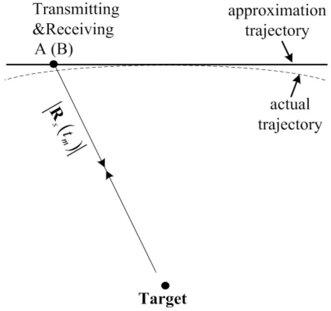
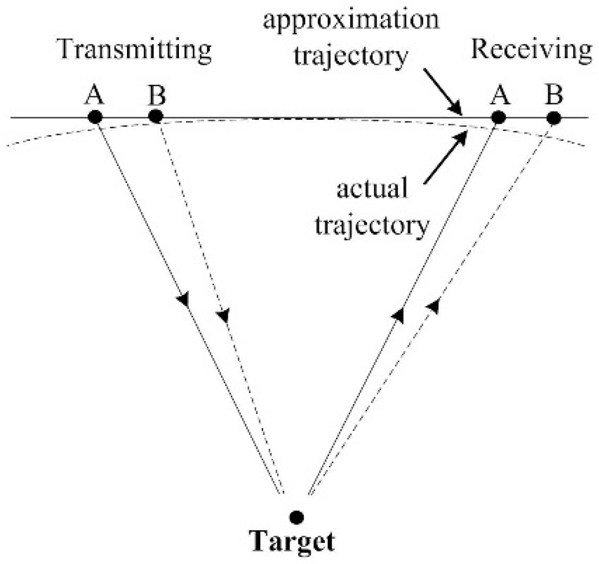
2.1. Continuous Tangent Model

Figure 1 demonstrates the actual relative motion between spaceborne SAR and the target. For convenience, time is divided into two parts: azimuth slow time $t_i$ and range fast time $\tau$. Here, $t_i=i/f_p$ ($i=0,1,2,3,\cdots$) and $f_p$ is the pulse repetition frequency (PRF). As a result, the continuous time $t$ is expressed as $t=t_i+\tau$. The mth pulse is transmitted during $\left[t_m-T/2,t_m+T/2\right]$, where $T$ denotes the pulse width. The center of the transmitting waveform is marked as A, which leaves the radar at $t_m$, reaches the target, and is reflected to the receiver at $t_n+\Delta \tau$. Similarly, another point B is transmitted at $t_m+{\tau }_s$ and received at $t_n+\Delta \tau +{\tau }_r$.

In the stop-go model, as demonstrated in Figure 2, the relative trajectory is approximated as a straight line during the aperture time. Transmitting and receiving are assumed to occur at the same position, which indicates that the two-way distances for points A and B are the same, and the width of the transmitting pulse equals the width of the echo from one isolated point.

The continuous rectilinear model was first applied to airborne FMCW SAR imaging [16], while Liu et al. applied the model to SAR imaging [15]. As demonstrated in Figure 3, the continuous rectilinear model assumes that SAR moves along a straight line without stopping. The model decomposes relative motion into two kinds. One is the relative motion between adjacent pulses, which indicates that the transmitting and corresponding receiving occur in different pulse repetition periods. The other is relative motion during one pulse, which implies that different points in the same pulse propagate along different transmitting and receiving paths, i.e., ${\tau }_r\ne {\tau }_s$.

The continuous rectilinear model does not account for the curvature of the orbit and the approximated trajectory is still a straight line [15]. As the aperture time becomes longer, this approximation will induce increasingly unacceptable errors at the edge of the synthetic aperture. The proposed continuous tangent model is demonstrated in Figure 4. It includes the advantages of the continuous rectilinear model and furthermore approximates relative trajectories during every transmitting period and every receiving period as tangential segments, respectively. The two-way distance for every sampling point can then be calculated more accurately, especially at the edge of a synthetic aperture, because this novel motion model is much closer to the actual relative motion compared with existing models.

We denote distance vectors during the mth transmitting period and the nth receiving period as $R_s(t_m,\tau )$ and $R_r(t_n,\tau )$, respectively. In the continuous tangent model, $R_s(t_m,\tau )$ and $R_r(t_n,\Delta \tau +\tau )$ can be expressed as

$$R_s\left(t_m,\tau \right)\approx R_s(t_m)+V_m\tau \tau \in \left[-\frac{T}{2},\frac{T}{2}\right]$$

(1)

$$R_r\left(t_n,\Delta \tau +\tau \right)\approx R_r(t_n,\Delta \tau )+V_r\tau \tau \in \left[\frac{T}{2}-\Delta \tau ,\frac{1}{f_p}-\Delta \tau -\frac{T}{2}\right]$$

(2)

where $V_m$ and $V_r$ are relative velocity vectors at $t_m$ and $t_n+\Delta \tau$, respectively.

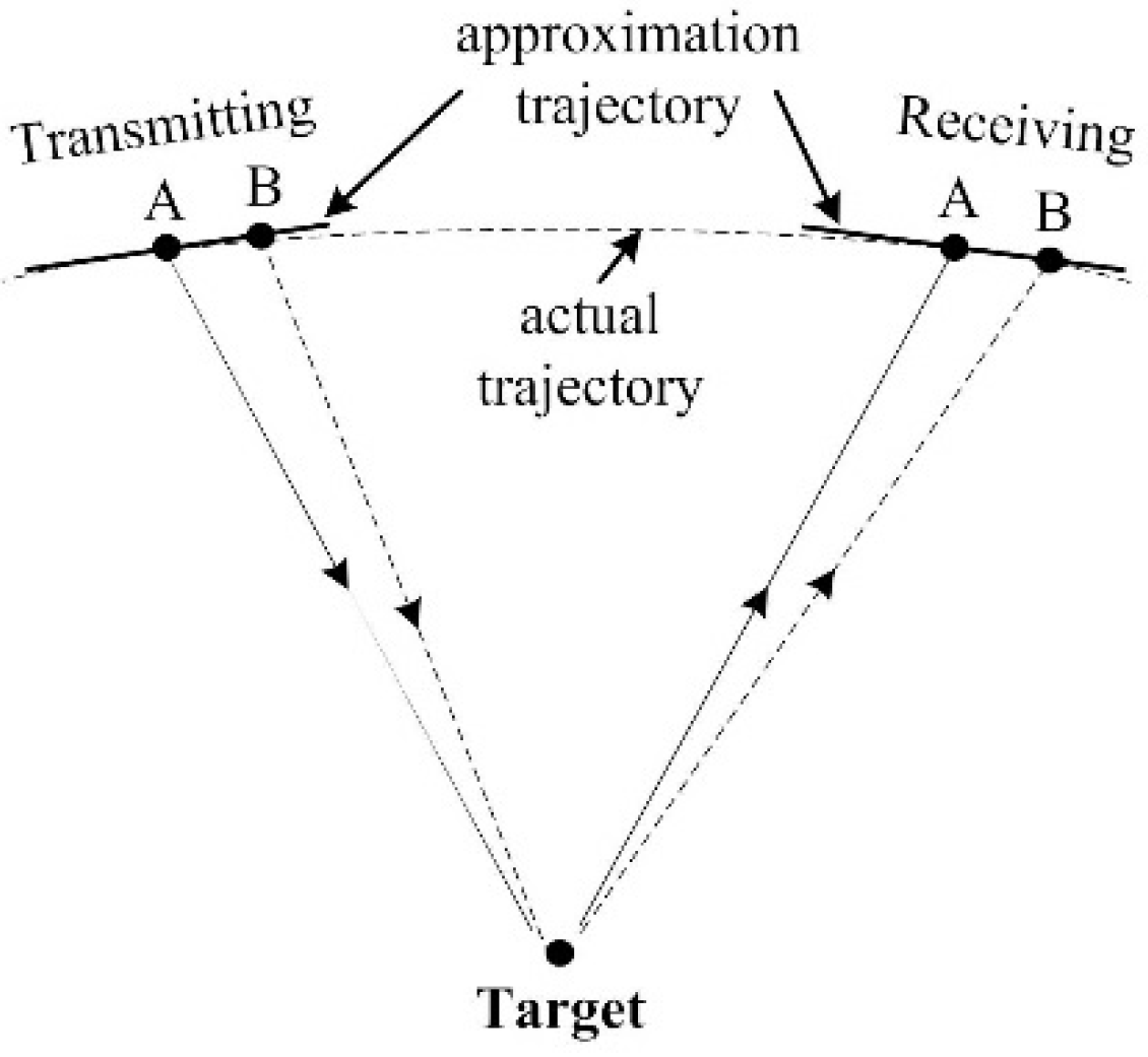
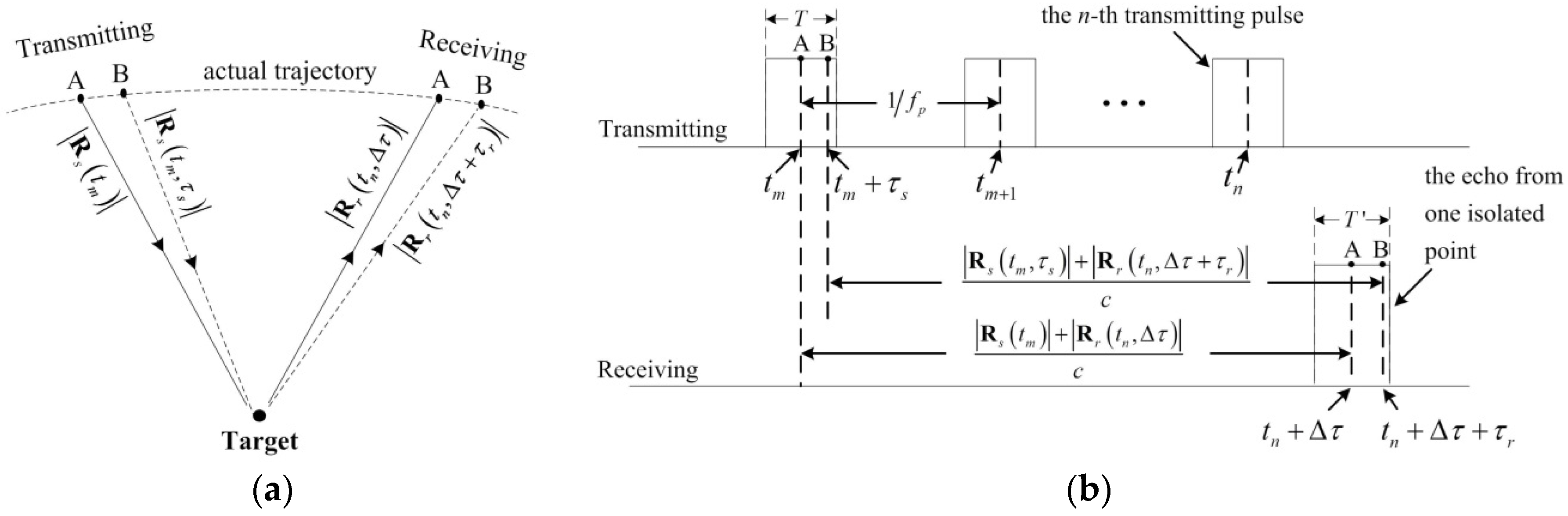
2.2. Two-Way Distance

The two-way distance for point A in Figure 4 is

$$R_A\left(t_m;t_n+\Delta \tau \right)=\left|R_s\left(t_m\right)\right|+\left|R_r\left(t_n,\Delta \tau \right)\right|=c\cdot \left[\left(n-m\right)/f_p+\Delta \tau \right]$$

(3)

where $c$ is the speed of light. The difference between $\left|R_s\left(t_m\right)\right|$ and $\left|R_r\left(t_n,\Delta \tau \right)\right|$ can be derived as (see Appendix A)

$$\left|R_r\left(t_n,\Delta \tau \right)\right|-\left|R_s\left(t_m\right)\right|=2\Delta V_m{t}_m+2\Delta r_m$$

(4)

where $\Delta V_m$ and $\Delta r_m$ are the transmitting–receiving rate and the transmitting–receiving constant, respectively. They can be expressed as

$$\Delta V_m=\frac{V_a\cdot V_m}{c}$$

(5)

$$\Delta r_m=\frac{R_s(t_0)\cdot V_m}{c}$$

(6)

where $V_a$ denotes the average relative velocity vector during the period $\left[t_0,t_{m-1}\right]$.

The two-way distance for point B is

$$\begin{array}{ll}{R}_B\left(t_m+{\tau }_s;t_n+\Delta \tau +{\tau }_r\right)& =\left|R_s\left(t_m,{\tau }_s\right)\right|+\left|R_r\left(t_n,\Delta \tau +{\tau }_r\right)\right|\\ & =R_A\left(t_m\right)+c\cdot \left[{\tau }_r-{\tau }_s\right]\\ & =2\left|R_s\left(t_m\right)\right|+2\Delta V_m{t}_m+2\Delta r_m+c\cdot \left[{\tau }_r-{\tau }_s\right]\end{array}$$

(7)

where ${\tau }_r$ and ${\tau }_s$ satisfy (see Appendix B)

$${\tau }_s=\frac{\left(c-k_1\right)}{\left(c+k_2\right)}{\tau }_r$$

(8)

and

$$k_1=V_r\cdot R_r\left(t_n,\Delta \tau \right)/\left|R_r\left(t_n,\Delta \tau \right)\right|=\left|V_r\right|\cdot \cos {\theta }_r$$

(9)

$$k_2=V_m\cdot R_s\left(t_m\right)/\left|R_s\left(t_m\right)\right|=\left|V_m\right|\cdot \cos {\theta }_s$$

(10)

where ${\theta }_r$ is the angle between $V_r$ and $R_r\left(t_n,\Delta \tau \right)$ and ${\theta }_s$ is the angle between $V_m$ and $R_s\left(t_m\right)$.

Because the time difference between transmitting and receiving is very small, $\left|V_r\right|\approx \left|V_m\right|$, ${\theta }_r\approx {\theta }_s$, and $k_1\approx k_2$. The last term in Equation (7) can then be simplified as

$$c\cdot \left[{\tau }_r-{\tau }_s\right]=m_t{\tau }_r$$

(11)

where

$$m_t=c\cdot \left(k_1+k_2\right)/\left(c+k_2\right)\approx 2\left|V_m\right|\cos {\theta }_s$$

(12)

$\left|V_m\right|$ and $\cos {\theta }_s$ vary with azimuth slow time and the looking angle. As demonstrated in Figure 5, for a fixed looking angle, $\left|V_m\right|\cos {\theta }_s$ varies linearly with the azimuth time. Therefore, $m_t$ can be approximated as:

$$m_t=2k_m{t}_m$$

(13)

where $k_m$ is the time-scaling factor.

According to Equations (7), (11) and (13), the two-way distance $R_w\left(t_n,\tau \right)$ for the point received at $t_n+\tau$ can be expressed as

$$\begin{array}{l}{R}_w\left(t_n,\tau \right)\\ =2\left|R_s\left(t_m\right)\right|+2\Delta V_m{t}_m+2\Delta r_m+2k_m{t}_m\left\{\tau +\left(n-m\right)/f_p-\left[2\left|R_s\left(t_m\right)\right|+2\Delta V_m{t}_m+2\Delta r_m\right]/c\right\}\\ \approx 2\left|R_s\left(t_m\right)\right|+2\Delta V_m{t}_m+2\Delta r_m+2k_m{t}_m\left[\widehat{\tau }-\frac{2\left|R_s\left(t_m\right)\right|}{c}\right]\end{array}$$

(14)

where $\widehat{\tau }=\tau +\left(n-m\right)/f_p$.

3. Echo Expression of Spaceborne SAR Based on the Continuous Tangent Model

The SAR echo expression is the foundation for deriving an imaging algorithm. Because the amplitude weighting is usually not taken into account in the derivation of SAR imaging algorithms [16,18], the weighting factor of the antenna pattern is ignored. The echo from an isolated point can be expressed as

$$S\left(t_i,\widehat{\tau }\right)=\sigma \cdot a\left[\widehat{\tau }-\frac{R_w\left(t_i,\widehat{\tau }\right)}{c}\right]\cdot \exp \left\{j\phi \left[\widehat{\tau }-\frac{R_w\left(t_i,\widehat{\tau }\right)}{c}\right]\right\}\cdot \exp \left[-j\frac{2\pi }{\lambda }{R}_w\left(t_i,\widehat{\tau }\right)\right]$$

(15)

where $\sigma$ is the scattering cross-section of the target, $a\left(\widehat{\tau }\right)$ is the rectangular amplitude modulation, $R_w\left(t_i,\widehat{\tau }\right)$ is the two-way distance, and $\lambda$ is the wavelength. In this paper, we use a chirp signal as the transmitting signal, i.e., $\phi \left(\widehat{\tau }\right)=-\pi b{\widehat{\tau }}^2$, where $b$ is the linear frequency modulation rate.

By substituting Equation (14) into Equation (15), SAR echo received at $t_m+\widehat{\tau }$ can be expressed as

$$\begin{array}{ll}S\left(t_m,\widehat{\tau }\right)& =\sigma \cdot a\left[\left(1-\frac{2k_m{t}_m}{c}\right)\left(\widehat{\tau }-\frac{2\left|R_s\left(t_m\right)\right|}{c}\right)-\frac{2}{c}\left(\Delta V_m{t}_m+\Delta r_m\right)\right]\\ & \cdot \exp \left\{-j\pi b{\left[\widehat{\tau }-\frac{2\left|R_s\left(t_m\right)\right|}{c}-\frac{2}{c}\left(\Delta V_m{t}_m+\Delta r_m\right)\right]}^2+j{\phi }_1\left(t_m\right)+j{\phi }_2\left({t_m}^2\right)\right\}\\ & \cdot \exp \left\{-j\frac{4\pi }{\lambda }\left[\left(1-\frac{2k_m{t}_m}{c}\right)\left|R_s\left(t_m\right)\right|+k_m\widehat{\tau }{t}_m+\Delta V_m{t}_m+\Delta r_m\right]\right\}\end{array}$$

(16)

where

$${\phi }_1\left(t_m\right)=\frac{4\pi b{k}_m{t}_m}{c^2}\cdot \left(\widehat{\tau }-\frac{2\left|R_s\left(t_m\right)\right|}{c}\right)\cdot \left[c\left(\widehat{\tau }-\frac{2\left|R_s\left(t_m\right)\right|}{c}\right)-2\Delta r_m\right]$$

(17)

$${\phi }_2\left({t_m}^2\right)=-\frac{4\pi b{k}_m{t_m}^2}{c^2}\left(\widehat{\tau }-\frac{2\left|R_s\left(t_m\right)\right|}{c}\right)\left[k_m\left(\widehat{\tau }-\frac{2\left|R_s\left(t_m\right)\right|}{c}\right)+2\Delta V_m\right]$$

(18)

According to spaceborne SAR system parameters designed for 0.2-meter resolution, ${\phi }_1\left(t_m\right)$ and ${\phi }_2\left({t_m}^2\right)$ will not exceed 1°, which hardly affects the focusing quality. Therefore, Equation (16) can be simplified as

$$\begin{array}{ll}S\left(t_m,\widehat{\tau }\right)& \approx \sigma \cdot a\left[\left(1-\frac{2k_m{t}_m}{c}\right)\left(\widehat{\tau }-\frac{2\left|R_s\left(t_m\right)\right|}{c}\right)-\frac{2}{c}\left(\Delta V_m{t}_m+\Delta r_m\right)\right]\\ & \cdot \exp \left\{-j\pi b{\left[\widehat{\tau }-\frac{2\left|R_s\left(t_m\right)\right|}{c}-\frac{2}{c}\left(\Delta V_m{t}_m+\Delta r_m\right)\right]}^2\right\}\\ & \cdot \exp \left\{-j\frac{4\pi }{\lambda }\left[\left(1-\frac{2k_m{t}_m}{c}\right)\left|R_s\left(t_m\right)\right|+k_m\widehat{\tau }{t}_m+\Delta V_m{t}_m+\Delta r_m\right]\right\}\end{array}$$

(19)

If constants are omitted, the Fourier transformation of Equation (19) along the range time can be expressed as

$$\begin{array}{ll}S\left(t_m,f_{\tau }\right)& =\exp \left[-j4\pi \left(\frac{1}{\lambda }+\frac{f_{\tau }}{c}\right)\left|R_s\left(t_m\right)\right|\right]\\ & \cdot \exp \left(j\pi \frac{{f_{\tau }}^2}{b}\right)\cdot \exp \left[j\pi \left(\frac{4k_m{t}_m{f}_{\tau }}{\lambda b}+\frac{4k_m^2{t}_m^2}{{\lambda }^{2}b}\right)\right]\\ & \cdot \exp \left[-j4\pi \left(\frac{1}{\lambda }+\frac{f_{\tau }}{c}\right)\Delta V_m{t}_m\right]\cdot \exp \left[-j4\pi \left(\frac{f_{\tau }}{c}\right)\Delta r_m\right]\end{array}$$

(20)

where $f_{\tau }$ denotes frequency in the range domain.

For comparison, echo expressions based on the stop-go model and the continuous rectilinear model are listed as Equations (21) [4] and (22) [15], respectively:

$$S_s\left(t_i,f_{\tau }\right)=\exp \left[-j4\pi \left(\frac{1}{\lambda }+\frac{f_{\tau }}{c}\right)\left|R_s\left(t_m\right)\right|\right]\cdot \exp \left(j\pi \frac{{f_{\tau }}^2}{b}\right)$$

(21)

$$\begin{array}{ll}{S}_a\left(t_i,f_{\tau }\right)& =\exp \left[-j4\pi \left(\frac{1}{\lambda }+\frac{f_{\tau }}{c}\right)\left|R_s\left(t_m\right)\right|\right]\cdot \exp \left(j\pi \frac{{f_{\tau }}^2}{b}\right)\\ & \cdot \exp \left[j\pi \left(\frac{4V^2{t}_m{f}_{\tau }}{\lambda b\left|R_s\left(t_m\right)\right|}+\frac{4V^4{t}_m^2}{{\lambda }^{2}b{\left|R_s\left(t_m\right)\right|}^2}\right)\right]\cdot \exp \left[-j\frac{4\pi V^2}{c\lambda }{t}_m\right]\end{array}$$

(22)

where $V$ denotes the flight speed.

By comparing Equations (20)–(22), differences between these three echo expressions can be summarized as follows:

(1) Relative to Equation (21), Equation (20) has three new phase terms: the third, fourth, and fifth terms. If these terms are not compensated for, they will have varying effects on focusing quality. The third phase will lead to asymmetric distortion of side lobes. The fourth phase results in the offset of the Doppler centroid and causes further offset of imaging results along the azimuth. The fifth term represents the linear variation with $f_{\tau }$, which means that an offset of the range migration is produced. Therefore, the azimuthal matching filter cannot be designed according to the right range gate, which causes azimuthal defocusing.

(2) Compared with Equation (22), Equation (20) more fully emphasizes the space-variant properties of spaceborne SAR echoes by introducing three factors: $\Delta V_m$, $\Delta r_m$ and $k_m$. These factors are different for different positions in the swath, which can be observed from Equations (5), (6), and (13). Therefore, the new echo expression, Equation (20), can describe echoes much more precisely for a wider swath. This can also be proven by the simulation results in Section 5, which demonstrate that the imaging algorithm based on Equation (20) achieves better focusing quality than that based on Equation (22) at the azimuth edge of the swath, although both algorithms have nearly the same performance at the swath center. Since $k_m$, $\Delta V_m$, and $\Delta r_m$ are important, their space-variant properties and influence on focusing quality will be analyzed in the following.

3.1. Time-Scaling Factor

Suppose $k_{m,p}$ and $k_{m,c}$ denote time-scaling factors corresponding to a certain target P_T in the swath and the swath center, respectively. When the echo from P_T is processed, $k_{m,p}$ should be adopted during imaging. If $k_{m,p}$ is replaced by $k_{m,c}$, according to Equation (20) the residual phase after compensation is

$$\Delta {\psi }_{k_m}\left(f_{\eta },f_{\tau }\right)=\left(\frac{4k_{m,p}\pi }{\lambda b}\right)\cdot \left(f_{\tau }{t}_{k,p}+\frac{k_{m,p}}{\lambda }{t_{k,p}}^2\right)-\left(\frac{4k_{m,c}\pi }{\lambda b}\right)\cdot \left(f_{\tau }{t}_{k,c}+\frac{k_{m,c}}{\lambda }{t_{k,c}}^2\right)$$

(23)

where

$$t_{k,p}\approx \frac{R_p}{V_p}\cos {\phi }_p-\frac{\lambda R_p{f}_{\eta }\sin {\phi }_p}{V_p\sqrt{4{V_p}^2-{\lambda }^2{f_{\eta }}^2}}$$

(24)

$$t_{k,c}\approx \frac{R_c}{V_c}\cos {\phi }_c-\frac{\lambda R_c{f}_{\eta }\sin {\phi }_c}{V_c\sqrt{4{V_c}^2-{\lambda }^2{f_{\eta }}^2}}$$

(25)

and $f_{\eta }$ denotes the azimuthal frequency. $V_p$, ${\phi }_p$, and $R_p$ are the equivalent velocity, the equivalent squint angle, and the reference range corresponding to P_T, respectively, and $V_c$, ${\phi }_c$, and $R_c$ are those corresponding to the swath center. The equivalent velocity $V_e$ and the equivalent squint angle ${\phi }_e$ can be calculated according to

$$V_e=\sqrt{\frac{\lambda R_0{f}_r}{2}+{\left(\frac{\lambda f_d}{2}\right)}^2}$$

(26)

$${\phi }_e=\arccos \left(-\frac{\lambda f_d}{2V_e}\right)$$

(27)

where $f_d$ is the Doppler centroid frequency, $f_r$ is the Doppler frequency rate, and $R_0$ is the reference range defined as the slant range from SAR to the target at the central moment of the aperture time.

By applying the parameters in

Table 1. Simulation parameters.

Parameters	Value
Orbital inclination	98.06°
Orbital height	680 km
Eccentricity	0.001
Elevation angle	35 °
Squint angle	±6.21 °
Beam rotation velocity	0.42 °/s
Bandwidth	1.0 GHz
Wavelength	0.03 m

, the residual phases at the swath edges are analyzed and shown in Figure 6, representing maximums of $\Delta {\psi }_{k_m}\left(f_{\eta },f_{\tau }\right)$ along range and azimuth, respectively. Figure 6a demonstrates that the residual phase is less than 0.1° at the range edge, which is 7.5 km away from the swath center. Figure 6b shows that the residual phase is less than 1° at the azimuth edge, which is also 7.5 km away from the swath center. Since both residual phases are far less than π/4 [19], the influence of the residual phases induced by the time-scaling factor on imaging performance are negligible, implying that it is not necessary to update the time-scaling factor and $k_{m,c}$ can be applied to imaging of the whole swath.

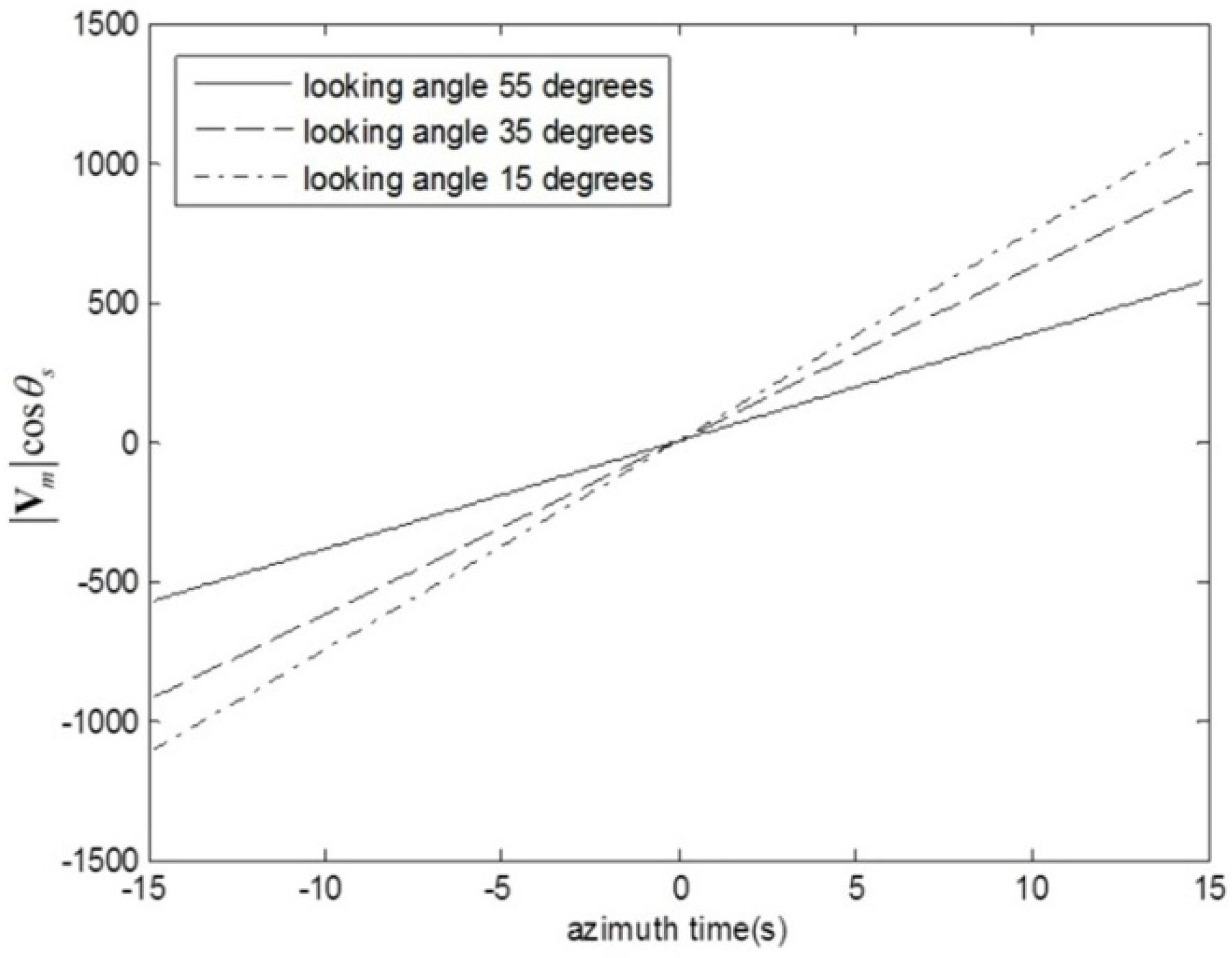
3.2. Transmitting–Receiving Rate $\Delta V_m$

If the transmitting–receiving rate $\Delta V_{m,c}$, which corresponds to the swath center, is applied to imaging for the whole swath, then the residual phase is

$$\Delta {\psi }_{\Delta V_m}\left(f_{\eta },f_{\tau }\right)=4\pi \left(\frac{1}{\lambda }+\frac{f_{\tau }}{c}\right)t_{k,p}\left(\Delta V_{m,p}-\Delta V_{m,c}\right)$$

(28)

where $\Delta V_{m,p}$ is the transmitting–receiving rate corresponding to a certain position in the swath.

According to Table 1, Figure 7 gives the residual phases $\Delta {\psi }_{\Delta V_m}\left(f_{\eta },f_{\tau }\right)$ at the range edge and the azimuth edge, respectively, which are all 7.5 km away from the swath center. As demonstrated in Figure 7a, the residual phase is less than 1.5°, which will not affect the focusing quality at the range edge. Although the residual phase in Figure 7b reaches 110° at the azimuth edge, the variation is linear with the azimuth frequency, which means only an offset along azimuth will be produced. This offset is less than 0.14 m. The above analysis indicates that the residual phase caused by applying $\Delta V_{m,c}$ instead of $\Delta V_{m,p}$ only leads to geometric distortion at the swath edge, and does not degrade the focusing quality. Therefore, $\Delta V_{m,c}$ will be adopted in imaging as the transmitting–receiving rate for the whole swath.

3.3. Transmitting–Receiving Constant $\Delta r_m$

According to Equation (6), the variation of $\Delta r_m$ in the whole swath is demonstrated in Figure 8. $\Delta r_m$ does not change along the range direction and varies linearly with the azimuth. The maximum of $\Delta r_m$ is less than two meters at the azimuth edge and the minimum is zero at the azimuth center. Therefore, according to Equation (20), an offset of the range migration will be produced by $\Delta r_m$ along the range direction and this offset varies with the azimuth.

Because of $\Delta r_m$, the azimuth matching filter designed for the range gate $R_p+\Delta r_m$ should be applied to process echoes from targets like P_T whose reference range equals $R_p$. However, if the transmitting–receiving constant corresponding to the swath center, i.e., $\Delta r_m=0$, is adopted in imaging for the whole swath, the same azimuth matching filter will be applied to process echoes for targets whose reference range equals $R_p+\Delta r_m$. This leads to a quadratic azimuthal phase error, which can be expressed as

$$\Delta {\psi }_{\Delta r_m}=\frac{\pi \lambda \Delta r_m}{8{{\rho }_a}^2{\sin }^2\phi }$$

(29)

where ${\rho }_a$ denotes the azimuthal resolution.

According to Equation (29), the phase error $\Delta {\psi }_{\Delta r_m}$ will lead to more azimuthal mismatching and defocusing as the target is much farther away from the swath center along azimuth, because $\Delta {\psi }_{\Delta r_m}$ increases with $\Delta r_m$. Therefore, different $\Delta r_m$ must be adopted for different echo segments along the azimuth.

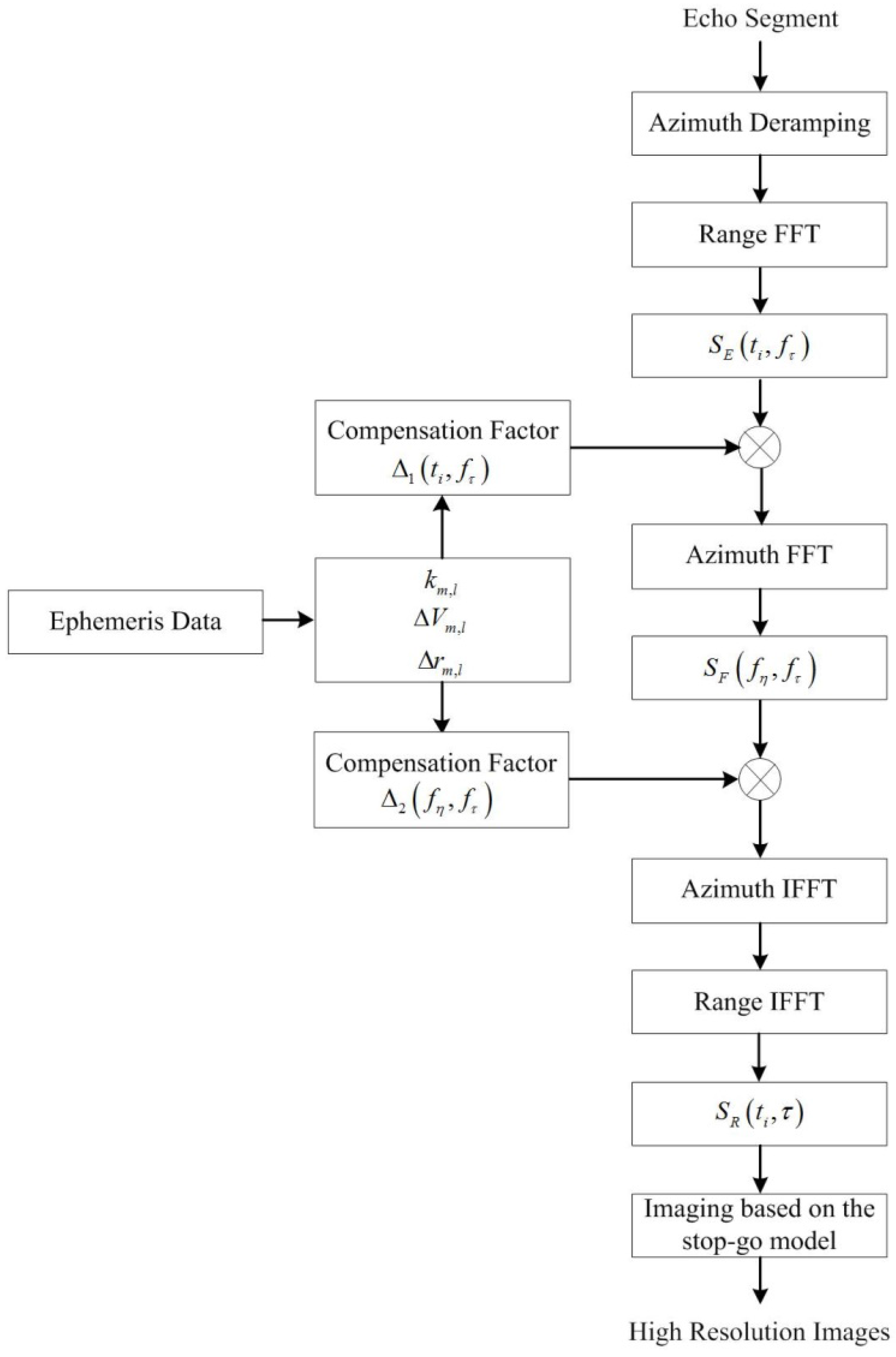
4. Imaging Compensation Algorithm

As we all know, existing spaceborne SAR imaging processors are designed based on the stop-go motion model. With the construction of the continuous tangent motion model, we have updated the SAR echo expression, and analyzed the new characteristics of the updated echo expression. In order to satisfy the existing SAR processors, we compensated the different parts between the updated echo expression and that based on the stop-go model. According to the echo expression (Equation (19)) and the space-variant analysis of three key factors, $k_m$, $\Delta V_m$, and $\Delta r_m$, a compensation algorithm with better focusing performance is proposed as follows.

(1) The first step is to divide echoes into several segments along azimuth. Every echo segment corresponds to a block of the swath. This is required because $\Delta r_m$ is space-variant and imaging for the whole swath cannot be implemented once. Otherwise, defocusing will occur at the azimuth edge of the swath, which was analyzed in Section 3.

The ephemeris data that are collected by spaceborne instruments and transmitted to the ground station with SAR echoes contain information on satellite position vectors. By applying the ephemeris data, the relative distance vectors and relative velocity vectors can be acquired. The distribution of $\Delta r_m$ across the whole swath can then be calculated according to Equation (6). It is applied to determine the segment strategy, which must guarantee that the quadratic phase error induced by $\Delta r_m$ at the edge of every swath block satisfies the requirements of the focusing quality.

For the lth echo segment, the transmitting–receiving rate $\Delta V_{m,l}$ and the transmitting–receiving constant $\Delta r_{m,l}$ corresponding to the center of the lth swath block can be calculated according to Equations (5) and (6). The time-scaling factor $k_{m,l}$ can be estimated by a linear fitting of $m_t$ according to Equation (13).

(2) The azimuthal deramping [20,21] and Fourier transform along the range are then implemented on the lth echo segment successively to acquire $S_E\left(t_i,f_{\tau }\right)$, which has the same form as Equation (20).

(3) The first compensation factor ${\Delta }_1\left(t_i,f_{\tau }\right)$ is designed as follows

$${\Delta }_1\left(t_i,f_{\tau }\right)=\exp \left[j4\pi \left(\frac{1}{\lambda }+\frac{f_{\tau }}{c}\right)\Delta V_{m,l}{t}_i\right]\cdot \exp \left[j\frac{4\pi f_{\tau }}{c}\Delta r_{m,l}\right]$$

(30)

After multiplying $S_E\left(t_i,f_{\tau }\right)$ by ${\Delta }_1\left(t_i,f_{\tau }\right)$, a Fourier transform along the azimuth is performed to acquire $S_F\left(f_{\eta },f_{\tau }\right)$, which is

$$\begin{array}{ll}{S}_F\left(f_{\eta },f_{\tau }\right)& =\exp \left(j\pi \frac{f_{\tau }^2}{b}\right)\cdot \exp \left(-j2\pi f_{\eta }\frac{R_0\cos \phi }{V}\right)\\ & \cdot \exp \left(-j\frac{4\pi \left(f_0+f_{\tau }\right)R_0\sin \phi }{c}\sqrt{1-\frac{c^2{f}_{\eta }^2}{4V^2{\left(f_0+f_{\tau }\right)}^2}}\right)\\ & \cdot \exp \{j\left(\frac{4k_{m,l}\pi }{\lambda b}\right)\cdot \left(\frac{R_0\cos \phi }{V}-\frac{\lambda R_0{f}_{\eta }\sin \phi }{V\sqrt{4V^2-{\lambda }^2{f_{\eta }}^2}}\right)\\ & \cdot \left[f_{\tau }+\frac{k_{m,l}}{\lambda }\left(\frac{R_0\cos \phi }{V}-\frac{\lambda R_0{f}_{\eta }\sin \phi }{V\sqrt{4V^2-{\lambda }^2{f_{\eta }}^2}}\right)\right]+j\frac{k_{m,l}\pi {\lambda }^2{R}_0^2}{c{V}^4{\sin }^2\phi }{f}_{\eta }^3\}\end{array}$$

(31)

(4) The second compensation factor ${\Delta }_2\left(f_{\eta },f_{\tau }\right)$ is designed as

$$\begin{array}{ll}{\Delta }_2\left(f_{\eta },f_{\tau }\right)& =\exp \{-j\left(\frac{4k_{m,l}\pi }{\lambda b}\right)\cdot \left(\frac{R_0\cos \phi }{V}-\frac{\lambda R_0{f}_{\eta }\sin \phi }{V\sqrt{4V^2-{\lambda }^2{f_{\eta }}^2}}\right)\\ & \cdot \left[f_{\tau }+\frac{k_{m,l}}{\lambda }\left(\frac{R_0\cos \phi }{V}-\frac{\lambda R_0{f}_{\eta }\sin \phi }{V\sqrt{4V^2-{\lambda }^2{f_{\eta }}^2}}\right)\right]-j\frac{k_{m,l}\pi {\lambda }^2{R}_0^2}{c{V}^4{\sin }^2\phi }{f}_{\eta }^3\}\end{array}$$

(32)

After multiplying $S_F\left(f_{\eta },f_{\tau }\right)$ with ${\Delta }_2\left(f_{\eta },f_{\tau }\right)$, an inverse Fourier transform along the azimuth equals

$$\begin{array}{ll}{S}_K\left(t_i,f_{\tau }\right)& ={\text{IFFT}}_{f_{\eta }}\left[S_F\left(f_{\eta },f_{\tau }\right)\cdot {\Delta }_2\left(f_{\eta },f_{\tau }\right)\right]\\ & =\exp \left[-j4\pi \left(\frac{1}{\lambda }+\frac{f_{\tau }}{c}\right)\left|R_s\left(t_i\right)\right|\right]\cdot \exp \left(j\pi \frac{{f_{\tau }}^2}{b}\right)\end{array}$$

(33)

(5) $S_K\left(t_i,f_{\tau }\right)$ has the same form as Equation (21), which is the echo expression based on the stop-go model. Therefore, sliding spotlight imaging algorithms based on the stop-go model can be applied to process $S_K\left(t_i,f_{\tau }\right)$ and achieve a high-resolution image for the lth echo segment. Here, the deramping ωk algorithm is adopted [13,18].

Figure 9 shows the compensation flow for every echo segment. After each echo segment has been imaged, results are stitched together along the azimuth to form a final complete image of the whole swath.

5. Simulation and Validation

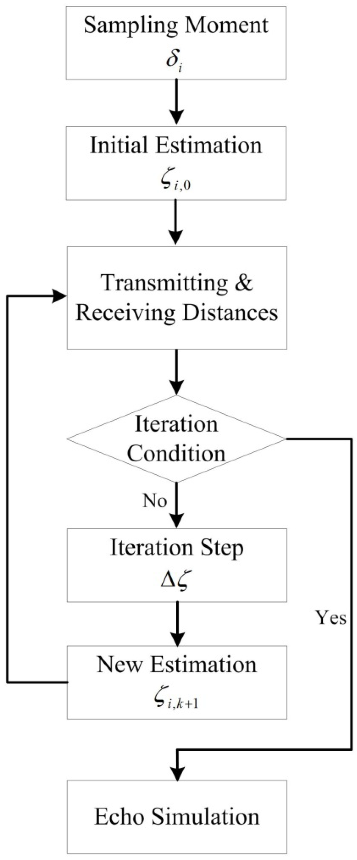
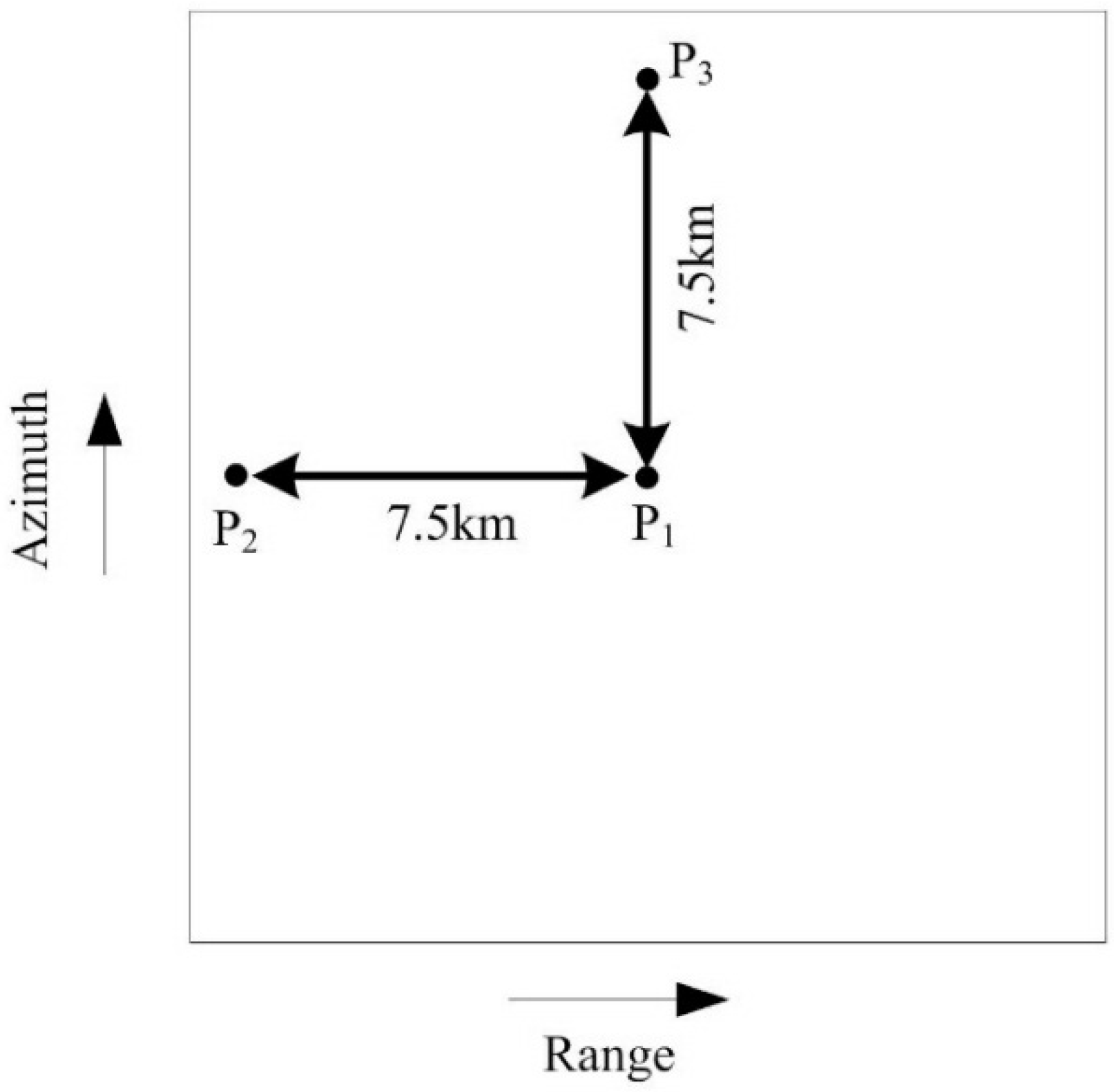
5.1. Simulation Method and Parameters

SAR echo simulation methods are typically based on the stop-go model. A new method is proposed here to simulate the continuous motion of the satellite. The key to this method is to acquire an accurate transmitting distance according to the receiving distance for every echo sampling point.

As demonstrated in Figure 1, the receiving moment ${\delta }_i$ for the ith sampling point during $\left[t_n,t_n+1/f_p\right]$ can be expressed as

$${\delta }_i=t_n+{\tau }_g+\frac{i}{F_s}i=0,1,2,\cdots$$

(34)

where ${\tau }_g$ is the sampling start time and $F_s$ is the sampling rate.

In order to calculate the transmitting moment corresponding to ${\delta }_i$, iterations are performed as demonstrated in Figure 10. Detailed steps are as follows.

(1) The initial estimation of the transmitting moment corresponding to ${\delta }_i$ is assumed to be

$${\zeta }_{i,0}={\delta }_i-2R\left({\delta }_i\right)/c$$

(35)

where $R\left({\delta }_i\right)$ is the relative distance between SAR and the target at the moment ${\delta }_i$.

(2) If Equation (36) can be satisfied, the transmitting distance is considered to be $R\left({\zeta }_{i,k}\right)$, which denotes the relative distance at ${\zeta }_{i,k}$ ($k=0,1,2,\cdots$). Otherwise, Step (3) is performed.

$$\left|\frac{R\left({\zeta }_{i,k}\right)+R\left({\delta }_i\right)}{c}-\left({\delta }_i-{\zeta }_{i,k}\right)\right|<{10}^{-15}$$

(36)

(3) Let ${\zeta }_{i,k+1}={\zeta }_{i,k}-\Delta \zeta$. $\Delta \zeta$ is

$$\Delta \zeta =\frac{\left(R\left({\zeta }_{i,k}\right)+R\left({\delta }_i\right)\right)/c-\left({\delta }_i-{\zeta }_{i,k}\right)}{2}$$

(37)

(4) Let $k=k+1$, and return to Step (2).

By performing the iteration method for every sampling point, the transmitting and receiving distances can be precisely calculated and substituted into Equation (15) to form the simulated echoes.

Simulation parameters are listed in

Table 2. Simulation parameters.

Parameters	Value
Orbital inclination	98.06°
Orbital height	680 km
Eccentricity	0.001
Elevation angle	35°
Wavelength	0.03 m
Beam width (Azimuth)	0.305°
Squint angle	±6.21°
Beam rotation velocity	0.42°/s
Signal bandwidth	1.0 GHz
Pulse width	40 μs
Pulse repetition frequency	4000 Hz

. The simulated swath covering an area of 15 km × 15 km is demonstrated in Figure 11, where three point targets, P₁, P₂, and P₃, are arranged at the center, the range edge, and the azimuth edge, respectively.

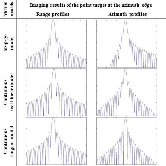
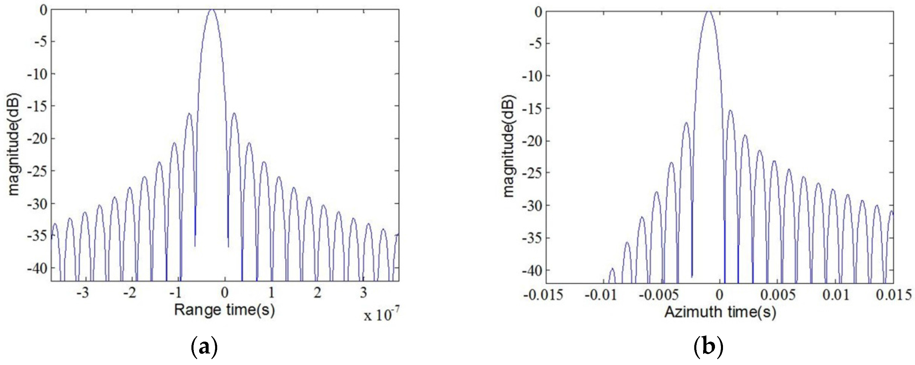
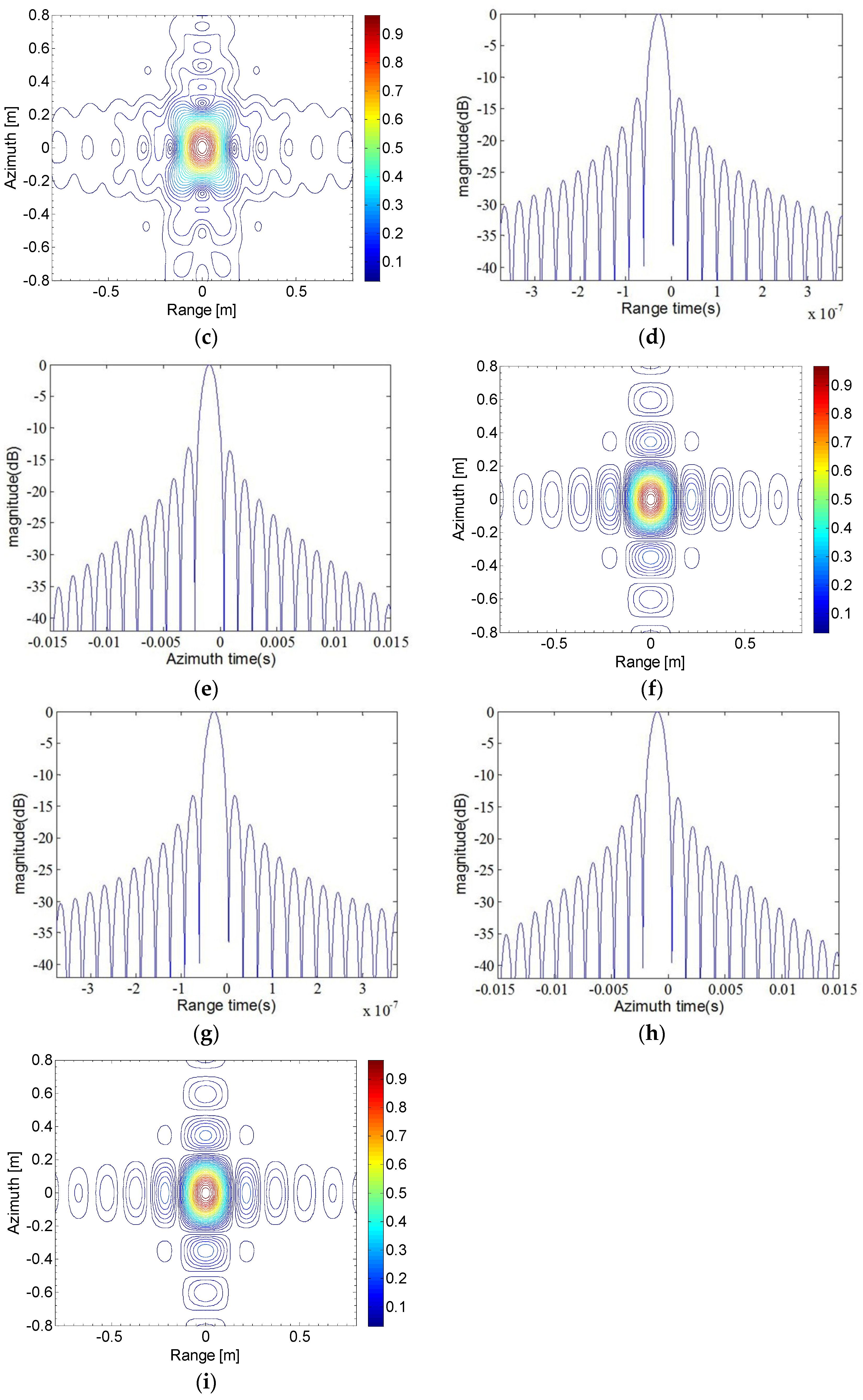
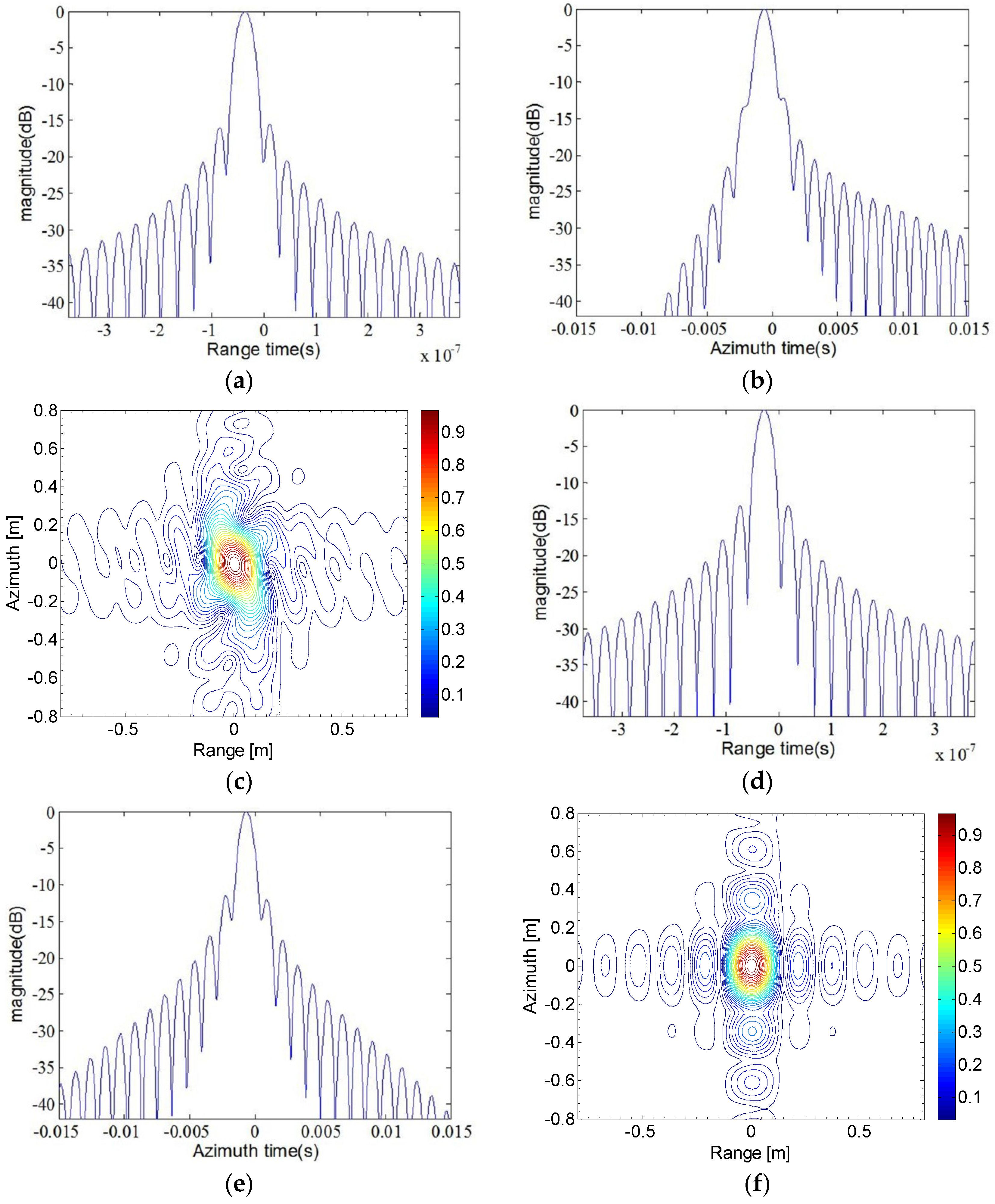
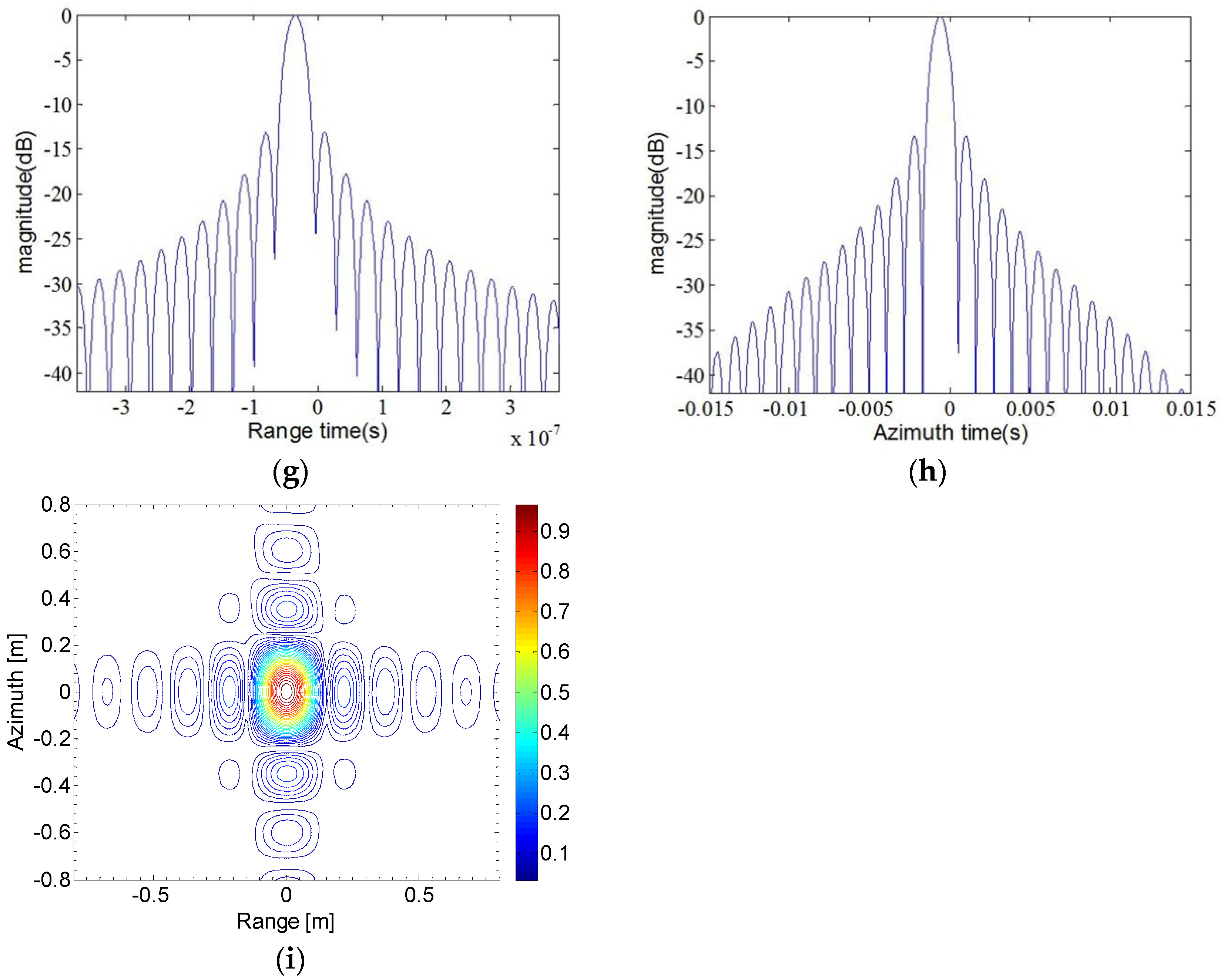
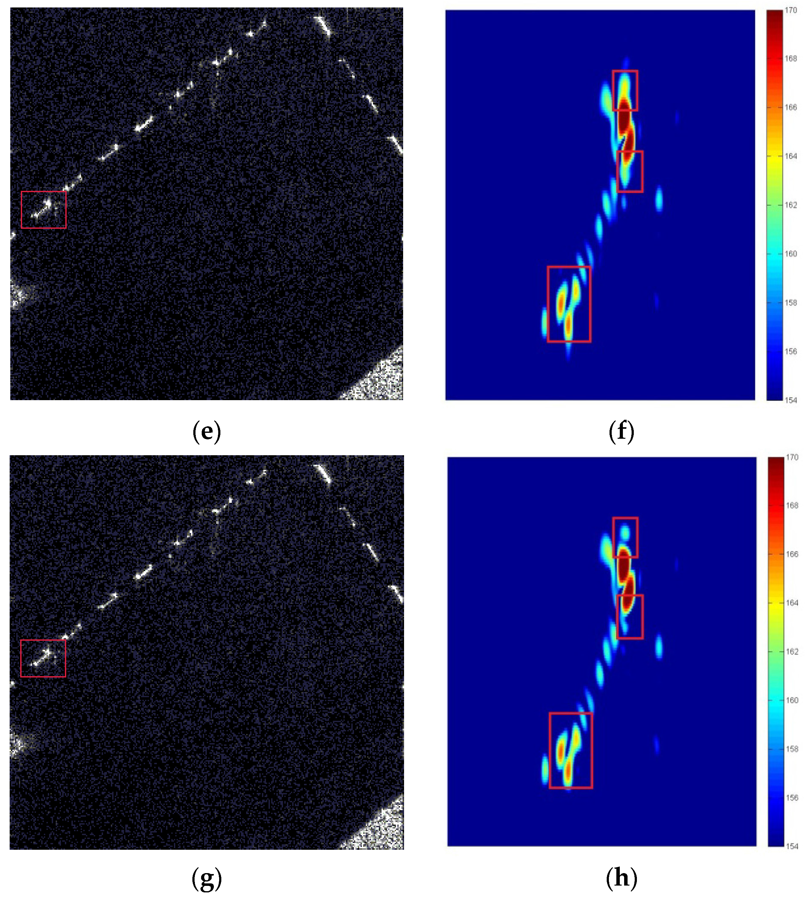
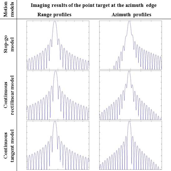
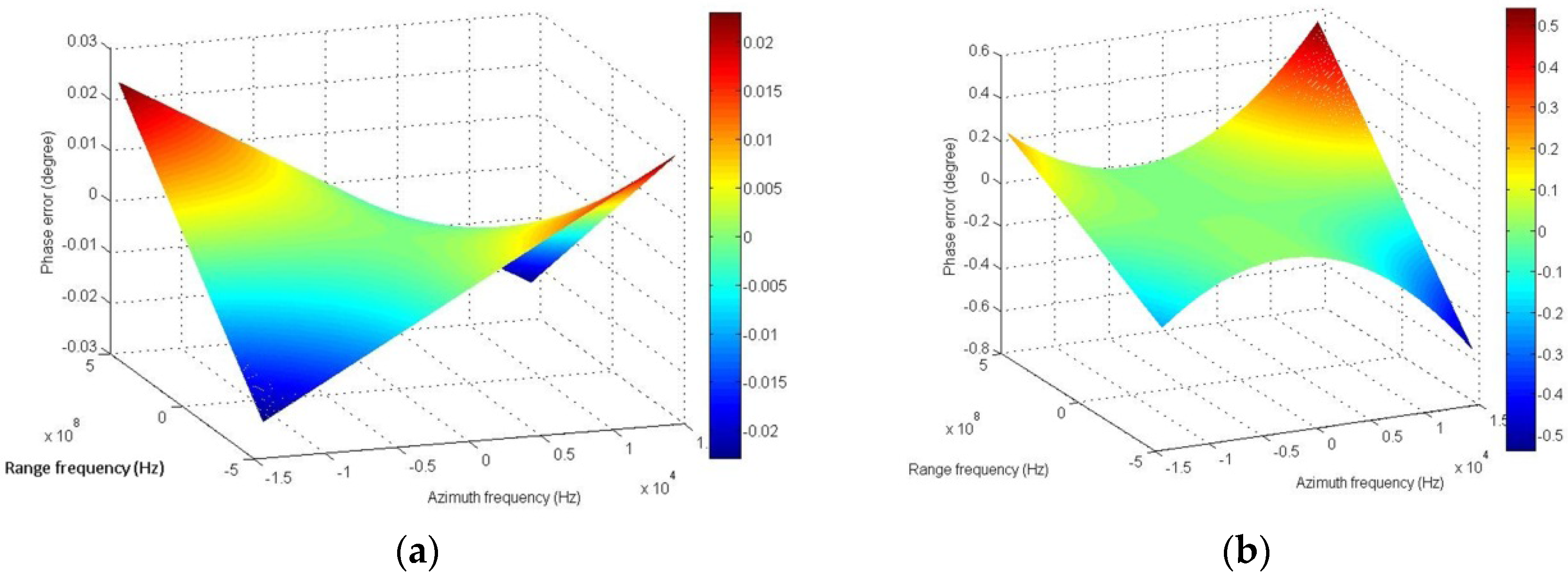
5.2. Simulation Results

Figure 12, Figure 13 and Figure 14 demonstrate the imaging results of P₁, P₂, and P₃, where the profiles represent the focusing quality along the range and azimuth, and contour maps denote the two-dimensional focusing quality. In every figure, there are three kinds of results. The first result is achieved using the Deramping ωk algorithm, which is based on the stop-go model [18]. The second is achieved according to the algorithm presented in [15], which is based on the continuous rectilinear model. The third is achieved using the novel imaging compensation method presented in this paper.

By applying resolution, peak to side lobe ratio (PSLR), and integrated side lobe ratio (ISLR) as indicators to evaluate Figure 12, Figure 13 and Figure 14, the evaluation results along the range and azimuth are presented in

Table 3. Evaluation of imaging quality along range.

Motion Model	Target	Resolution (m)	PSLR (dB)	ISLR (dB)
Stop-go model	P1	0.1444	−16.49	−13.54
	P2	0.1433	−16.10	−13.10
	P3	0.1444	−15.42	−12.51
Continuous rectilinear model	P1	0.1342	−13.25	−9.96
	P2	0.1342	−13.26	−9.96
	P3	0.1342	−13.05	−9.77
Continuous tangent model	P1	0.1342	−13.25	−9.96
	P2	0.1342	−13.25	−9.95
	P3	0.1342	−13.13	−9.80

and

Table 4. Evaluation of imaging quality along azimuth.

Motion Model	Target	Resolution (m)	PSLR (dB)	ISLR (dB)
Stop-go model	P1	0.2333	−15.64	−13.35
	P2	0.2350	−15.29	−13.05
	P3	0.2420	−11.98	−9.79
Continuous rectilinear model	P1	0.2156	−13.07	−10.39
	P2	0.2203	−13.11	−10.40
	P3	0.2250	−11.53	−8.63
Continuous tangent model	P1	0.2156	−13.08	−10.39
	P2	0.2203	−13.11	−10.41
	P3	0.2170	−13.32	−10.41

, respectively.

According to imaging profiles and evaluation results, the first imaging algorithm, which is based on the stop-go model, exhibits the worst performance. Along the range and azimuth, the main lobe corresponding to every target is broadened, which reduces the resolution. Although PSLR and ISLR are better for this method than the other two methods, it comes at the cost of a loss in resolution. Furthermore, this method brings asymmetric phenomena to azimuth side lobes, which indicates that quadratic and high-order phase errors are not compensated for completely in imaging.

The second algorithm, which is based on the continuous rectilinear model, can achieve thinner main lobes. Compared with the first method, the range resolutions are improved by about 6.35%–7.06%. The azimuth resolutions are improved by about 6.26%–7.59%. However, for P₃, which is at the azimuth edge of the swath, the azimuth resolution, PSLR, and ISLR decay obviously compared with the swath center, as demonstrated in Figure 14 and Table 4.

The algorithm based on the continuous tangent model preserves the focusing performance with the second method at the swath center and the range edge, and further improves the focusing quality at the azimuth edge. The azimuth resolution, PSLR, and ISLR corresponding to P₃ are improved by 3.56%, 1.79 dB, and 1.78 dB, respectively. As a result, focusing qualities for P₁, P₂, and P₃ are nearly the same, which indicate that imaging coherency for the whole swath is good.

To further demonstrate the performance of the proposed algorithm, a two-dimensional example is provided based on an airborne SAR image (Courtesy of Sandia National Laboratories, Airborne ISR). The resolution and size of this image are 0.1 m and 66 m × 66 m, respectively. It is deployed at the top left corner of the simulated swath, and the simulated echo can be achieved. By applying algorithms based on the stop-go model, the continuous rectilinear model, and the continuous tangent model, different imaging results are acquired (Figure 15).

There are three red rectangles in every enlarged view of the selectable portion. As shown in the bottom rectangle of Figure 15b, there are three scattering centers. However, only two centers are recognized in Figure 15d, while three centers can be distinguished in both Figure 15f,h. This indicates that the algorithm based on the stop-go model has the worst focusing quality. In the top rectangle of Figure 15b, only the edge of one scattering center exists. However, something more, caused by side lobes, appears at the same positions of Figure 15f,h. This is an isolate spot in the top rectangle of Figure 15h. The spot in the top rectangle of Figure 15f is connected with the scattering center because the algorithm based on the continuous rectilinear model has worse PSLR and ISLR than the proposed algorithm based on the continuous tangent model. The difference between middle rectangles in Figure 15f,h also demonstrates this point. As a result, the algorithm proposed in this paper has better focusing performance than other two algorithms.

5.3. Computational Load

Computational load is a key element restricting the application of an algorithm. As demonstrated in Figure 9, after the first and second compensations, echoes can be successfully focused using current algorithms based on the stop-go model. Therefore, the analysis of computational load focuses on the first and second compensations. Although the chirp scaling algorithm (CSA) [8,9] cannot achieve 0.21 m resolution and 15 km swath width for spaceborne SAR, it is worth comparing CSA and these compensations from the aspect of the computational load because CSA is recognized as an efficient algorithm and has been widely applied.

Computational load is evaluated according to the complex multiplication and addition in the algorithm. Multiplication of two complex numbers and addition of two real numbers require 6 FLOPs (floating point operations) and 1 FLOP, respectively. An FFT or IFFT of length N requires $5N{\log }_2\left(N\right)$ FLOPs [4]. Suppose sampling numbers along the azimuth and range are $N_{azi}$ and $N_{rng}$, respectively. The computational loads of CSA, and the first and second compensations in the proposed algorithm, are, respectively,

$$\begin{array}{l}{N}_{CSA}=10N_{rng}{N}_{azi}{\log }_2\left(N_{azi}\right)+10N_{rng}{N}_{azi}{\log }_2\left(N_{rng}\right)+18N_{rng}{N}_{azi}\\ N_{PA}=15N_{rng}{N}_{azi}{\log }_2\left(N_{azi}\right)+10N_{rng}{N}_{azi}{\log }_2\left(N_{rng}\right)+24N_{rng}{N}_{azi}\end{array}$$

(38)

In order to achieve 0.21 m resolution and a swath of 15 km × 15 km, $N_{azi}$ and $N_{rng}$ should be at least 118,650 and 150,000, respectively. According to Equation (38), the computational load of the first and second compensations is 1.25 times that of CSA, which indicates that the compensations are efficient.

6. Conclusions

This paper developed a continuous tangent model to describe the relative motion between a spaceborne SAR and its targets. An imaging compensation algorithm was proposed based on the new motion model. Compared with the algorithm based on the stop-go model, the novel algorithm improved the range resolutions and the azimuth resolutions by about 6.35%–7.06% and 6.26%–10.33%, respectively. Compared with the algorithm based on the continuous rectilinear model, the novel algorithm further improved the azimuth resolution, PSLR, and ISLR at the azimuth edge by 3.56%, 1.79 dB, and 1.78 dB, respectively. Simulation results indicated that the presented algorithm provided a superior and more consistent focusing quality across the whole swath.

The novel algorithm is also applicable to the updating of existing spaceborne SAR imaging processors that are designed based on the stop-go model. A pre-processing module is the only addition necessary to implement the first and second compensations, as demonstrated in Figure 9. After being processed by this pre-processing module, echoes can be successfully focused using existing processors to produce high-quality image products. The input parameters for the new algorithm are the same as the existing algorithms, which indicates that it is not necessary to change the input interface in the updating.

However, as the resolution is improved, a higher requirement for the accuracy of the motion model will be put forward. Therefore, under the condition of better resolution, the continuous tangent model should be further verified as well as the corresponding imaging compensation algorithm.

References

1. Sadjadi, F. New comparative experiments in range migration mitigation methods using polarimetric inverse synthetic aperture radar signatures of small boats. In Proceedings of the 2014 IEEE Radar Conference, Cincinnati, OH, USA, 19–23 May 2014; pp. 613–616.
2. Sadjadi, F.A. New Experiments in Inverse synthetic aperture radar image exploitation for maritime surveillance. In Proceedings of the SPIE Defense+ Security, 2014 International Society for Optics and Photonics, Baltimore, MD, USA, 5–9 May 2014; pp. 909009:1–909009:09.
3. Wang, W.Q.; Jiang, D. Integrated wireless sensor systems via near-space and satellite platforms: A review. IEEE Sens. J. 2014, 14, 3903–3914. [Google Scholar] [CrossRef]
4. Cumming, I.G.; Wong, F.H. Digital Processing of Synthetic Aperture Radar Data: Algorithms and Implementation; Artech House: Norwood, MA, USA, 2005. [Google Scholar]
5. Curlander, J.; McDonough, R. Synthetic Aperture Radar: Systems and Signal Processing; John Wiley & Sons: New York, NY, USA, 1991. [Google Scholar]
6. Lim, B.G.; Woo, J.C.; Lee, H.Y.; Kim, Y.S. A Modified subpulse SAR processing procedure based on the range-doppler algorithm for synthetic wideband waveforms. Sensors 2008, 8, 8224–8236. [Google Scholar] [CrossRef]
7. Bamler, R.; Breit, H.; Steinbrecher, U.; Just, D. Algorithms for X-SAR processing. In Proceedings of the International Geoscience and Remote Sensing Symposium, Tokyo, Japan, 18–21 August 1993; pp. 1589–1592.
8. Wang, W.Q.; Shao, H. Azimuth-variant signal processing in high-altitude platform passive SAR with spaceborne/airborne transmitter. Remote Sens. 2013, 5, 1292–1310. [Google Scholar] [CrossRef]
9. Davidson, G.W.; Cumming, I.; Ito, M.R. A chirp scaling approach for processing squint mode SAR data. IEEE Trans. Aerosp. Electron. Syst. 1996, 32, 121–133. [Google Scholar] [CrossRef]
10. Janoth, J.; Gantert, S.; Schrage, T.; Kaptein, A. From TerraSAR-X towards TerraSAR next generation. In Proceedings of the 10th European Conference on Synthetic Aperture Radar, Berlin, Germany, 3–5 June 2014; pp. 1–4.
11. Novak, L.M.; Benitz, G.R.; Owirka, G.J.; Bessette, L.A. ATR performance using enhanced resolution SAR, aerospace/defense sensing and controls. In Proceedings of the International Society for Optics and Photonics, Orlando, FL, USA, 10 June 1996; pp. 332–337.
12. Novak, L.M.; Owirka, G.J.; Netishen, C.M. Performance of a high-resolution polarimetric SAR automatic target recognition system. Lincoln Lab. J. 1993, 6, 11–24. [Google Scholar]
13. Prats-Iraola, P.; Scheiber, R.; Rodriguez-Cassola, M.; Mittermayer, J.; Wollstadt, S.; De Zan, F.; Brautigam, B.; Schwerdt, M.; Reigber, A.; Moreira, A. On the processing of very high resolution spaceborne SAR data. IEEE Trans. Geosci. Remote Sen. 2014, 52, 6003–6016. [Google Scholar] [CrossRef]
14. Mittermayer, J.; Wollstadt, S.; Prats-Iraola, P.; Scheiber, R. The TerraSAR-X staring spotlight mode concept. IEEE Trans. Geosci. Remote Sen. 2014, 52, 3695–3706. [Google Scholar] [CrossRef]
15. Liu, Y.; Xing, M.; Sun, G.; Lv, X.; Bao, Z.; Hong, W.; Wu, Y. Echo model analyses and imaging algorithm for high-resolution SAR on high-speed platform. IEEE Trans. Geosci. Remote Sens. 2012, 50, 933–950. [Google Scholar] [CrossRef]
16. Meta, A.; Hoogeboom, P.; Ligthart, L.P. Signal processing for FMCW SAR. IEEE Trans. Geosci. Remote Sens. 2007, 45, 3519–3532. [Google Scholar] [CrossRef]
17. Ribalta, A. Time-domain reconstruction algorithms for FMCW-SAR. IEEE Geosci. Remote Sens. Lett. 2011, 8, 396–400. [Google Scholar] [CrossRef]
18. Teng, L.; Wu, J.; Huang, Y.; Yang, J. A deramping based Omega-k algorithm for wide scene spotlight SAR. In Proceedings of the International Conference on Systems and Informatics, Yantai, China, 18–20 May 2012; pp. 2089–2092.
19. Carrara, W.G.; Goodman, R.S.; Majewski, R.M. Spotlight Synthetic Aperture Radar: Signal Processing Algorithms; Artech House: Norwood, MA, USA, 1995. [Google Scholar]
20. Mittermayer, J.; Moreira, A.; Loffeld, O. Spotlight SAR data processing using the frequency scaling algorithm. IEEE Trans. Geosci. Remote Sens. 1999, 37, 2198–2214. [Google Scholar] [CrossRef]
21. Wang, G.D. A deramp chirp scaling algorithm for processing spaceborne spotlight SAR data. In Proceedings of the ICMMT 4th International Conference on Microwave and Millimeter Wave Technology, Beijing, China, 18–21 August 2004; pp. 659–663.
Figure 1. (a) The actual relative motion between spaceborne Synthetic Aperture Radar (SAR) and the target; (b) The corresponding time sequence of transmitting and receiving.
Remotesensing 08 00223 g001
Figure 2. The stop-go model.
Remotesensing 08 00223 g002
Figure 3. The continuous rectilinear model.
Remotesensing 08 00223 g003
Figure 4. The continuous tangent model.
Remotesensing 08 00223 g004
Figure 5. Variation of | V m | cos θ s with the azimuth time and the looking angle by applying parameters in Table 1. Three lines are presented under looking angles 15, 35 and 55 degrees, which represent the low, medium and high looking angles, respectively. For a looking angle, | V m | cos θ s varies linearly with the azimuth time.
Remotesensing 08 00223 g005
Figure 6. Phase errors induced by the time-scaling factor k m . The distribution of the residual phases in the two-dimensional frequency domain at the range edge (a) and the azimuth edge (b).
Remotesensing 08 00223 g006
Figure 7. Phase errors induced by the transmitting–receiving rate Δ V m . The distribution of the residual phases in the two-dimensional frequency domain at the range edge (a) and the azimuth edge (b).
Remotesensing 08 00223 g007
Figure 8. The variation of Δ r m in the whole swath. It is obvious that Δ r m does not change along the range direction, and varies linearly with the azimuth. The absolute maximum of Δ r m is less than two meters at the azimuth edge, and the minimum is zero at the swath center.
Remotesensing 08 00223 g008
Figure 9. An imaging compensation algorithm based on the continuous tangent model.
Remotesensing 08 00223 g009
Figure 10. A workflow diagram of the simulation method. The core of the flow chart is to accurately estimate the transmitting moment corresponding to every sampling moment within the synthetic aperture time. Afterwards, the transmitting and receiving distances can be calculated and substituted into the echo expression to achieve simulated echoes.
Remotesensing 08 00223 g010
Figure 11. The simulated swath: P1 is at the swath center. P2 and P3 are at the range edge and the azimuth edge, respectively, which are all 7.5 km away from P1.
Remotesensing 08 00223 g011
Figure 12. Imaging results of P1, the point at the swath center. (ac) The range profile, the azimuth profile and the contour map achieved using the Deramping ωk algorithm based on the stop-go model; (df) The range profile, the azimuth profile and the contour map achieved using the algorithm based on the continuous rectilinear model; (gi) The range profile, the azimuth profile and the contour map achieved using the novel imaging compensation method presented in this paper.
Remotesensing 08 00223 g012aRemotesensing 08 00223 g012b
Figure 13. Imaging results of P2, the point at the range edge. Images (ai) are in accordance with Figure 12.
Remotesensing 08 00223 g013aRemotesensing 08 00223 g013b
Figure 14. Imaging results of P3, the point at the azimuth edge. Images (ai) are in accordance with Figure 12.
Remotesensing 08 00223 g014aRemotesensing 08 00223 g014b
Figure 15. Comparison of imaging results: (a) the real SAR image; (b) enlarged view of selectable portion in (a); (c) stop-go model image; (d) enlarged view of selectable portion in (c); (e) the continuous rectilinear model image; (f) enlarged view of selectable portion in (e); (g) continuous tangent model image; (h) enlarged view of selectable portion in (g).
Remotesensing 08 00223 g015aRemotesensing 08 00223 g015b