Forest Disturbances and Regrowth Assessment Using ALOS PALSAR Data from 2007 to 2010 in Vietnam, Cambodia and Lao PDR

Abstract

This paper aims to develop a new methodology for monitoring forest disturbances and regrowth using ALOS PALSAR data in tropical regions. In the study, forest disturbances and regrowth were assessed between 2007 and 2010 in Vietnam, Cambodia and Lao People’s Democratic Republic. The deforestation rate in Vietnam has been among the highest in the tropics in the last few decades, and those in Cambodia and Lao are increasing rapidly. L-band ALOS PALSAR mosaic data were used for the detection of forest disturbances and regrowth, because L-band SAR intensities are sensitive to forest aboveground biomass loss. The methodology used here combines SAR data processing, which is particularly suited for change detection, forest detection and forest disturbances and regrowth detection using expectation maximization, which is closely related to fuzzy logic. A reliable training and testing database has been derived using AVNIR-2 and Google Earth images for calibration and validation. Efforts were made to apply masking areas that are likely to show different SAR backscatter temporal behaviors from the forests considered in the study, including mangroves, inundated forests, post-flooding or irrigated croplands and water bodies, as well as sloping areas and urban areas. The resulting forest disturbances and regrowth map (25-m resolution) indicates disturbance rates of −1.07% in Vietnam, −1.22% in Cambodia and −0.94% in Lao between 2007 and 2010, with corresponding aboveground biomass losses of 60.7 $Tg$, 59.2 $Tg$ and 83.8 $Tg$, respectively. It is expected that the method, relying on free of charge data (ALOS and ALOS2 mosaics), can be applied widely in the tropics.

1. Introduction

Forests act as a carbon source through deforestation and degradation [1] and as a carbon sink through forest regrowth [2]. However, major uncertainties exist in the estimates of the carbon emissions that result from forest disturbances and in the uptake of carbon through forest regrowth. At present, forest destruction is a major source of carbon emissions and a primary factor in the loss of biodiversity [3]. In the tropics, deforestation is considered to contribute approximately 15% of man-made global emissions [4], though the rate of tropical deforestation has been reported to have decreased from 0.16 Mkm${}^2$·y${}^{-1}$ in the 1990s to 0.13 Mkm${}^2$·y${}^{-1}$ in the first decade of the 21st century [5]. Estimates of tropical forest area and change still contain considerable uncertainty, impeding the estimation of the carbon emissions caused by deforestation and forest degradation in the tropics [1]. The call to reduce uncertainties in estimating changes in tropical forest cover is also driven by the reporting needs outlined in the Reducing Emissions from Deforestation and forest Degradation (REDD+) program.

Remote sensing offers considerable potential for supporting forest monitoring, because it provides long-term and repetitive observation over large areas. The main remote sensing data source is optical sensors, with Landsat data being the most frequently-used dataset for mapping forest cover and its changes. Among the most cited studies, the Landsat-based detection of Trends in Disturbance and Recovery (LandTrendr) approach allows the spectral trajectories of land surface changes to be extracted from yearly Landsat time series stacks [6]. A companion interpretation approach needed for the expert interpretation of the image stacks themselves and, thus, the derivation of reference data has been developed and integrated in a software package known as TimeSync [7]. A new algorithm for continuous change detection and classification (CCDC) based on all available Landsat data was recently developed by [8]. In addition, Landsat data have been used to map global forest loss and gain from 2000 to 2012 (and yearly updated since 2012) at a spatial resolution of 30 m [9]. In this study, 654,178 Landsat 7 Enhanced Thematic Mapper Plus (ETM+) scenes were analyzed to create a set of cloud-free image observations; this process required the use of one million central processing unit-core hours on 10,000 computers. In tropical regions, infrequent cloud-free data and the fast recovery of vegetation can hamper the detection of changes in forest cover. Some studies have also raised doubts regarding the validity of Hansen’s map [10,11].

Synthetic aperture radar (SAR) is one of the most promising remote sensing methods for the mapping of forest disturbances. SAR enables imaging in all weather conditions at any time of day or night, and long-wavelength radar data are sensitive to forest aboveground biomass (AGB) [12,13,14] at HH [15,16] and HV polarizations [17,18,19,20]. However, SAR data are rarely used for mapping forest disturbances, because SAR data are not systematically available and because the forest and carbon community is more familiar with optical data. Note that Shimada et al. [21] recently used Advanced Land Observing Satellite (ALOS) Phased Array type L-band Synthetic Aperture Radar (PALSAR) and ALOS2 PALSAR2 mosaics to produce global maps (25-m resolution) of forest and non-forest cover (2007 to 2010), from which some maps of forest losses and gain were generated based on thresholds. However, these maps are not currently available.

The goal of this paper is to assess forest disturbances and regrowth in tropical regions between 2007 and 2010 using 25-m resolution ALOS PALSAR data. The targeted area is Southeast Asia, specifically Vietnam, Cambodia and Lao People’s Democratic Republic (PDR). This area plays an important role in environmental protection and biodiversity and is of interest with regard to its socio-economy and the living conditions of forest-dependent populations. Thus, Southeast Asia’s tropical forests are of importance in the context of the global carbon balance. The deforestation rate in Southeast Asia has been among the highest in the tropics [22]. In its global Forest Resources Assessment (FRA) in 2010, the United Nations Food and Agriculture Organisation (FAO) reported a net annual forest area loss in Southeast Asia of 2.4 Mha in the 1990s, with values of 0.4 Mha and 1.0 Mha for 2000 to 2005 and 2005 to 2010, respectively [5], resulting in a forest area loss of 29.5 Mha between 1990 and 2010. Stibig et al. [23] estimated a drop in Southeast Asia’s total forest cover from approximately 268 Mha in 1990 to 236 Mha in 2010, resulting in a forest area loss of 32 Mha between 1990 and 2010. In 20 years, a forested area comparable to the size of Vietnam, or approximately 6.5% of the region’s total land area, disappeared. The dominant patterns of forest change relate to forest conversion, logging, the replacement of natural forests by forest plantations, shifting cultivation, new infrastructures and burning. Vietnam is among the countries with the greatest annual changes in primary forest area and planted forest area in the last 20 years. According to the FAO, the extent of primary forest in Vietnam decreased at rates of 6.94%, 15.6% and 1.21% in 1990 to 2000, 2000 to 2005 and 2005 to 2010, respectively, whereas the extent of planted trees increased at rates of 7.8%, 6.4% and 4.7% in the same periods. The FAO currently considers Vietnam to be a reforesting country because tree plantations are included as forests in the FRA process. Monoculture plantations cover extensive areas of Southeast Asia, with dominant species including oil palm, rubber, wattles and coconut. Forest plantations are interesting because they are believed to increase the carbon sequestered from the atmosphere and to mitigate future climate change, although forest plantations achieve 28% less carbon storage than natural forest [24]. To reduce greenhouse gas emissions, extending the rotation length in forest management was highlighted in Article 3.4 of the Kyoto Protocol as a way to help countries meet their commitments [25]. However, there is a general trend towards decreasing the rotation length to optimize yields. Note that in Southeast Asia, large Vietnamese companies have recently leased vast tracts of land for plantations in Lao PDR and Cambodia, with disastrous consequences for local communities and the environment. By the end of 2012, 2.6 Mha of land in Cambodia had been leased (1.2 Mha for rubber), and at least 1.1 Mha has been given to land concessionaires in Lao PDR through a process marked by a lack of consultation and forced evictions [26].

In this paper, we assess forest disturbances and regrowth using a new semi-automated method. The method is adapted for large-scale forest disturbance monitoring using free of charge ALOS or ALOS2 mosaic data for tropical regions where the deforestation rate is still high. This method combines SAR data processing, which is particularly suited for change detection from SAR, masks areas that may induce misdetection or false alarms (such as inundated crops/forests and high terrain slopes) and expectation maximization (EM). EM is very closely related to fuzzy classification approaches and has the advantage of requiring no binary decisions regarding class memberships. EM has been successfully applied to SAR data, but mainly over small test areas [27,28,29]. In this study, PALSAR’s 25-m spatial resolution is preserved by using a multi-image speckle filter, which is crucial for the detection of small change areas, followed by the masking of areas that may show temporal SAR backscatter behaviors that could be incorrectly attributed to disturbed forest or regrowth.

Section 2 provides information on the study region and data. Section 3 describes the approach used for forest disturbance and regrowth detection, and Section 4 discusses the results.

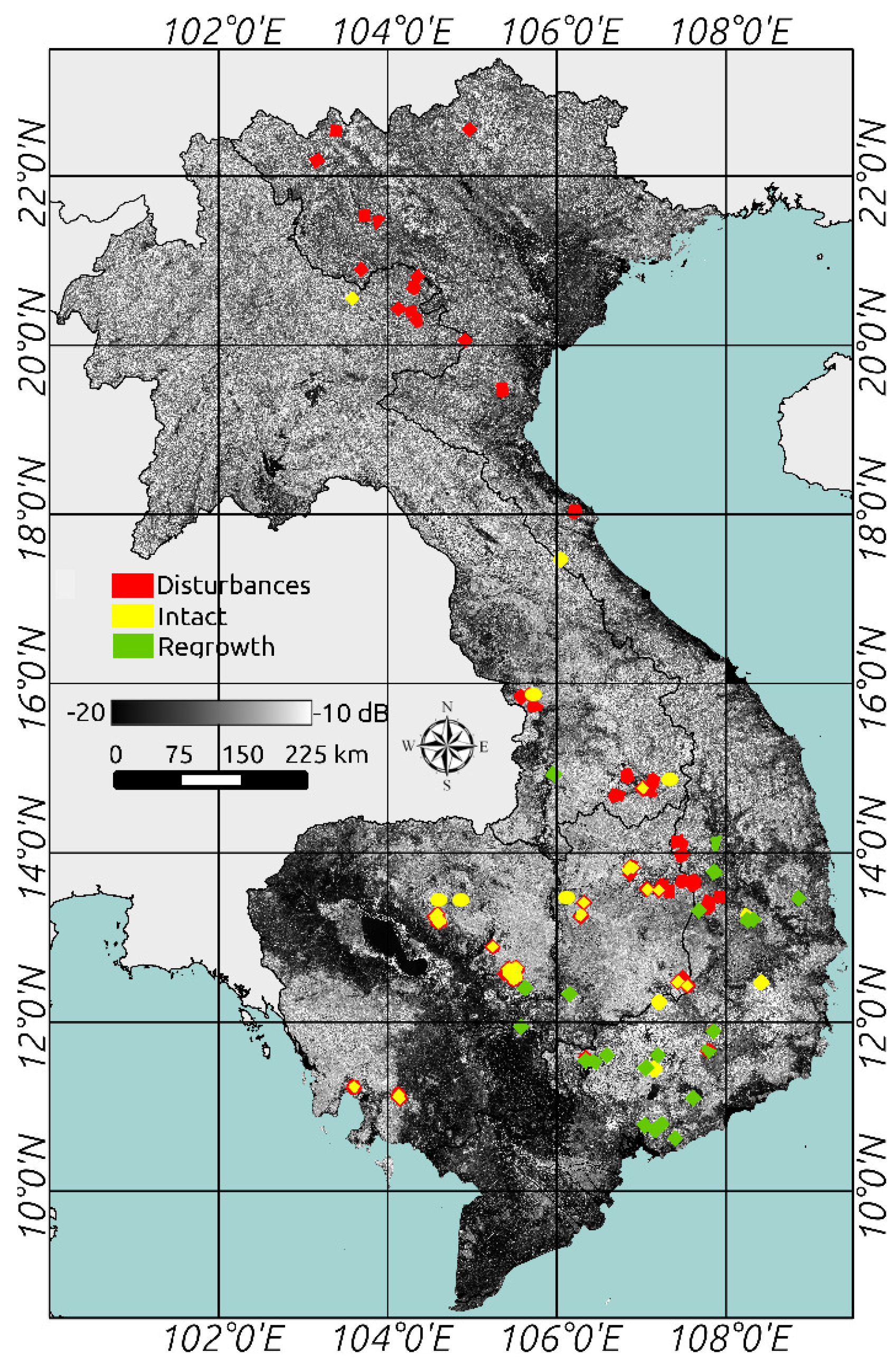
2. Study Sites and Data

2.1. Study Sites

The study area includes Vietnam, Cambodia and Lao PDR, which are located in Continental Southeast Asia, from ∼9 to 24${}^{\circ }$N and from ∼100 to 110${}^{\circ }$E. Most of Southeast Asia is warm to hot year round, and the climate is dominated by the annual monsoon cycle, with its alternating wet and dry seasons.

Vietnam is located between ∼9 and 23${}^{\circ }$N and covers a total area of more than 332,000 km${}^2$. This country has a single rainy season during the south monsoon (from May to September) with abundant rainfall, which annually exceeds 1000 mm in nearly every region. The annual rainfall is even higher in the hills, especially those facing the sea, and ranges from 2000 to 2500 mm. The country is mountainous in the northwest and in the central highlands facing the South China Sea, with peaks reaching up to 2450 m. In the north near Hanoi and in the south near Ho Chi Minh City, there are extensive low-lying regions in the Red River delta and the Mekong delta, respectively. Cambodia is located ∼10–13${}^{\circ }$N of the equator, and its surface area exceeds 181,000 km${}^2$. The mean daily temperature rises and falls in the summer and winter months, respectively, but does not correspond exactly to the wet and dry seasons, effectively creating four annual seasons in this country. Lao PDR is a landlocked country located from ∼20 to 26${}^{\circ }$N and from ∼100 to 107${}^{\circ }$E. This country covers a total area of approximately 237,000 km${}^2$, three quarters of which are mountains and plateaus, which are mostly in the north. Lao PDR enjoys a tropical climate with two distinct seasons; the rainy season lasts from the beginning of May to the end of September, and the dry season spans October to April.

2.2. Remote Sensing Data

Five hundred four ALOS PALSAR mosaic tiles with 25-m resolution over all of Vietnam, Cambodia and Lao PDR were supplied by the Japan Aerospace Exploration Agency (JAXA). Mosaic data were available yearly from 2007 to 2010 and are spatially square (approximately $112\times 112$ km or 1${}^{\circ }$ of latitude and 1${}^{\circ }$ of longitude). The signal was converted into γ${}^{\circ }$ values using the following equation:

$${\gamma }^o=10.lo{g}_{10}\left(D{N}^2\right)+CF$$

(1)

where γ${}^{\circ }$ is the normalised backscatter divided by the cosine of the local incidence angle, $DN$ is the digital number and $CF$ is the calibration factor described in [30].

Digital elevation models (DEMs) from the Shuttle Radar Topography Mission (SRTM) were used to derive terrain slopes. In addition, high- to very high-resolution (VHR) optical data were used to derive a spatially-explicit training and testing database (refer to Section 2.3 below) to calibrate the method and assess forest disturbances and regrowth. To this end, we used 33 ALOS Level 1.5 geocoded Advanced Visible and Near Infrared Radiometer 2 (AVNIR-2) (10-m resolution), processed by JAXA, and VHR Google Earth images [31]. As introduced by Dorais and Cardille [32], Google Earth images are actually a relatively untapped new source of validation data for remote sensing studies. These images are captured at a wide variety of dates, are mostly cloud free and have sufficient resolution to very easily distinguish many types of land covers and land uses, including forest disturbances.

2.3. The Training and Testing Database

We extracted several polygons of natural forests and disturbed and regrowth areas in test sites through visual interpretation of the AVNIR-2 and Google Earth images. The disturbance polygons were drawn in reference to at least two AVNIR-2 images acquired close in time to two PALSAR observation dates. Only clear-cut areas were extracted as disturbance polygons. Selective logging was not considered because the 25-m resolution is not sufficient to detect such small disturbances. The forest regrowth polygons were drawn in the same way and were mostly located in tree plantations. To assess false positives, natural forest areas that were very unlikely to have undergone human-induced disturbances, such as parts of protected national parks located far from villages, roads and rivers, were analyzed. The numbers and sizes of the reference polygons are shown in

Table 1. Numbers and sizes of the reference polygons constituting the training and testing database for forest disturbances and regrowth assessment.

	No. of Areas	Mean Size (ha)	Surface (ha)
No Disturbances	59	209.1	12,333
Disturbances	86	5.3	428
Regrowth	23	2.7	144

, and their spatial distribution is shown in Figure 1. Note that the number of polygons and the surface areas related to forest disturbances and regrowth polygons, e.g., 428 and 144 ha, respectively, are very small compared to the surface area of the whole study site (75 Mha).

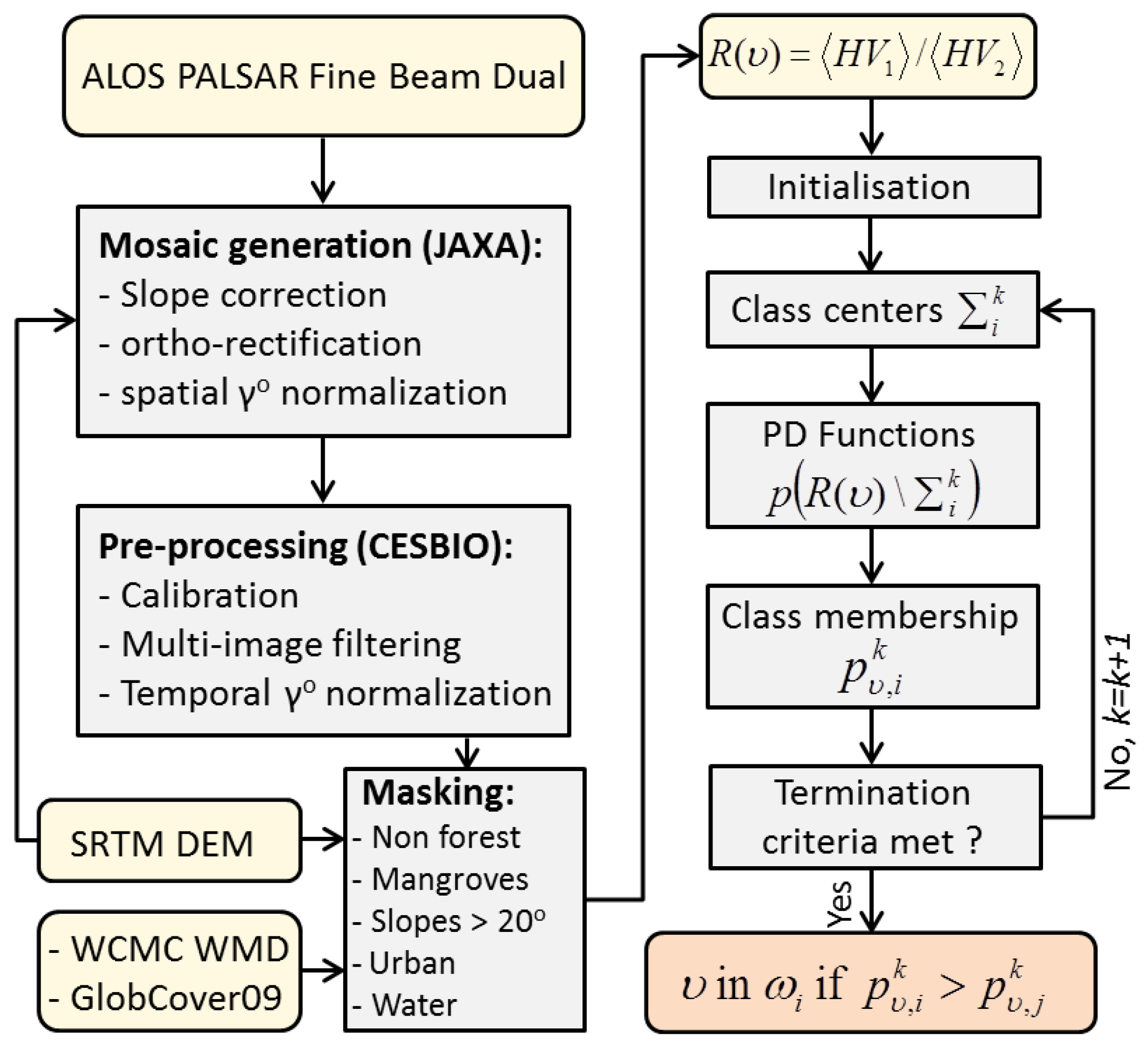
3. Forest Disturbances and Regrowth Detection Method

3.1. ALOS PALSAR Mosaic Generation and Pre-Processing

The goal of a change-detection algorithm is to detect significant changes while rejecting unimportant ones. Preprocessing steps, including, for example, geometric and intensity adjustments, are used to filter out common types of unimportant changes before making the change-detection decision [33]. Initially, the 504 ALOS images used in this study were processed by JAXA using the large-scale mosaicking algorithm described in [34]. This algorithm includes ortho-rectification, slope correction and radiometric calibration between neighboring strips. The resulting images were perfectly overlaid, and the equivalent number of looks (ENL) of ALOS PALSAR data was 16. However, the presence of speckle noise can induce a high number of false alarms in the change-detection procedure. A filter was therefore applied to decrease the speckle effect while preserving the spatial resolution and the fine structure present in the image; this strategy is particularly suited for change detection. The method used [35,36] provides images with reduced speckle effects from multi-temporal and multi-polarized images (four dates at HH and HV polarizations in our case). It is based on the following relation:

$$J_k\left(\mathit{\nu }\right)=\frac{\langle I_k\left(\mathit{\nu }\right)\rangle }{N}\sum _{i=1}^N\frac{I_i\left(\mathit{\nu }\right)}{\langle I_i\left(\mathit{\nu }\right)\rangle }\text{with}k=1,...,N$$

(2)

where $J_k\left(\mathit{\nu }\right)$ is the radar intensity of the output image k at pixel position ν, $I_i\left(\mathit{\nu }\right)$ is the radar intensity of the input image i, $\langle I_i\left(\mathit{\nu }\right)\rangle$ is the local average intensity of the input image i, $\langle I_k\left(\mathit{\nu }\right)\rangle$ is the local average intensity of the input image k and N is the number of images. The resulting ENL is 112, with associated standard deviation of the backscatter ${\gamma }^o$ caused by speckle noise of approximately 0.4 dB. The 504 images were then geolocated (latitude/longitude coordinates were assigned to each pixel) using the coordinates of the four image corners and mosaicked.

Considering the multi-temporal data, environmental sources of noise mainly consist of soil and vegetation moisture. All of the images were acquired during the same (rainy) season, thereby minimizing temporal changes caused by these environmental effects. However, the rainy season is not the most appropriate season for forest disturbances and regrowth assessment because the γ${}^{\circ }$ differences between forest and disturbed areas decrease as the accumulated precipitation increases, as highlighted by Motohka et al. [37]. However, the backscatter contrast over forest and bare soil remains sufficient for our purpose, even during the rainy season, as will be shown in Section 4.1. To further minimize temporal changes caused by environmental conditions or the SAR radiometric stability, the multi-temporal intensity data were normalized to have approximately the same temporal mean and variance over the ‘forest pixels’ using the methodology of Du et al. [38]. In this method, pixels at the same location in two different scenes form corresponding pixel pairs. A selection of dense forest pixel pairs was performed, avoiding the obviously changed (i.e., deforested) ones. Pixels were selected by applying principal component analysis over the forest pixels (see Section 4.2 for details about the selection of the forest pixels). Only pixels with low absolute values on the second principal component axis were chosen to ensure that the first principal component axis would show strong and significant Pearson correlation coefficients, i.e., greater than 0.9. When only two scenes acquired at two different times were involved (for example, scene year 2010 as the master and 2009 as the slave), under a linear relationship assumption, the formula for the radiometric transform of scene year 2009 should be:

$$\begin{array}{cc}\hfill \widetilde{{\gamma }_{09}}\left(\mathit{\nu }\right)=& {\gamma }_{09}\left(\mathit{\nu }\right).{\mathcal{G}}_{09}+{\mathcal{O}}_{09}\hfill \\ \hfill =& {\gamma }_{09}\left(\mathit{\nu }\right).\frac{{\sigma }_{10}}{{\sigma }_{09}}+{\mu }_{10}-\frac{{\sigma }_{10}}{{\sigma }_{09}}.{\mu }_{09}\hfill \end{array}$$

(3)

where ${\mathcal{G}}_{09}$ is the gain associated with scene year 2009, ${\mathcal{O}}_{09}$ is the offset associated with scene year 2009, ${\gamma }_{09}\left(\mathit{\nu }\right)$ is the uncorrected intensity of scene year 2009 at pixel position ν and $\widetilde{{\gamma }_{09}}\left(\mathit{\nu }\right)$ is the corrected signal value for scene year 2009. The means and standard deviations for the two scenes are $({\mu }_{10},{\mu }_{09})$ and $({\sigma }_{10},{\sigma }_{09})$, respectively. Because we aimed to assess forest disturbances from 2007 to 2010, considering the data from 2010 as a reference reveals:

$$\begin{array}{cc}& {\mathcal{G}}_{10}=1\hfill \\ & {\mathcal{O}}_{10}=0\hfill \\ & {\mathcal{G}}_{09}=\frac{{\sigma }_{10}}{{\sigma }_{09}}\hfill \\ & {\mathcal{O}}_{09}={\mu }_{10}-\frac{{\sigma }_{10}}{{\sigma }_{09}}.{\mu }_{09}\hfill \\ & {\mathcal{G}}_{08}=\frac{\widetilde{{\sigma }_{09}}}{{\sigma }_{08}}=\frac{{\sigma }_{09}}{{\sigma }_{08}}.{\mathcal{G}}_{09}.{\mathcal{G}}_{10}\hfill \\ & {\mathcal{O}}_{08}=\widetilde{{\mu }_{09}}-\frac{\widetilde{{\sigma }_{09}}}{{\sigma }_{08}}.{\mu }_{08}={\mu }_{09}-\frac{{\sigma }_{09}}{{\sigma }_{08}}.{\mu }_{08}.{\mathcal{G}}_{09}.{\mathcal{G}}_{10}+{\mathcal{O}}_{09}\hfill \\ & {\mathcal{G}}_{07}=\frac{\widetilde{{\sigma }_{08}}}{{\sigma }_{07}}=\frac{{\sigma }_{08}}{{\sigma }_{07}}.{\mathcal{G}}_{08}.{\mathcal{G}}_{09}.{\mathcal{G}}_{10}\hfill \\ & {\mathcal{O}}_{07}=\widetilde{{\mu }_{08}}-\frac{\widetilde{{\sigma }_{08}}}{{\sigma }_{07}}.{\mu }_{07}={\mu }_{08}-\frac{{\sigma }_{08}}{{\sigma }_{07}}.{\mu }_{07}.{\mathcal{G}}_{08}.{\mathcal{G}}_{09}.{\mathcal{G}}_{10}+{\mathcal{O}}_{08}\hfill \end{array}$$

(4)

All intensity images were corrected using the gains and offsets from Equations (4) and used below.

3.2. Masking Undesirable Areas

L-band SAR backscatter at both HH and HV polarizations is sensitive to forest AGB, but HV-polarized backscatter is less sensitive to environmental sources of noise. Therefore, we first extracted forest pixels by applying a threshold to ${\gamma }_{HV}$. Mangroves have characteristic forest-floor changes caused by tidal shifts and may show different temporal SAR backscatter behaviors than the forests considered in this study. Because the present study did not check the applicability of the method to mangroves, mangroves were masked using the World Conservation Monitoring Centre (WCMC) world map of mangrove distribution (WMD) [39]. Similarly, significant temporal backscatter variations at both HV and HH polarizations have been observed over flooded forests because of changing water elevations. Therefore, we masked land areas subject to inundations using data from the Digital Chart of the World [40]. Topographical heterogeneities are a major source of uncertainties in radar backscattering. Thus, we discarded pixels with a terrain slope exceeding 20${}^{\circ }$. To assess the possible underestimation of forest disturbances resulting from the slope masking process, we estimated the neglected forest surface area over slopes exceeding 20${}^{\circ }$. To this end, we used the Landsat Vegetation Continuous Fields tree cover layers (VCF) [41] that contain estimates of the percentage of horizontal ground in each 30-m pixel covered by woody vegetation greater than 5 m in height. We degraded the VCF resolution by averaging the pixels to the resolution of the terrain slope, e.g., 90 m, and considered VCF pixels as forest if their value was ≥ 50%. We found that forests over slopes exceeding 20${}^{\circ }$ represent 5.3% of the whole study area and 11.3% of total forest area. We assume that the underestimation of forest disturbances is much smaller than 11.3%, assuming that most human-induced changes do not occur over such steep slopes (although natural disturbances may occur). Some crops, such as rice, may also exhibit significant temporal backscatter variations depending on whether they are inundated, newly sowed or fully developed. Post-flooding or irrigated (or aquatic) croplands were masked using the GlobCover 2009 land cover map [42], as were urban areas and water bodies.

3.3. Forest Disturbances and Regrowth Detection Indicators

The classical change-detection approach in SAR remote sensing involves using the ratio of the local means in the neighborhood of each pair of colocated pixels because of the multiplicative nature of speckle. This approach assumes that a change in the scene will appear as a modification of the local mean value of the image. This detection method is robust to speckle noise, but it is limited to the comparison of first-order statistics. Bujor et al. [43] studied higher-order statistics for change detection in SAR images and concluded that the ratio of means was useful for step changes and that the second-and third-order log-cumulants were useful for progressive changes appearing in consecutive images in multi-temporal series. Because we aimed to detect larges changes at one-year temporal frequency in this study (three years for forest regrowth), we assumed that a modification of the local mean value is sufficiently reliable to detect changes. An analysis window is required for the computation of the local mean value estimation used here. An inappropriate window size can produce mis- and over-detections, and small analysis window sizes are required to yield high-resolution change maps. The key problem is how to choose the largest window size that robustly detects the changes while being small enough to preserve the resolution of the final map without creating misdetections [44].

The choice of the polarization (or combination of polarizations) to be used is controversial. Some studies have used HV-polarized L-band data [37,45,46] or a combination of HH- and HV-polarized data to detect forest changes [3]. PALSAR multi-temporal ${\gamma }_{HV}$ and ${\gamma }_{HH}$ for intact forest, deforested and reforested areas calculated using the database described in Section 2.3 are shown in Figure 2. The numbers of samples used in the analysis for each class were 6144, 6848 and 2304, respectively. A part of the intact forest database is used in this analysis to ensure comparable statistics computed for each class.

To assess the potential of each polarization for forest disturbances and regrowth detection, we used receiver operating characteristic (ROC) curves. In fact, trade-offs between detections and false alarms can be assessed by plotting the probability of true positive detection, $P_{td}$, against the probability of false positive alarm, $P_{fa}$. For a given threshold, $P_{td}$ is defined as the fraction of the deforested or reforested area for which the change measure exceeds the threshold, whereas $P_{fa}$ is the equivalent fraction for undisturbed forest. The ROC curves based on our training and testing database (Section 2.3) and derived separately for the ratios of ${\gamma }_{HV}$, ${\gamma }_{HH}$, ${\gamma }_{HV}$/${\gamma }_{HH}$ and E(${\gamma }_{HV}$,${\gamma }_{HH}$), where E is the average value, are shown in Figure 3. Each point on the ROC curves corresponds to a particular threshold. For forest disturbance detection (left, Figure 3), the four indicators exhibit significant differences, e.g., for $P_{fa}$ = 10%, the $P_{td}$ values for ${\gamma }_{HV}$, ${\gamma }_{HH}$, ${\gamma }_{HV}$/${\gamma }_{HH}$ and E(${\gamma }_{HV}$,${\gamma }_{HH}$) are 98%, 75%, 54% and 89%, respectively. For forest regrowth detection (right, Figure 3), for $P_{fa}$ = 10%, the detection probabilities for the four indicators are 97%, 86%, 38% and 92%, respectively. The ratio of ${\gamma }_{HV}$ showed the best results for the detection of both forest disturbances and regrowth. Therefore, we decided to use the time series ratios in ${\gamma }_{HV}$ for this study.

In the following, we assumed gamma-distributed multilook SAR intensities. Local statistics can deviate from the Gamma distribution in the presence of texture, but in our case of forest or bare soil, the texture can be considered as negligible at about a 25-m resolution. The probability density function of the intensity ratio R between two images $H{V}_1$ and $H{V}_1$ $R\left(\mathit{\nu }\right)=\langle H{V}_1\left(\mathit{\nu }\right)\rangle |\langle H{V}_2\left(\mathit{\nu }\right)\rangle$ of a homogeneous region is found to depend only on the ratio of average intensities $\langle H{V}_1\rangle |\langle H{V}_2\rangle$ and not directly on the average intensities $\langle H{V}_1\rangle$ and $\langle H{V}_2\rangle$:

$$p(R\left(\mathit{\nu }\right)\setminus {\Sigma }_i)=\frac{{\displaystyle R{\left(\mathit{\nu }\right)}^{N-1}\prod _{k=1}^N(2N-k)}}{(N-1)!{\Sigma }_i^N.{(1+\frac{R\left(\mathit{\nu }\right)}{{\Sigma }_i})}^{2N}}$$

(5)

where ${\Sigma }_i$ is the class ${\omega }_i$ mean ratio. A significance test can be performed on the ratio image to assign an unknown pixel to the class ${\omega }_i$:

$$R\left(\mathit{\nu }\right)\in {\omega }_i\text{if}\frac{p(R\left(\mathit{\nu }\right)\setminus {\Sigma }_i)}{p(R\left(\mathit{\nu }\right)\setminus {\Sigma }_j)}>\tau \forall j\ne i$$

(6)

where τ is a threshold, assuming that a priori probabilities of occurrence of the classes are unknown, e.g., uniformly distributed. Given a set of three classes (intact natural forest, disturbances and regrowth, corresponding to $i=[1,2,3]$), each ratio can be assigned to one of these classes by considering the normalized probability of class membership:

$$R\left(\mathit{\nu }\right)\in {\omega }_i=\frac{p(R\left(\mathit{\nu }\right)\setminus {\Sigma }_i)}{\sum _{j=1}^{3}p(R\left(\mathit{\nu }\right)\setminus {\Sigma }_j)}$$

(7)

The most obvious approach is to threshold the ratio image. However, a problem associated with thresholding approaches is that the classification result tends to lose detail because of the linearly-fixed boundaries. Fuzzy set theory is conceptually different from the conventional crisp set theory in which an element either belongs or does not belong to a set. In fuzzy set theory, objects can be assigned grades of membership in a fuzzy set from zero to one [47].

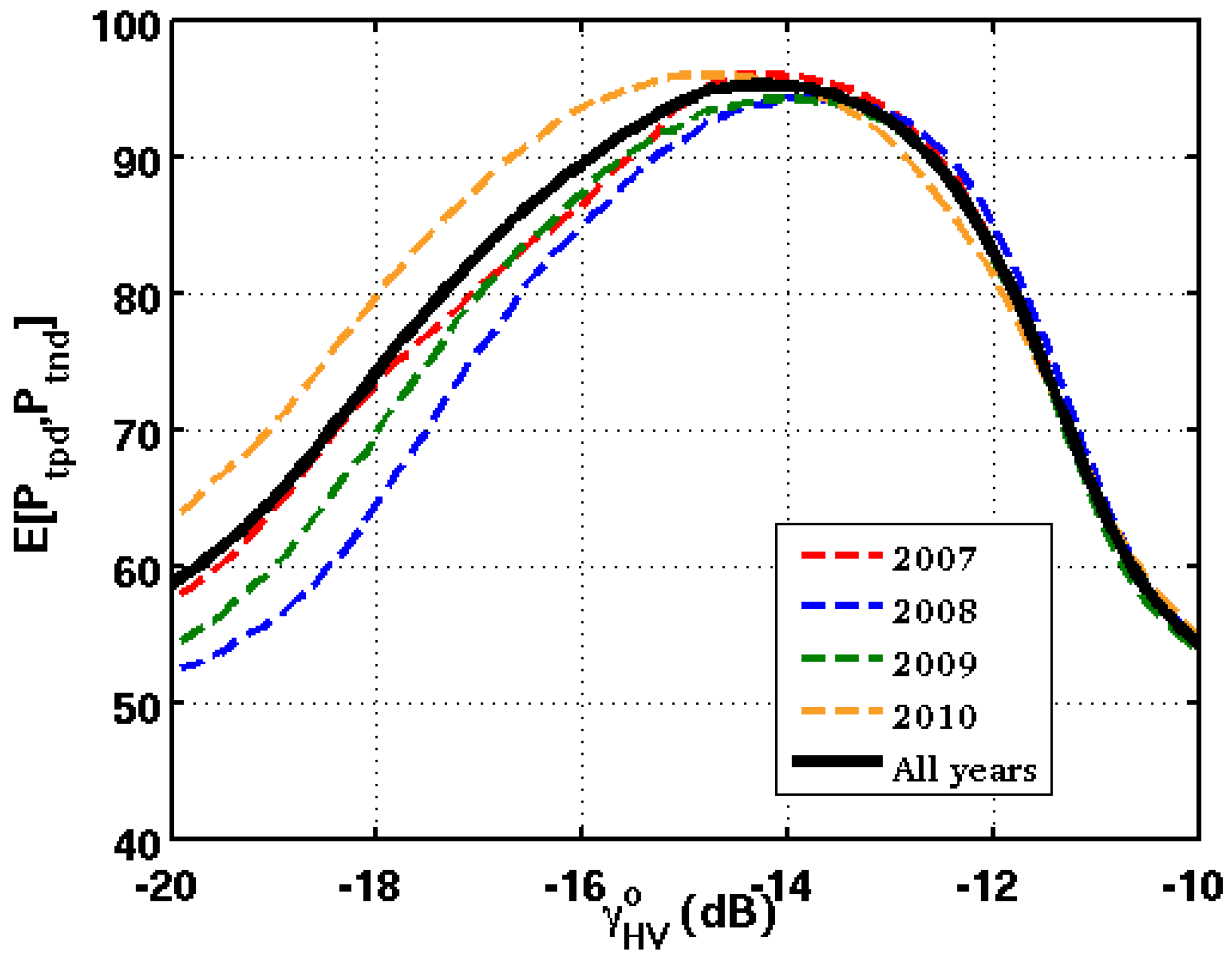
3.4. The EM Algorithm

EM is closely related to fuzzy classification approaches. In EM, each pixel is assigned, with different degrees of class membership, to all possible classes in a way that maximizes the posterior probability of the assignment with respect to a mixture model describing the constellation of classes. It has the advantage of requiring no binary decisions about class memberships; additionally, all possible assignments can be considered in parallel [48,49]. The EM classification algorithm used in this study tries to assign pixels to the three classes, while the optimal set of class centers $\Sigma =({\Sigma }_1,{\Sigma }_2,{\Sigma }_3)$ remains to be found by the classifier. The EM algorithm starts with an initial guess of class centers ${\Sigma }_i^0$. To this end, the sample means for $i=[1,2,3]$ are estimated as maximum-likelihood estimates of the unknown real ${\Sigma }_i^0$:

$${\displaystyle {\Sigma }_i^0=\frac{1}{N_i}\sum _{\mathit{\nu }\in {\omega }_i}R\left(\mathit{\nu }\right)}$$

(8)

where $N_i$ is the number of pixels in ${\omega }_i$. Initial seed regions can be randomly selected or manually determined. Then, the a posteriori probabilities $p_{\mathit{\nu },i}^k$ that a pixel belongs to class i, given its ratio $R\left(\mathit{\nu }\right)$ and the set of class centers $({\Sigma }_1^0,{\Sigma }_2^0,{\Sigma }_3^0)$, are estimated in the so-called expectation step:

$$\begin{array}{cc}& p_{\mathit{\nu },i}^k=\frac{p(R\left(\mathit{\nu }\right)\setminus {\Sigma }_i^k)}{{\displaystyle \sum _{j=1}^3}p(R\left(\mathit{\nu }\right)\setminus {\Sigma }_j^k)}\hfill \\ & {\displaystyle p_{\mathit{\nu },i}^k\in [0,1]\forall \mathit{\nu },i\text{and}\sum _{i=1}^3{p}_{\mathit{\nu },i}^k=1\forall i}\hfill \end{array}$$

(9)

where k is the current iteration step. Using the estimated $p_{\mathit{\nu },i}^k$, an updated set of class centers can be assessed in the next maximization step:

$${\displaystyle {\Sigma }_i^{k+1}=\frac{{\displaystyle \sum _{\mathit{\nu }=1}^N{p}_{\mathit{\nu },i}^{k}R\left(\mathit{\nu }\right)}}{{\displaystyle \sum _{\mathit{\nu }=1}^N{p}_{\mathit{\nu },i}^k}}}$$

(10)

The EM algorithm stops when a certain termination criterion is met. In this study, we chose the convergence of class centers between two subsequent iterations:

$$\frac{1}{N}\sqrt{{\displaystyle \sum _{\mathit{\nu },i}{({\Sigma }_i^{k+1}-{\Sigma }_i^k)}^2}}$$

(11)

If the difference between two subsequent class centers falls below 1% for each class, the iteration process stops, and each pixel is assigned to the most likely class, following the decision:

$$\mathit{\nu }\in {\omega }_i\text{if}{p}_{\mathit{\nu },i}^k>p_{\mathit{\nu },j}^k\forall j$$

(12)

3.5. The Forest Disturbances and Regrowth Detection Algorithm

We decided to perform the forest disturbance detection at a one-year temporal frequency using data acquired between 2007 and 2008, 2008 and 2009 and 2009 and 2010, i.e., three times, to observe the temporal evolution of the disturbances. The forest regrowth detection was achieved over a three-year interval using data acquired between 2007 and 2010, i.e., once, because the regrowth phenomenon is slow, and its detection at a temporal frequency of one year would be strongly affected by error. For each time, a pixel is assigned to the forest disturbance or regrowth class if:

• The pixel was not masked by the procedure described in Section 3.2;
• The condition in Equation (12) is fulfilled;
• ${\gamma }_{HV}\ge -14$ dB before the forest disturbance event and ${\gamma }_{HV}<-14$ dB after the forest disturbance event for forest disturbance class; and
• ${\gamma }_{HV}<-14$ dB before the forest regrowth event and ${\gamma }_{HV}\ge -14$ dB after the forest regrowth event for the forest regrowth class.

The threshold $-14$ dB has been chosen because it corresponds to the best average between the true positive and true negative detection probabilities when classifying forest and non-forest areas, as explained in Section 4.2.

In this study, the disturbances or regrowth rates (r) are calculated according to the equation from [50]:

$$r=\frac{1}{t_2-t_1}.ln(\frac{A_2}{A_1})$$

(13)

where $A_1$ and $A_2$ are the forest areas at time $t_1$ and $t_2$, respectively.

A flowchart summarizing the forest disturbances and regrowth detection method is shown in Figure 4.

3.6. Uncertainties Assessment

3.6.1. Uncertainties Related to Areas of Forest Disturbance

To assess uncertainties related to areas of forest disturbance, we applied the method presented in [51]. This method takes advantage of the map and accuracy assessment data by: (1) estimating accuracy (e.g., user’s, producer’s and overall accuracies); (2) estimating the area of forest disturbances and regrowth using the accuracy assessment sample data to adjust the area for map classification errors; and (3) estimating confidence intervals for the error-adjusted area estimates. The confidence interval provides a range of values for the area of forest disturbances and regrowth, taking into account the uncertainty of the sample-based estimate (e.g., the estimation of the accuracy from the database defined in Section 2.3). Other sources of uncertainty exist, but are minimized by using a SAR data processing particularly suited for change detection (Section 3.1) and by masking areas that may exhibit SAR backscatter that could be incorrectly interpreted as disturbed forest or regrowth (Section 3.2). Note that we did not propagate in the forest disturbance and regrowth detection algorithm the error related to the backscatter because of the presence of speckle noise to avoid excessive computational time. In addition, this error may be considered to be small (in Section 3.1, we estimated the standard deviation of the backscatter to be approximately 0.4 dB after SAR data pre-processing) relative to the intensity ratio of a disturbance event (mean > 5 dB, as shown in the next Section 4.1).

In this paper, the rows of the error matrix show the intact forest (Intact), the annual forest disturbances between 2007 and 2008, 2008 and 2009 and 2009 and 2010, and the forest regrowth between 2007 and 2010 (where i ranges from one to five), as assigned by the detection method. The columns indicate the reference polygons from the database derived as explained in Section 2.2 (where j ranges from one to five). We estimate the error matrix of the estimated area proportions ${\tilde{p}}_{ij}$ from the error matrix of the sample counts $n_{ij}$ as follows:

$${\tilde{p}}_{ij}=W_i\frac{n_{ij}}{n_{i.}}$$

(14)

where $W_i$ is the proportion of the area mapped as class i relative to the total area $A_{tot}$ and $n_{i.}$ is the sum of the samples in row i in the error matrix of the sample counts. In the results section, we report the areas of forest disturbances and regrowth that were obtained directly from the map classification (which are usually biased) and also present an unbiased estimation of these areas (${\tilde{A}}_j$ for the estimated area of class j) following [51]:

$${\tilde{A}}_j=A_{tot}.\sum _i{W}_i\frac{n_{ij}}{n_{i.}}$$

(15)

The estimated standard error of the estimated area proportion for class j is [52]:

$$S\left({\tilde{p}}_{.j}\right)=\sqrt{\sum _{i=1}^5{W}_i^2\frac{\frac{n_{ij}}{n_{i.}}(1-\frac{n_{ij}}{n_{i.}}}{n_{i.}-1}}$$

(16)

where ${\tilde{p}}_{.j}$ is the sum of the samples in column j in the error matrix of the estimated area proportions. The standard error of the error-adjusted estimated area is:

$$S({\tilde{A}}_j)=A_{tot}.S\left({\tilde{p}}_{.j}\right)$$

(17)

The approximate 95% confidence interval for $A_j$ is $2\times S({\tilde{A}}_j)$.

3.6.2. Uncertainties Related to Carbon Emission Estimates

From the obtained disturbed areas, we estimated AGB loss using the AGB values from the maps of Saatchi et al. [53] and Baccini et al. [54]. The former provide a continuous uncertainty map, whereas the latter do not provide a pixel-level uncertainty map. When assessing AGB loss using the map from [53], we also used their uncertainty map. Because the uncertainty map includes uncertainties (shown as ${ϵ}_{tot,\mathit{\nu }}$) associated with AGB and below-ground biomass (BGB) at pixel position ν, we calculated the error related to AGB only:

$${ϵ}_{AGB,\mathit{\nu }}=\sqrt{\frac{{ϵ}_{tot,\mathit{\nu }}^2-23.2^2}{1+0.{89}^2}}$$

(18)

Relative errors at the regional scale (shown as ${ϵ}_{AGB,reg}$) are computed by summing the errors from all pixels:

$${ϵ}_{AGB,reg}=\sqrt{\frac{{\sum }_{i=1}^N{(AG{B}_i.{ϵ}_{AGB,i})}^2}{{\sum }_{i=1}^{N}AG{B}_i}}$$

(19)

where $AG{B}_i$ is the AGB at pixel i and N the number of pixels in the region.

3.6.3. Propagation of Uncertainties

Errors related to the areas of forest disturbances and Saatchi’s map [53] were propagated by Monte Carlo simulations (1000 simulations) to yield a standard deviation associated with the AGB loss estimates. For these simulations, these errors were assumed to follow a normal distribution. For each simulation, the errors were randomly and independently drawn from the error distributions, and a new AGB loss estimate was calculated. We finally calculated the standard deviation of the AGB loss based on 1000 AGB replicates.

4. Results and Discussion

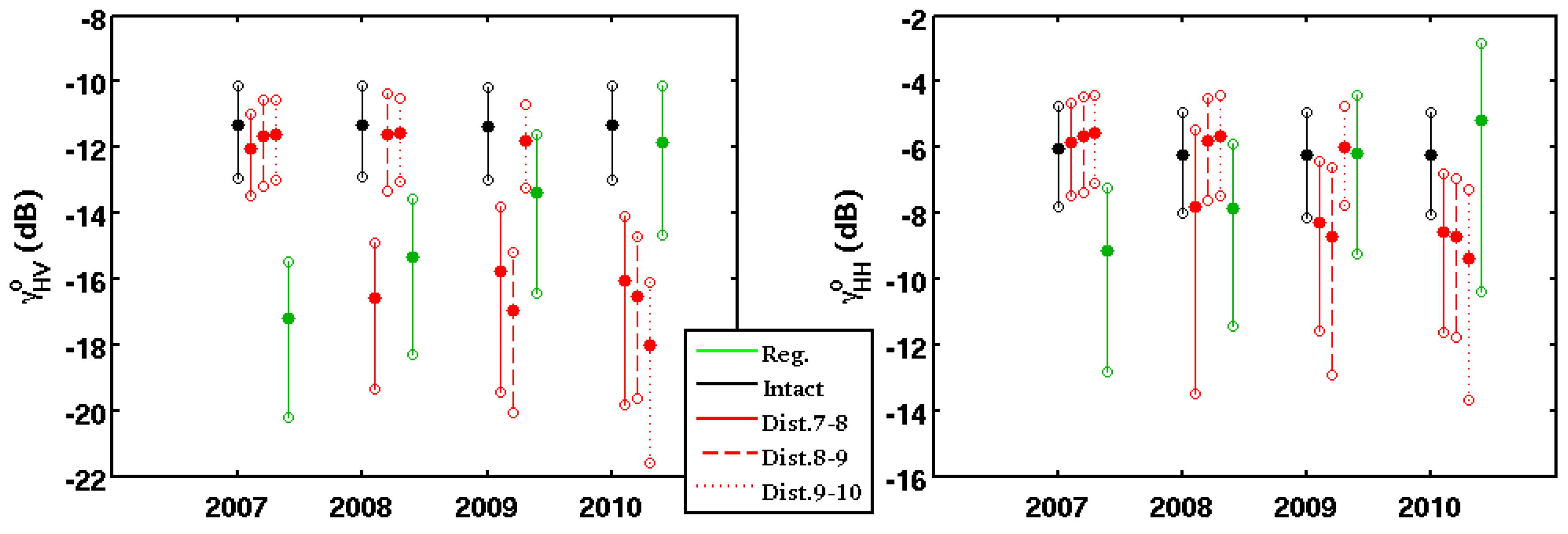
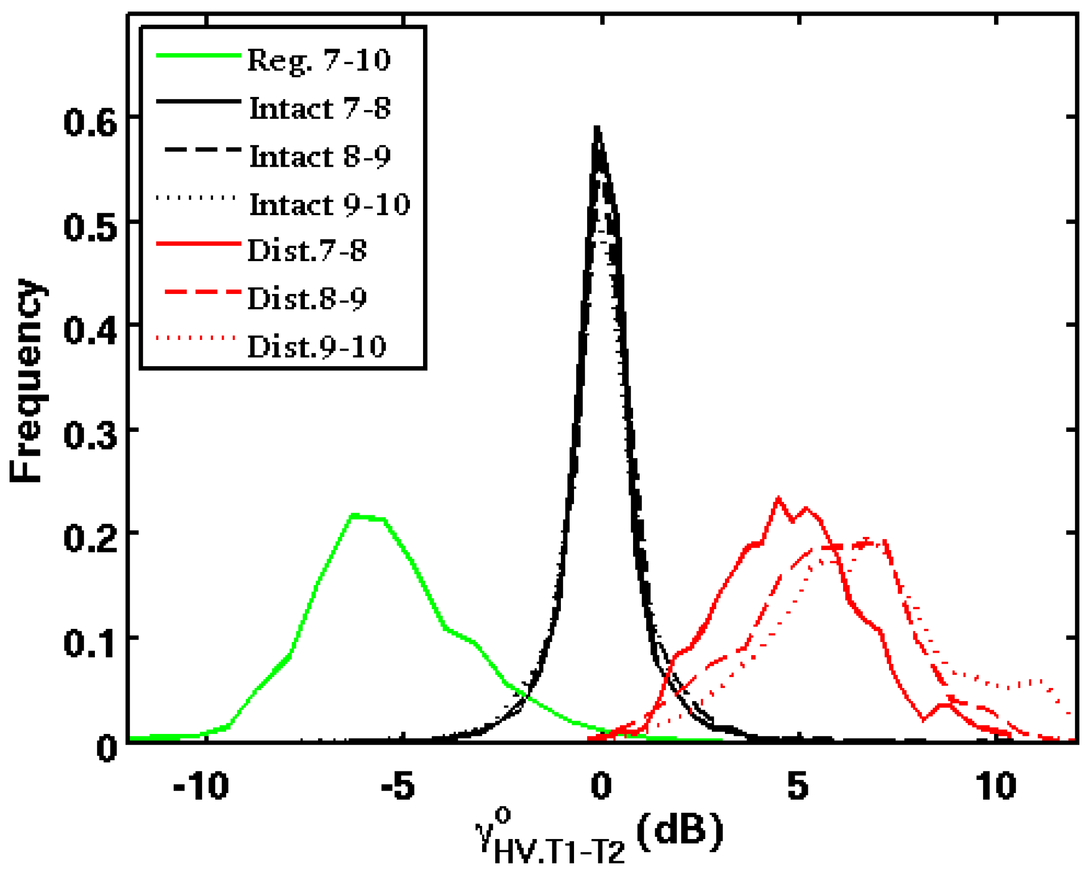
4.1. Characteristics of Backscatter for Natural Forest, Disturbed and Regrowth Areas

Distributions of the intensity ratio R based on ${\gamma }_{HV}$ are presented in Figure 5 over intact forest, disturbed areas and regrowth areas. Between 2007 and 2008, 2008 and 2009 and 2009 and 2010, the distributions of disturbed areas showed mean R values of $5.18\pm 1.65$, $6.57\pm 5.85$ and $7.28\pm 2.04$ dB, respectively, whereas the distributions of intact forest showed values of $0.12\pm 1.00$, $0.22\pm 1.30$ and $0.13\pm 1.10$ dB, respectively. Regarding forest regrowth, R was $-4.93\pm 2.09$ dB between 2007 and 2010. According to these results, the intensity ratio R of ${\gamma }_{HV}$ is a reliable indicator of forest disturbances and regrowth, even during the wet season.

4.2. Masking Undesirable Areas

Table 2. Masking process results over Vietnam, Cambodia and Lao PDR. Forest and non-forest areas were first separated, and then, terrain slopes 20${}^{\circ }$, inundated lands, mangroves and urban areas were filtered out.

	Vietnam	Cambodia	Lao PDR
Forest (%)	37.9	50.8	58.6
Slope >20${}^{\circ }$ (%)	18.1	1.7	21.7
Inundated lands (%)	2.2	14.3	0.8
Mangroves (%)	0.4	0.3	0
Urban (%)	8.7	9.4	0.6

shows the results of the masking process described in Section 3.2. Pixels were labeled as “forest” when ${\gamma }_{HV}$ exceeded −14 dB, corresponding to the best average between the true positive (93.6%) and true negative (96.7%) detection probabilities, as shown in Figure 6. This threshold is similar to the results in [37] (−14 dB in Sumatra). In total, 37.9%, 50.8% and 58.6% of Vietnam, Cambodia and Lao PDR, respectively, were classified as forest. As a comparison, the General Statistics Office of Vietnam [55] reported forest coverage of 38.7% in 2008 in Vietnam, and the FAO reported 39.7% in 2005 [56]. The FAO also indicated 59.2% forest coverage in Cambodia in 2005 [56]. The difference between the extents of forest coverage estimated by the FAO and here lies in the fact that a large part of the inundated lands masked in Cambodia and, thus, not taken into account in this study, corresponds to an inundated forest located between the city of Battambang and Tonle Sap Lake. This difference would decrease if the forest pixels were extracted during the dry season. The estimation of the forest extent in Lao PDR is more controversial. According to Lao’s Department of Forestry, 41% of Laos was forested in 2011; this value is significantly lower than those estimated by the FAO in 2005 and 2010 (69.9% and 68%, respectively). The 58.6% forest coverage in this study thus represents an intermediate value.

Slopes exceeding 20${}^{\circ }$ represent 18.1% and 21.7% of Vietnam and Lao PDR, respectively, and only 1.7% of Cambodia, which is a relatively flat country. Approximately 14.3% of Cambodia is covered by inundated lands, whereas in Vietnam and Lao PDR, these values are 2.2% and 0.8%, respectively. Mangroves were only noted in Vietnam and Cambodia (0.4% and 0.3%, respectively). Vietnam and Cambodia are also more urbanized than Lao PDR (8.7% and 9.4% versus 0.6%, respectively).

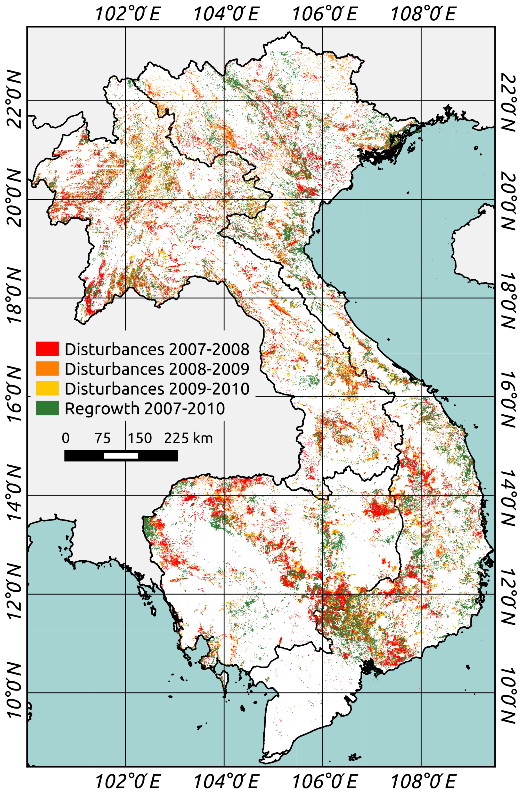
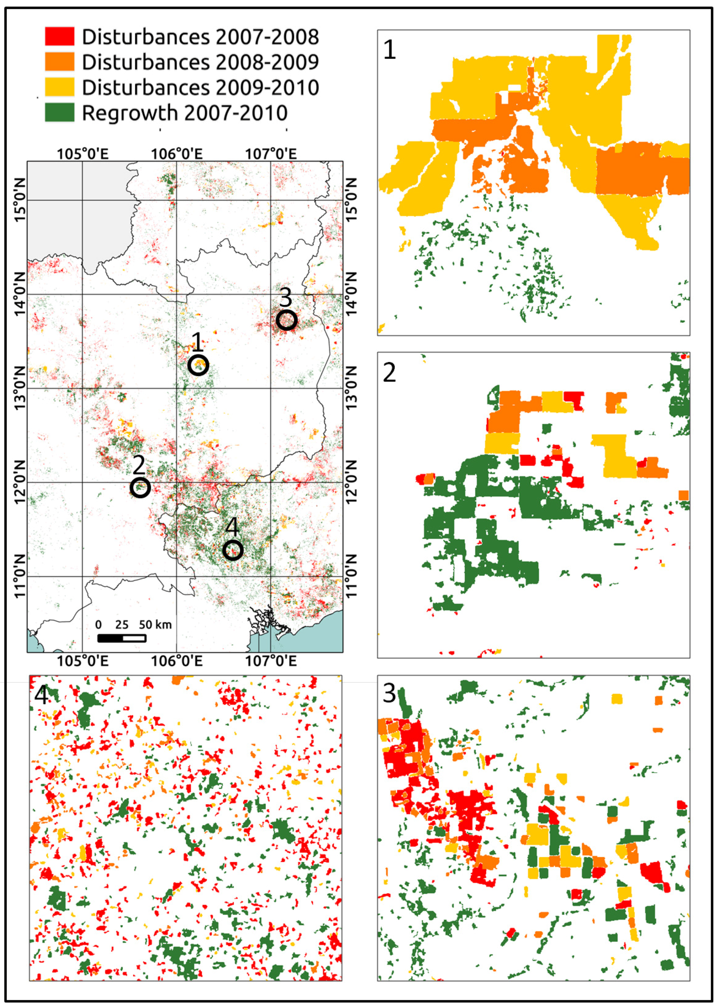
4.3. Forest Disturbances and Regrowth Assessment

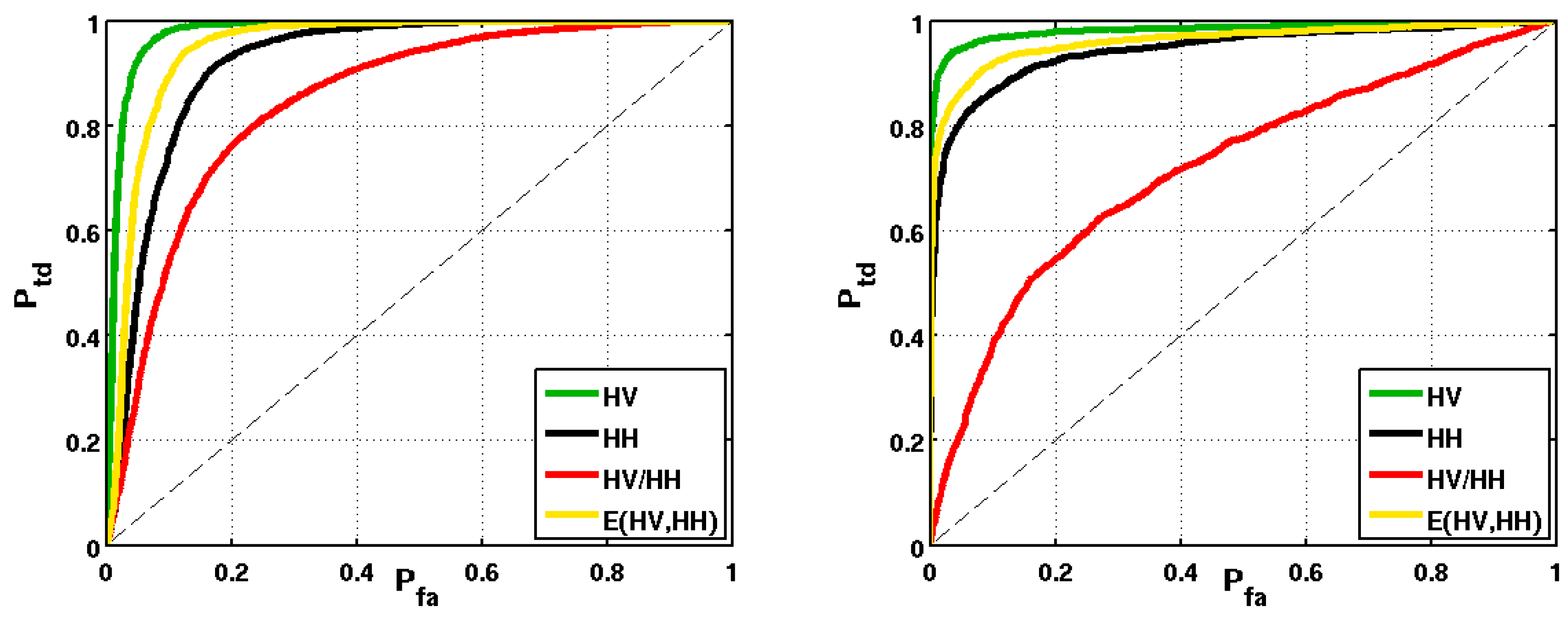
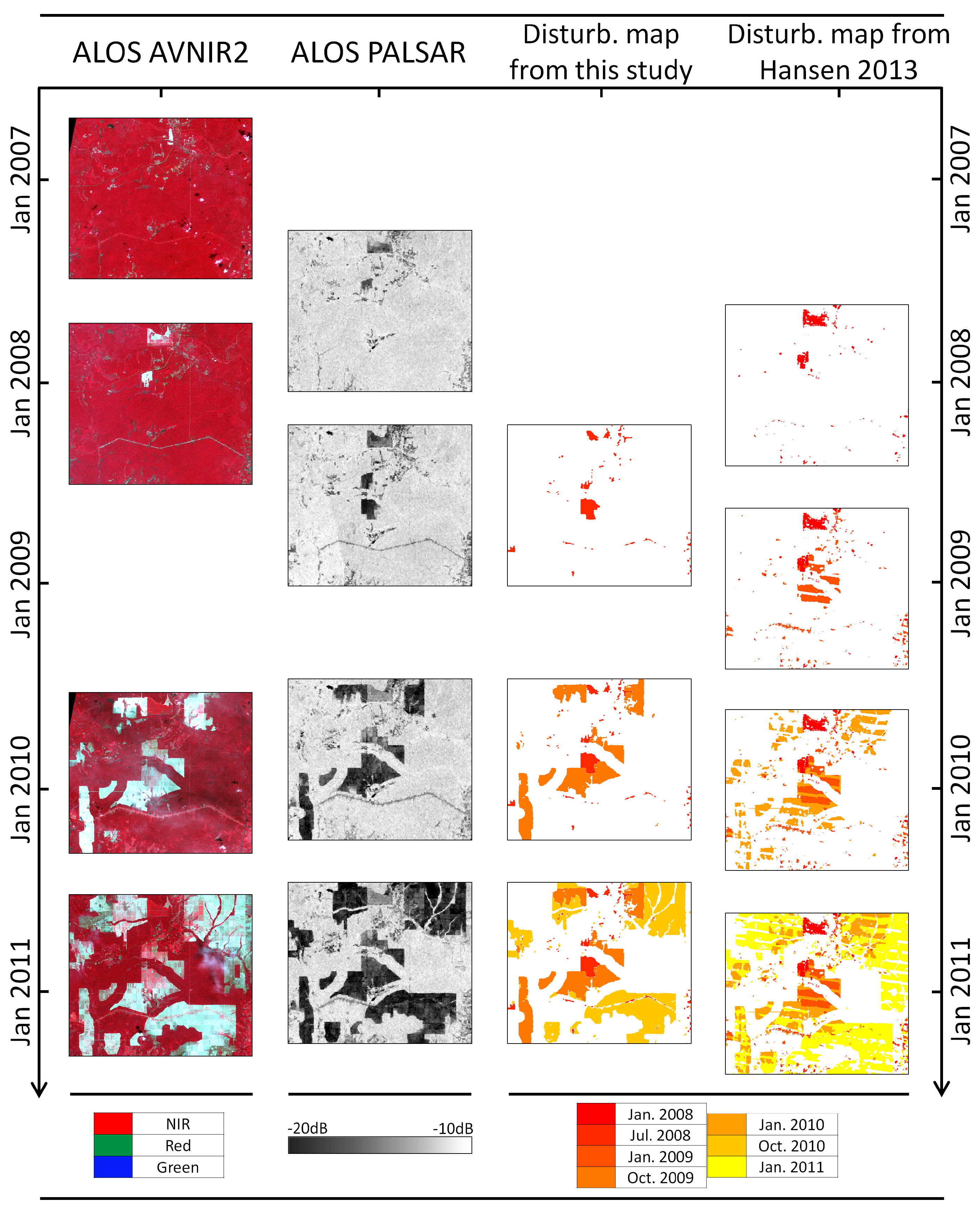
In order to estimate as best as possible forest disturbances and regrowth areas and AGB loss, the whole database has been used to calibrate the proposed forest disturbance and regrowth detection method (whereas two parts of the database are used for calibration and validation in the next Section 4.4 for the evaluation of the method). The proposed forest disturbance and regrowth detection method, detailed in Figure 4, converged after eight iterations according to the termination criterion in Equation (11). The final class centers were ${\Sigma }_1=0.09$ dB, ${\Sigma }_2=3.85$ dB and ${\Sigma }_3=-2.35$ dB. The best results were found using the smallest window ($3\times 3$) required for the estimation of the local mean value. The results slightly decrease as the window size increases. This finding is opposite that of [3], where a surprisingly large window size ($23\times 23$) was required to obtain the best results. The window size is partly related to the characteristic scale of change in the respective region. However, the small window size in our study demonstrates that effective speckle reduction was achieved before the change-detection algorithm was applied, thereby preserving the resolution of the final map without substantial misdetections.

Figure 7 shows the forest disturbances and regrowth maps of Vietnam, Cambodia and Lao PDR between 2007 and 2010. Figure 8, which shows the map in Figure 7 at the pixel scale in $12\times 12$ km areas, highlights the various sizes and distributions of disturbed areas.

The assessment of disturbance rates and regrowth rates is shown in

Table 3. Assessment of the disturbance rates in Vietnam, Cambodia and Lao PDR in this study and by Hansen et al. [9] between 2007 and 2010.

	Vietnam	Cambodia	Lao PDR
Disturb.rates (%)	−1.07	−1.22	−0.94
This study
Disturb. rates (%)	−1.16	−1.58	−0.96
Hansen
Regrowth rates (%)	0.82	0.49	0.35
This study

. For comparison purposes, Table 3 also presents the disturbance rates estimated by [9]. The largest disturbance rate was found to occur in Cambodia (−1.22% in this study and −1.58% in [9]), followed by Vietnam and Lao PDR.

To assess the AGB loss, for the disturbed areas detected by our algorithm, we overlaid the AGB values from the maps of Saatchi et al. [53] and Baccini et al. [54] at the pixel level. However, the level of uncertainty is very high at this small scale. Because the uncertainties that stem from random errors at high levels of estimate aggregation tend to cancel each other out, we also averaged the AGB values and associated uncertainties following Equation (19) over regions in the FAO’s Global Ecological Zones map [57] to assess AGB loss. Paradoxically, the lowest AGB loss (calculated at the pixel level) according to the maps of Saatchi and Baccini was found to occur in Cambodia (59.2 $Tg$ and 43.1 $Tg$, respectively, versus 83.8 $Tg$ and 64 $Tg$ in LAO PDR and 60.7 $Tg$ and 45.2 $Tg$ in Vietnam) because the mean AGB from [53] over Cambodia is lower than those over Vietnam and Lao PDR. The large disturbance rate in Cambodia is not balanced by a significant regrowth rate (0.49%). On the contrary, Vietnam exhibited the greatest regrowth rate (0.82%). In fact, Vietnam has experienced a relative resurgence in forest cover over recent years, mainly because of several internal political, socioeconomic and land-use processes [58]. Additionally, recorded wood imports have increased substantially, and large quantities of illegal logs entered the country, mostly from Cambodia [59] and Lao PDR [60]. Thus, Vietnam outsourced deforestation to Cambodia and Lao PDR [61]. Note that the disturbance rates from [9] systematically exceed those determined here. Bellot et al. [62] reported a similar conclusion, i.e., substantial overestimation of deforestation in Indonesia by [9].

The forest disturbance rates were not found to be geographically homogeneous. In Vietnam, for example, between 2007 and 2010, the southeast region where rubber tree crops have traditionally been grown experienced the largest loss (2438 km${}^2$), followed by the central highlands, which were affected by bauxite mining and the building of hydropower plants (1475 km${}^2$), and the north central coast (1094 km${}^2$). The lowest forest loss occurred in the Mekong River delta (63 km${}^2$), where there is very low forest coverage. The forest disturbance rates were not found to be annually homogeneous. Over Vietnam, the disturbance rates were −1.57%, −0.95% and −0.74% between 2007 and 2008, 2008 and 2009 and 2009 and 2010, respectively. For the same years, the disturbance rates were −1.96%, −0.79% and −0.96% over Cambodia and −1.29%, −0.85% and −0.54% over Lao PDR, respectively. The overall temporal decrease of the forest disturbances could be explained by the global financial crisis in 2008. Following the financial crisis, the global demand for timber decreased, leading to a suspension of plantation clear-cutting. In contrast, the disturbance rates found by [9] increased systematically between 2007 and 2010. In Vietnam, for example, the disturbed forest areas reported by [9] were 1157 km${}^2$, 1427 km${}^2$ and 1814 km${}^2$ between 2007 and 2008, 2008 and 2009 and 2009 and 2010, respectively.

The error-adjusted estimated disturbed, intact and regrowth total areas and associated 95% confidence intervals, calculated following Equations (15) and (17), were 13,523 ± 339 km${}^2$, 368,870 ± 114 km${}^2$ and 6972 ± 77 km${}^2$, respectively. The corresponding total disturbance and regrowth rates are −1.23 ± 0.03% and 0.61% (with a negligible confidence interval), respectively. Using the averaged AGB values and associated uncertainties over regions in the FAO’s Global Ecological Zones map [57], total AGB losses were 269.3 ± 30 $Tg$ and 229.8 ± 5.7 $Tg$ according to Saatchi’s and Baccini’s maps, respectively. Note that the latter do not provide a pixel-level uncertainty map, which explains the lower uncertainty related to AGB losses.

In Figure 9, the temporal series of AVNIR-2 data used to derive the training and testing database (Section 2.3), PALSAR data, our PALSAR-derived forest disturbances and regrowth map and the Landsat-based disturbances map from [9] over a $17\times 15$ km area are visually compared. This example highlights the effect of the Landsat 7 defective scan line corrector, which decreases Hansen’s map quality. Note that Hansen’s map has the merit of being global, unlike the map derived in this study.

4.4. Validation

The forest disturbances and regrowth map was evaluated using an error matrix of sample counts and of estimated area proportions. The area proportions for each class are calculated following Equation (14). In

Table 4. Validation of the forest disturbance and regrowth detection method. In the error matrix of sample counts $n_{ij}$ and of estimated area proportions ${\tilde{p}}_{ij}$ [51] (shown as $n_{ij}/{\tilde{p}}_{ij}$ in the error matrix), rows show the intact forest (Intact), the annual forest disturbances between 2007 and 2008 (Dist.7-8), 2008 and 2009 (Dist.8-9) and 2009 and 2010 (Dist.9-10) and the forest regrowth between 2007 and 2010 (Reg.7-10), as determined by the detection method. Columns indicate the reference polygons from the database derived as explained in Section 2.2. The validation samples represent 90% of the database described in Section 2.3. Based on estimated area proportions, the mean PA was 84.7%, and the mean UA was 96.3%.

		In situ
		Intact	Dist.7-8	Dist.8-9	Dist.9-10	Reg.7-10	UA (%)
Classification	Intact	177,570/0.95	195/1.e${}^{-2}$	266/1.4.e${}^{-3}$	477/2.5.e${}^{-3}$	383/2.e${}^{-3}$	99.3
	Dist.7-8	0/0	963/1.4.e${}^{-2}$	51/7.e${}^{-4}$	48/7.e${}^{-4}$	0/0	90.7
	Dist.8-9	9/10.e${}^{-4}$	3/0	1139/7.7.e${}^{-3}$	78/5.e${}^{-4}$	0/0	92.7
	Dist.9-10	19/0	3/0	6/0	2937/6.7.e${}^{-3}$	0/0	99.1
	Reg.7-10	0/0	0/0	0/0	0/0	1688/1.6.e${}^{-2}$	100
	PA (%)	100	92.8	78	63.9	88.6

, the rows show the different classes (intact forest, forest disturbances and regrowth) assigned by the classifier, whereas the columns indicate the reference polygons derived from the database, as explained in Section 2.3. The training samples represented 10% of the database. The numbers of samples used in the validation step (90% of the database) were 177,598, 1164, 1462, 3540 and 2071 for intact forest, disturbances between 2007 and 2008, 2008 and 2009 and 2009 and 2010 and regrowth between 2007 and 2010, respectively. Based on estimated area proportions, the mean producer’s accuracy (PA) was 84.7%, and the mean user’s accuracy (UA) was 96.3%.

The change map has a PA of intact forest, disturbances between 2007 and 2008 and regrowth of 100%, 92.8% and 88.6%, respectively. The low PAs of 78% and 63.9% for disturbances between 2008 and 2009 and 2009 and 2010 are due to the fact that the proportions of these two classes in the final change map are lower than other classes. In fact, an assessment of the PA for disturbances between 2009 and 2010, based on sample counts, gives a PA of 83%. Note that UA is higher than 90% for all classes.

5. Conclusions

Approximately 15% of the world’s tropical forests are located in Southeast Asia [63]. However, Stibig et al. [23] estimated a drop of the total forest cover of Southeast Asia from approximately 268 Mha in 1990 to 236 Mha in 2010. In this paper, forest disturbances and regrowth in Vietnam, Cambodia and LAO PDR were assessed between 2007 and 2010 using 25-m resolution ALOS PALSAR mosaic data by applying a new semi-automated method that combines SAR data processing, which is particularly suited for change detection from SAR, and EM. A reliable training and testing database was derived from VHR AVNIR-2 and Google Earth images. The forest disturbances and regrowth map indicated disturbance and regrowth rates of −1.23 ± 0.03% and 0.61% (with a negligible confidence interval), respectively. Using the averaged AGB values and associated uncertainties over regions in the FAO’s Global Ecological Zones map [57], total AGB losses were 269.3 ± 30 $Tg$ and 229.8 ± 5.7 $Tg$ according to Saatchi’s and Baccini’s maps, respectively. This study proves that reliable, large-scale maps of forest disturbances and regrowth can be derived using SAR data, even under cloudy weather conditions. This method can be easily applied to other tropical regions using data from ALOS2, which was launched in May 2014, and the P-band Biomass mission planned for 2020.

References

1. Harris, N.L.; Brown, S.; Hagen, S.C.; Saatchi, S.S.; Petrova, S.; Salas, W.; Hansen, M.C.; Potapov, P.V.; Lotsch, A. Baseline map of carbon emissions from deforestation in tropical regions. Science 2012, 336, 1573–1576. [Google Scholar] [CrossRef] [PubMed]
2. Lewis, S.; Lopez-Gonzalez, G.; Sonké, B.; Affum-Baffoe, K.; Baker, T.; Ojo, L.; Phillips, O.; Reitsma, J.; White, L.; Comiskey, J.; et al. Increasing carbon storage in intact African tropical forests. Nature 2009, 457, 1003–1006. [Google Scholar] [CrossRef] [PubMed]
3. Whittle, M.; Quegan, S.; Uryu, Y.; Stüewe, M.; Yulianto, K. Detection of tropical deforestation using ALOS-PALSAR: A sumatran case study. Remote Sens. Environ. 2012, 124, 83–98. [Google Scholar] [CrossRef]
4. Van der Werf, G.R.; Morton, D.C.; DeFries, R.S.; Olivier, J.G.; Kasibhatla, P.S.; Jackson, R.B.; Collatz, G.J.; Randerson, J. CO2 emissions from forest loss. Nat. Geosci. 2009, 2, 737–738. [Google Scholar] [CrossRef]
5. FAO. Global Forest Resources Assessment; Technical Report; Food and Agriculture Association of the United-States: Rome, Italy, 2010. [Google Scholar]
6. Kennedy, R.E.; Yang, Z.; Cohen, W.B. Detecting trends in forest disturbance and recovery using yearly Landsat time series: 1. LandTrendr—Temporal segmentation algorithms. Remote Sens. Environ. 2010, 114, 2897–2910. [Google Scholar] [CrossRef]
7. Cohen, W.B.; Yang, Z.; Kennedy, R. Detecting trends in forest disturbance and recovery using yearly Landsat time series: 2. TimeSync—Tools for calibration and validation. Remote Sens. Environ. 2010, 114, 2911–2924. [Google Scholar] [CrossRef]
8. Zhu, Z.; Woodcock, C.E. Continuous change detection and classification of land cover using all available Landsat data. Remote Sens. Environ. 2014, 144, 152–171. [Google Scholar] [CrossRef]
9. Hansen, M.; Potapov, P.; Moore, R.; Hancher, M.; Turubanova, S.; Tyukavina, A.; Thau, D.; Stehman, S.; Goetz, S.; Loveland, T.; et al. High-resolution global maps of 21st-century forest cover change. Science 2013, 342, 850–853. [Google Scholar] [CrossRef] [PubMed]
10. Sannier, C.; McRoberts, R.E.; Fichet, L.V. Suitability of global forest change data to report forest cover estimates at national level in Gabon. Remote Sens. Environ. 2015, 173, 326–338. [Google Scholar] [CrossRef]
11. Holmgren, P. Can we trust country-level data from global forest assessments? For. News. 2015. Available online: http://blog.cifor.org/34669/ (accessed on 1 December 2015).
12. Le Toan, T.; Beaudoin, A.; Riom, J.; Guyon, D. Relating forest biomass to SAR data. Geosci. Remote Sens. IEEE Trans. 1992, 30, 403–411. [Google Scholar] [CrossRef]
13. Le Toan, T.; Quegan, S.; Woodward, I.; Lomas, M.; Delbart, N.; Picard, G. Relating radar remote sensing of biomass to modelling of forest carbon budgets. Clim. Chang. 2004, 67, 379–402. [Google Scholar] [CrossRef]
14. Mermoz, S.; Réjou-Méchain, M.; Villard, L.; Le Toan, T.; Rossi, V.; Gourlet-Fleury, S. Decrease of L-band SAR backscatter with biomass of dense forests. Remote Sens. Environ. 2015, 159, 307–317. [Google Scholar] [CrossRef]
15. Santos, J.; Lacruz, M.; Araujo, L.; Keil, M. Savanna and tropical rainforest biomass estimation and spatialization using JERS-1 data. Int. J. Remote Sens. 2002, 23, 1217–1229. [Google Scholar] [CrossRef]
16. Santoro, M. Estimation of Biophysical Parameters in Boreal Forests from ERS and JERS SAR Interferometry. Ph.D. Thesis, Department of Radio and Space Science, Chalmers University of Technology, GÃ˝uteborg, Sweden, 2003. [Google Scholar]
17. Saatchi, S.; Marlier, M.; Chazdon, R.; Clark, D.; Russell, A. Impact of spatial variability of tropical forest structure on radar estimation of aboveground biomass. Remote Sens. Environ. 2011, 115, 2836–2849. [Google Scholar] [CrossRef]
18. Cartus, O.; Santoro, M.; Kellndorfer, J. Mapping forest aboveground biomass in the Northeastern United States with ALOS PALSAR dual polarization L-band. Remote Sens. Environ. 2012, 124, 466–478. [Google Scholar] [CrossRef]
19. Carreiras, J.; Melo, J.B.; Vasconcelos, M.J. Estimating the above-ground biomass in Miombo Savanna woodlands (Mozambique, East Africa) using L-band synthetic aperture radar data. Remote Sens. 2013, 5, 1524–1548. [Google Scholar] [CrossRef]
20. Mermoz, S.; Le Toan, T.; Villard, L.; Réjou-Méchain, M.; Seifert-Granzin, J. Biomass assessment in the Cameroon savanna using ALOS PALSAR data. Remote Sens. Environ. 2014, 155, 109–119. [Google Scholar] [CrossRef]
21. Shimada, M.; Itoh, T.; Motooka, T.; Watanabe, M.; Shiraishi, T.; Thapa, R.; Lucas, R. New global forest/non-forest maps from ALOS PALSAR data (2007–2010). Remote Sens. Environ. 2014. [Google Scholar] [CrossRef]
22. Achard, F.; Eva, H.; Stibig, H.; Mayaux, P.; Gallego, J.; Richards, T.; Malingreau, J. Determination of deforestation rates of the world’s humid tropical forests. Science 2002, 297, 999–1002. [Google Scholar] [CrossRef] [PubMed]
23. Stibig, H.; Achard, F.; Carboni, S.; Raši, R.; Miettinen, J. Change in tropical forest cover of Southeast Asia from 1990 to 2010. Biogeosciences 2014, 11, 247–258. [Google Scholar] [CrossRef] [Green Version]
24. Liao, C.; Luo, Y.; Fang, C.; Li, B. Ecosystem carbon stock influenced by plantation practice: implications for planting forests as a measure of climate change mitigation. PLoS ONE 2010, 5, e10867. [Google Scholar] [CrossRef] [PubMed]
25. Nizami, S.M.; Yiping, Z.; Liqing, S.; Zhao, W.; Zhang, X. Managing carbon sinks in rubber (Hevea brasilensis) plantation by changing rotation length in SW China. PLoS ONE 2014, 9, e115234. [Google Scholar] [CrossRef] [PubMed]
26. Witness, G. Rubber barons. In How Vietnamese Companies and International Financers are Driving a Land Grabbing Crisis in Cambodia and Laos. London; Global Witness Limited: London, UK, 2013. [Google Scholar]
27. Moser, G.; Serpico, S.; Vernazza, G. Unsupervised change detection from multichannel SAR images. Geosci. Remote Sens. Lett. IEEE 2007, 4, 278–282. [Google Scholar] [CrossRef]
28. Bazi, Y.; Melgani, F.; Bruzzone, L.; Vernazza, G. A genetic expectation-maximization method for unsupervised change detection in multitemporal SAR imagery. Int. J. Remote Sens. 2009, 30, 6591–6610. [Google Scholar] [CrossRef]
29. Reigber, A.; Jäger, M.; Neumann, M.; Ferro-Famil, L. Classifying polarimetric SAR data by combining expectation methods with spatial context. Int. J. Remote Sens. 2010, 31, 727–744. [Google Scholar] [CrossRef]
30. Shimada, M.; Isoguchi, O.; Tadono, T.; Isono, K. PALSAR radiometric and geometric calibration. Geosci. Remote Sens. IEEE Trans. 2009, 47, 3915–3932. [Google Scholar] [CrossRef]
31. Google. Google Earth 7; Google Inc.: Mountain View, CA, USA, 2011. [Google Scholar]
32. Dorais, A.; Cardille, J. Strategies for incorporating high-resolution google earth databases to guide and validate classifications: Understanding deforestation in Borneo. Remote Sens. 2011, 3, 1157–1176. [Google Scholar] [CrossRef]
33. Radke, R.J.; Andra, S.; Al-Kofahi, O.; Roysam, B. Image change detection algorithms: A systematic survey. Image Proc. IEEE Trans. 2005, 14, 294–307. [Google Scholar] [CrossRef]
34. Shimada, M.; Ohtaki, T. Generating large-scale high-quality SAR mosaic datasets: Application to PALSAR data for global monitoring. Geosci. Remote Sens. IEEE Trans. 2010, 3, 637–656. [Google Scholar] [CrossRef]
35. Bruniquel, J.; Lopes, A. Multi-variate optimal speckle reduction in SAR imagery. Int. J. Remote Sens. 1997, 18, 603–627. [Google Scholar] [CrossRef]
36. Quegan, S.; Yu, J. Filtering of multichannel SAR images. Geosci. Remote Sens. IEEE Trans. 2001, 39, 2373–2379. [Google Scholar] [CrossRef]
37. Motohka, T.; Shimada, M.; Uryu, Y.; Setiabudi, B. Using time series PALSAR gamma nought mosaics for automatic detection of tropical deforestation: A test study in Riau, Indonesia. Remote Sens. Environ. 2014, 155, 79–88. [Google Scholar] [CrossRef]
38. Du, Y.; Cihlar, J.; Beaubien, J.; Latifovic, R. Radiometric normalization, compositing, and quality control for satellite high resolution image mosaics over large areas. Geosc. Remote Sens. IEEE Trans. 2001, 39, 623–634. [Google Scholar]
39. Giri, C.; Ochieng, E.; Tieszen, L.; Zhu, Z.; Singh, A.; Loveland, T.; Masek, J.; Duke, N. Status and distribution of mangrove forests of the world using earth observation satellite data. Glob. Ecol. Biogeogr. 2011, 20, 154–159. [Google Scholar] [CrossRef]
40. Danko, D.M. The digital chart of the world project. Photogramm. Eng. Remote Sens. 1992, 58, 1125–1128. [Google Scholar]
41. Sexton, J.O.; Song, X.P.; Feng, M.; Noojipady, P.; Anand, A.; Huang, C.; Kim, D.H.; Collins, K.M.; Channan, S.; DiMiceli, C.; et al. Global, 30-m resolution continuous fields of tree cover: Landsat-based rescaling of MODIS vegetation continuous fields with lidar-based estimates of error. Int. J. Digit. Earth 2013, 6, 427–448. [Google Scholar] [CrossRef]
42. Bontemps, S.; Defourny, P.; Van Bogaert, E.; Arino, O.; Kalogirou, V.; Ramos Perez, J. GlobCover 2009: Products Description and Validation Report. 2011, Volume 2. Available online: http://ionia1.esrin.esa. int/docs/GLOBCOVER2009_Validation_Report_2 (accessed on 1 December 2015).
43. Bujor, F.; Trouvé, E.; Valet, L.; Nicolas, J.M.; Rudant, J.P. Application of log-cumulants to the detection of spatiotemporal discontinuities in multitemporal SAR images. Geosci. Remote Sens. IEEE Trans. 2004, 42, 2073–2084. [Google Scholar] [CrossRef]
44. Inglada, J.; Mercier, G. A new statistical similarity measure for change detection in multitemporal SAR images and its extension to multiscale change analysis. Geosci. Remote Sens. IEEE Trans. 2007, 45, 1432–1445. [Google Scholar] [CrossRef]
45. Santoro, M.; Fransson, J.E.; Eriksson, L.E.; Ulander, L.M. Clear-cut detection in Swedish boreal forest using multi-temporal ALOS PALSAR backscatter data. Sel. Top. Appl. Earth Obs. Remote Sens. IEEE J. 2010, 3, 618–631. [Google Scholar] [CrossRef]
46. Joshi, N. P.; Mitchard, E. T.; Schumacher, J.; Johannsen, V.K.; Saatchi, S.; Fensholt, R. L-band SAR backscatter related to forest cover, height and aboveground biomass at multiple spatial scales across Denmark. Remote Sens. 2015, 7, 4442–4472. [Google Scholar] [CrossRef]
47. Zadeh, L.A. Fuzzy logic and approximate reasoning. Synthese 1975, 30, 407–428. [Google Scholar] [CrossRef]
48. Bezdek, J.C. Pattern Recognition with Fuzzy Objective Function Algorithms; Plenum press: New York, NY, United States, 1981. [Google Scholar]
49. Du, L.; Lee, J. Fuzzy classification of earth terrain covers using complex polarimetric SAR data. Int. J. Remote Sens. 1996, 17, 809–826. [Google Scholar] [CrossRef]
50. Puyravaud, J.P. Standardizing the calculation of the annual rate of deforestation. For. Ecol. Manag. 2003, 177, 593–596. [Google Scholar] [CrossRef]
51. Olofsson, P.; Foody, G.M.; Stehman, S.V.; Woodcock, C.E. Making better use of accuracy data in land change studies: Estimating accuracy and area and quantifying uncertainty using stratified estimation. Remote Sens. Environ. 2013, 129, 122–131. [Google Scholar] [CrossRef]
52. Cochran, W.G. Sampling Techniquess; Wiley: New York, NY, USA, 1977. [Google Scholar]
53. Saatchi, S.S.; Harris, N.L.; Brown, S.; Lefsky, M.; Mitchard, E.T.; Salas, W.; Zutta, B.R.; Buermann, W.; Lewis, S.L.; Hagen, S.; et al. Benchmark map of forest carbon stocks in tropical regions across three continents. Proc. Natl. Acad. Sci. 2011, 108, 9899–9904. [Google Scholar] [CrossRef] [PubMed]
54. Baccini, A.; Goetz, S.; Walker, W.; Laporte, N.; Sun, M.; Sulla-Menashe, D.; Hackler, J.; Beck, P.; Dubayah, R.; Friedl, M.; et al. Estimated carbon dioxide emissions from tropical deforestation improved by carbon-density maps. Nat. Clim. Chang. 2012, 2, 182–185. [Google Scholar] [CrossRef]
55. General Statistics Office of Vietnam. Agriculture, Fishery and Fishery Statistical Data. Available online: http://www.gso.gov.vn/ (accessed on 1 December 2015).
56. FAO. Global Forest Resources Assessment; Technical Report; Food and Agriculture Association of the United-States: Rome, Italy, 2005. [Google Scholar]
57. Iremonger, S.; Gerrand, A.M. Global Ecological Zones Map for FAO FRA 2010; Technical Report; FAO: Rome, Italy, 2011. [Google Scholar]
58. Lang, C. The Pulp Invasion: The International Pulp and Paper Industry in the Mekong Region; World Rainforest Movement Montevideo: Moreton-in-Marsh, UK, 2002. [Google Scholar]
59. EIA-Telepak. Borderlines: Vietnam’s Booming Furniture Industry and Timber Smuggling in the Mekong Region; Technical Report; Environmental Investigation Agency-Telapak: London, UK, 2008. [Google Scholar]
60. Grainger, A. Difficulties in tracking the long-term global trend in tropical forest area. Proc. Natl. Acad. Sci. 2008, 105, 818–823. [Google Scholar] [CrossRef] [PubMed]
61. Meyfroidt, P.; Lambin, E.F. Forest transition in Vietnam and displacement of deforestation abroad. Proc. Natl. Acad. Sci. 2009, 106, 16139–16144. [Google Scholar] [CrossRef] [PubMed]
62. Bellot, F.; Bertram, M.; Navratil, P.; Siegert, F.; Dotzauer, H. The High Resolution Global Map of 21st Century Forest Cover Change from the University of Maryland is Hugely Overestimating Deforestation in Indonesian; Technical Report; Forests and Climate Change Programme (FORCLIME): Jakarta, Indonesia, 2014. [Google Scholar]
63. FAO. Global Forest Resources Assessment; Technical Report; Food and Agriculture Association of the United-States: Rome, Italy, 1995. [Google Scholar]
Figure 1. Polygons of natural, disturbed and regrowth forest areas in Vietnam, Cambodia and Lao PDR between 2007 and 2010 drawn by visual interpretation of high- and very high-resolution optical images superposed over HV-polarized 2010 ALOS mosaics.
Remotesensing 08 00217 g001
Figure 2. PALSAR multi-temporal γ H V and γ H H for intact forest, disturbed areas between 2007 and 2008 (Dist.7–8), 2008 and 2009 (Dist.8–9) and 2009 and 2010 (Dist.9–10) and regrowth areas between 2007 and 2010 (Reg.), calculated using the database described in Section 2.3. The average (filled point) and standard deviation (vertical bar) are shown.
Remotesensing 08 00217 g002
Figure 3. Receiver operating characteristic (ROC) plot comparison of γ H V , γ H H , γ H V / γ H H and E( γ H V , γ H H ), where E is the average value. (left) Forest disturbances versus intact forest detection; and (right) forest regrowth versus intact forest detection.
Remotesensing 08 00217 g003
Figure 4. Flowchart representing the forest disturbances and regrowth detection method. SRTM DEM is the Shuttle Radar Topography Mission digital elevation model; WCMC WMD is the World Conservation Monitoring Centre world map of mangrove distribution; and PD is the probability density. H V 1 is the average intensity at Date 1; R ( ν ) = H V 1 ( ν ) | H V 2 ( ν ) is the intensity ratio of a homogeneous region centered at pixel position ν in the image; Σ i k is the mean ratio of class ω i ; and k is the current iteration step.
Remotesensing 08 00217 g004
Figure 5. Distributions of the intensity ratio R based on γ H V drawn over intact forest between 2007 and 2008 (Intact. 7–8), 2008 and 2009 (Intact. 8–9) and 2009 and 2010 (Intact. 9–10), disturbed areas between 2007 and 2008 (Dist. 7–8), 2008 and 2009 (Dist. 8–9) and 2009 and 2010 (Dist. 9–10) and regrowth areas between 2007 and 2010 (Reg. 7–10). R based on γ H V is a reliable indicator of forest disturbance and regrowth, even during the wet season.
Remotesensing 08 00217 g005
Figure 6. Average between true positive p t p d and true negative p t n d forest detection with varying thresholds applied to γ H V using ALOS PALSAR data between 2007 and 2010. The bold line represents the whole period.
Remotesensing 08 00217 g006
Figure 7. Forest disturbances and regrowth maps between 2007 and 2010 over Vietnam, Cambodia and Lao PRD at 25-m resolution.
Remotesensing 08 00217 g007
Figure 8. Forest disturbances and regrowth maps between 2007 and 2010 at 25-m resolution over 12 × 12 km areas in Cambodia and Vietnam, highlighting the various sizes and distributions of disturbed and regrowth areas.
Remotesensing 08 00217 g008
Figure 9. Visual comparison of the temporal series of AVNIR-2 data used to derive the training and testing database (Section 2.3), PALSAR data, our PALSAR-derived forest disturbances and regrowth map and the Landsat-based disturbances map from [9]. The 17 × 15 km scene is centered at ∼12.56 N–105.46 E. This example highlights the effect of the Landsat 7 defective scan line corrector, which decreased Hansen’s map quality.
Remotesensing 08 00217 g009