
The Optimal Leaf Biochemical Selection for Mapping Species Diversity Based on Imaging Spectroscopy


Abstract
:
1. Introduction
2. Materials
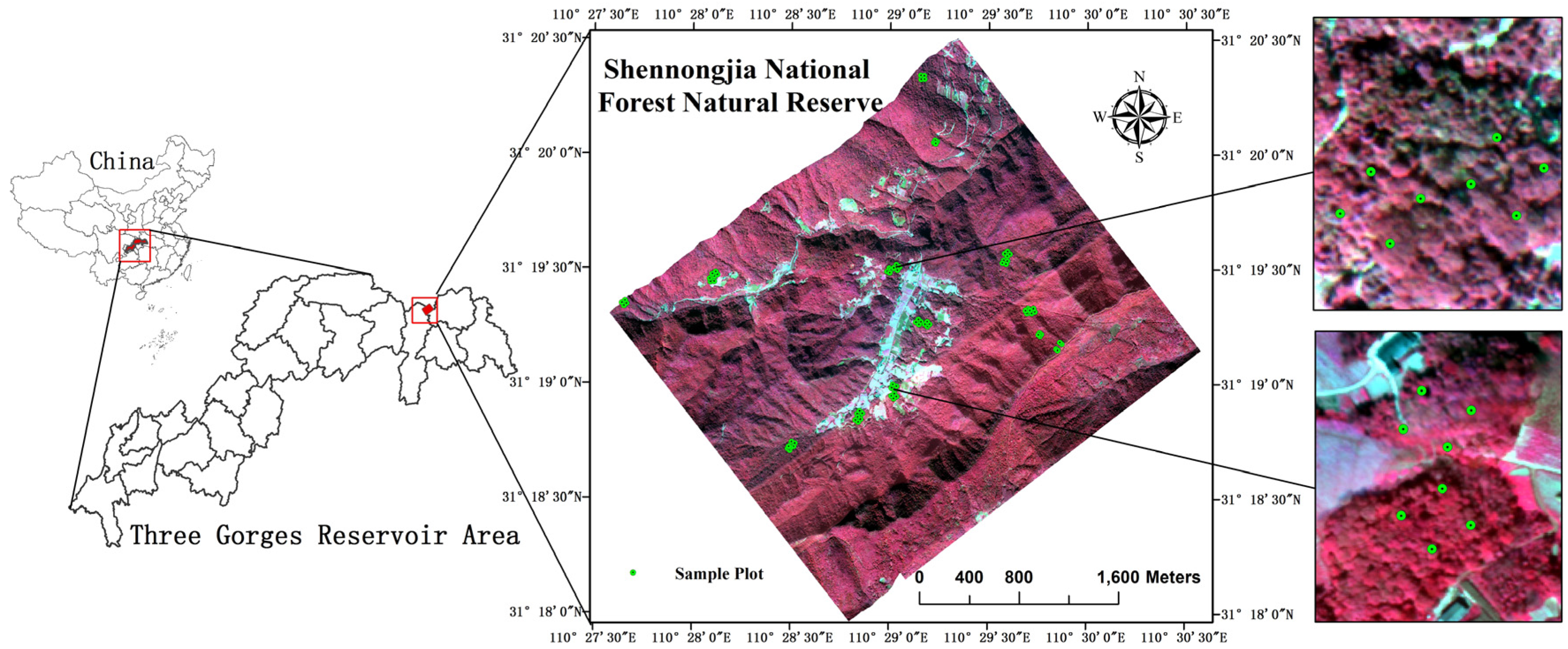
2.1. Study Site
2.2. Field Biochemical and Spectral Data
2.3 Statistical Analysis
3. Results
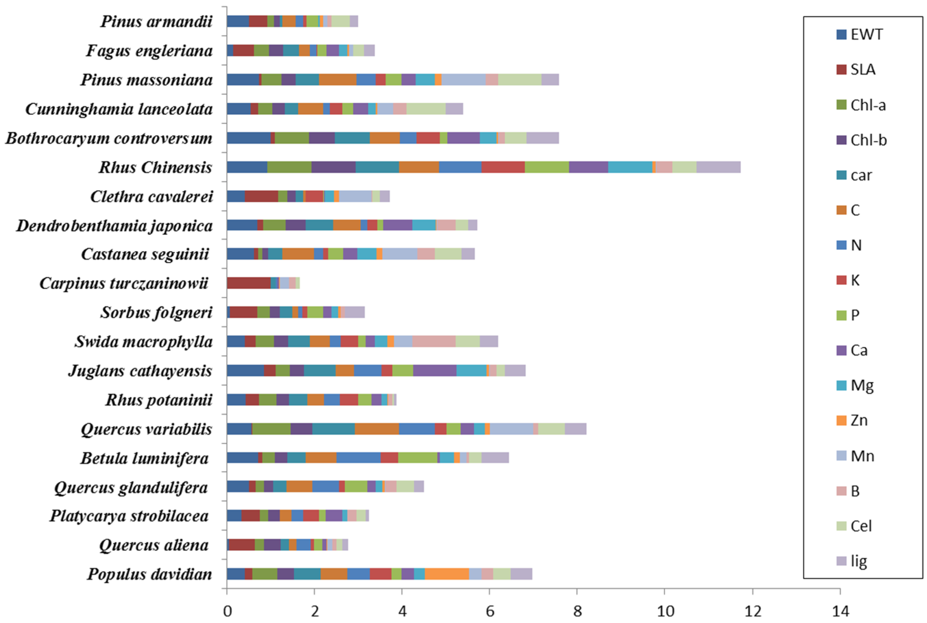
3.1. Forest Species Have Unique Biochemical Properties
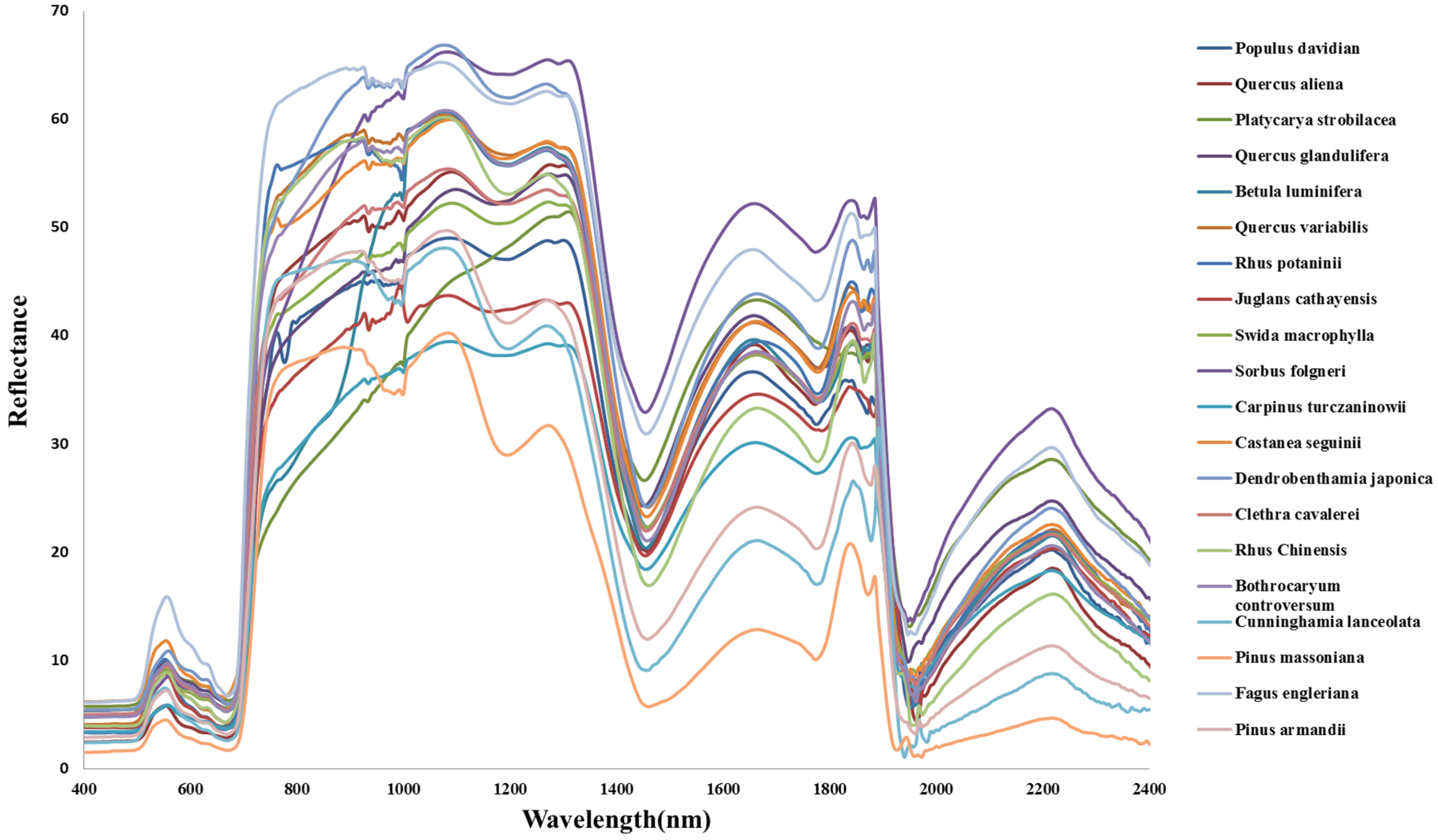
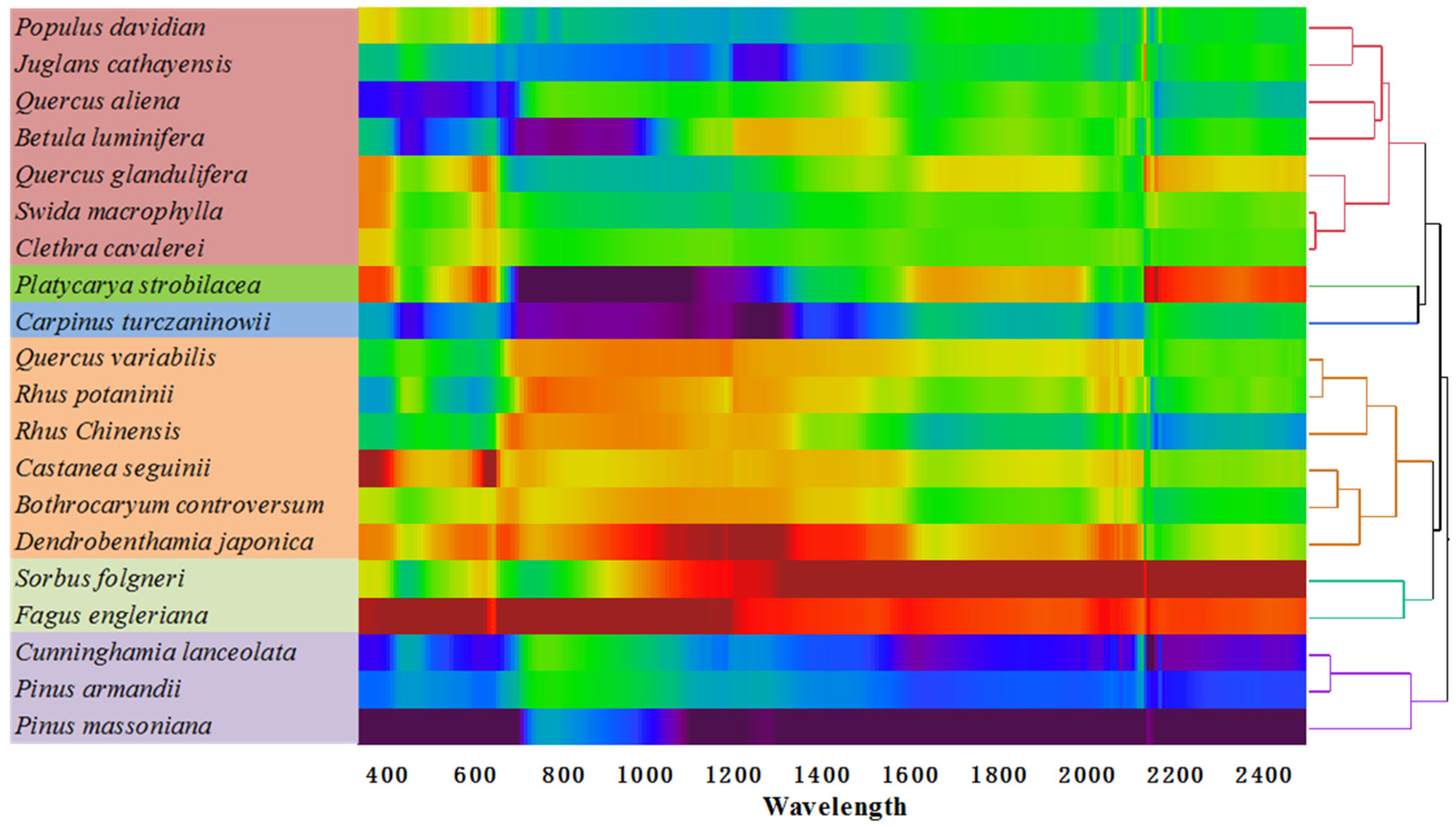
3.2. Forest Species Have Distinctive Spectral Signatures
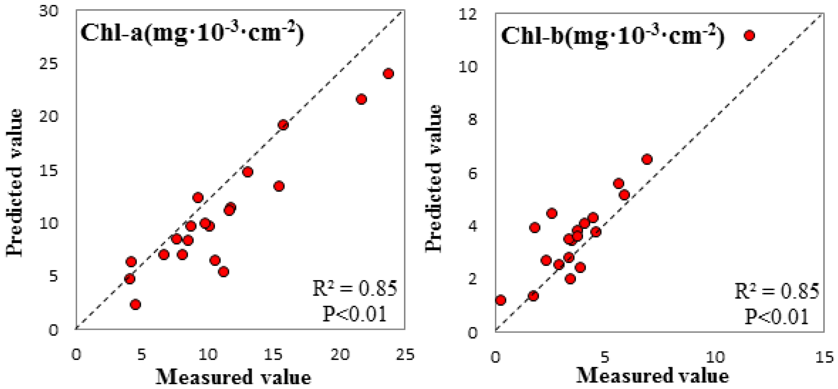
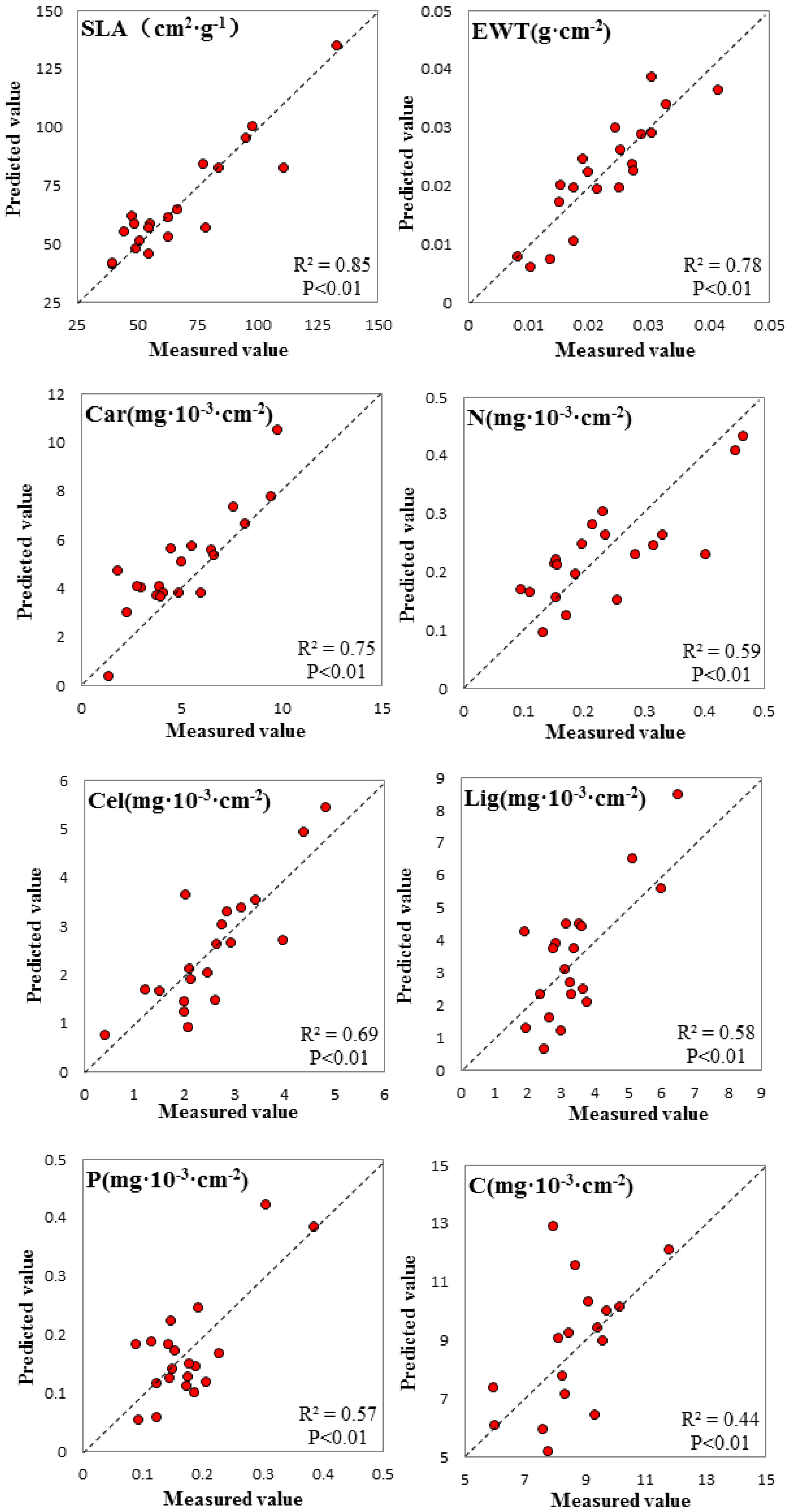
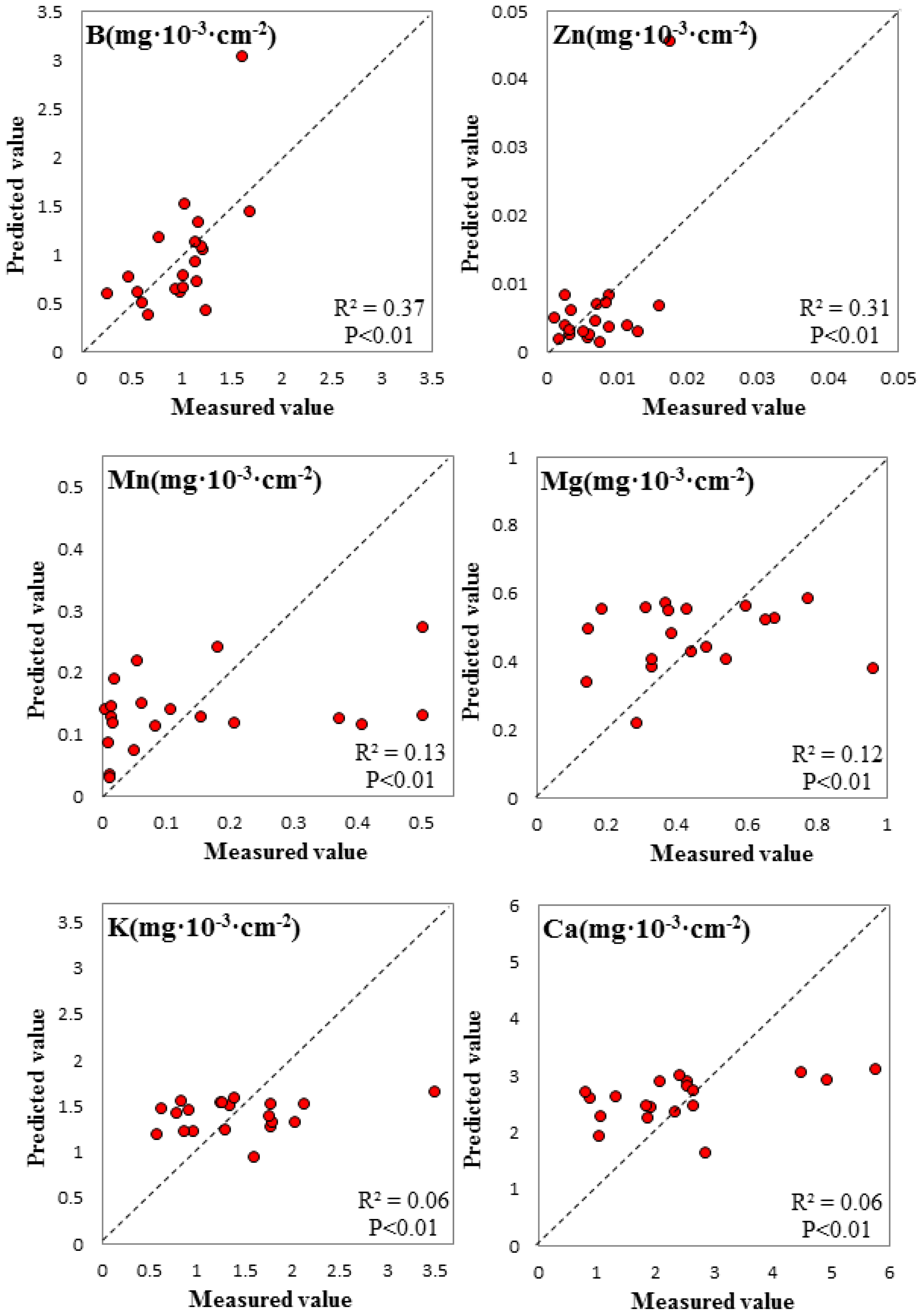
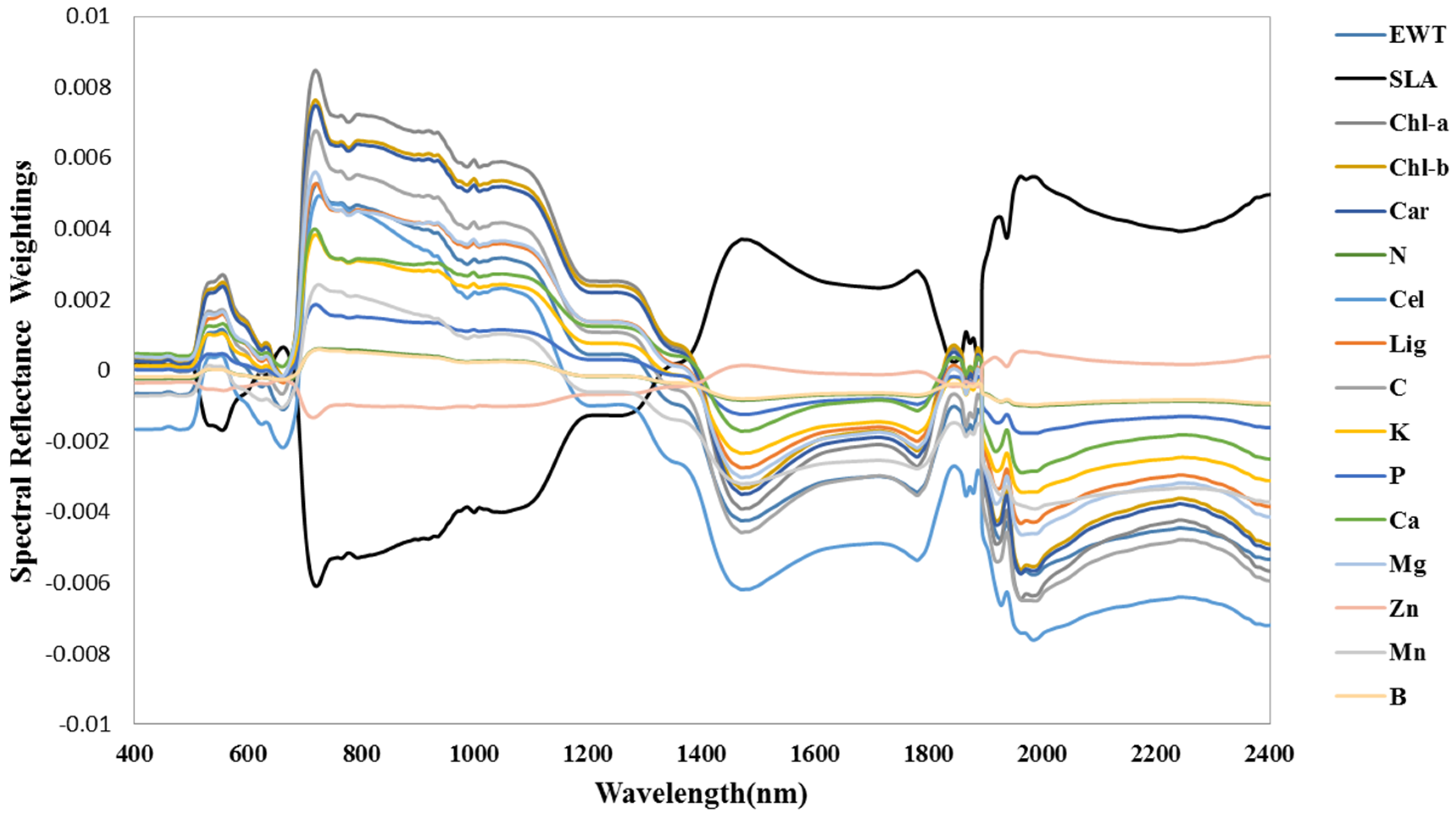
3.3. Spectral Signature Response to Biochemical Properties
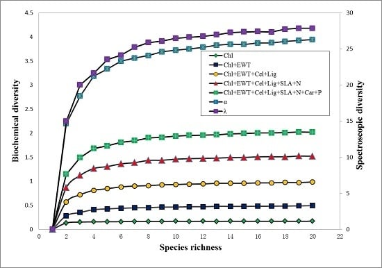
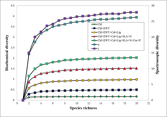
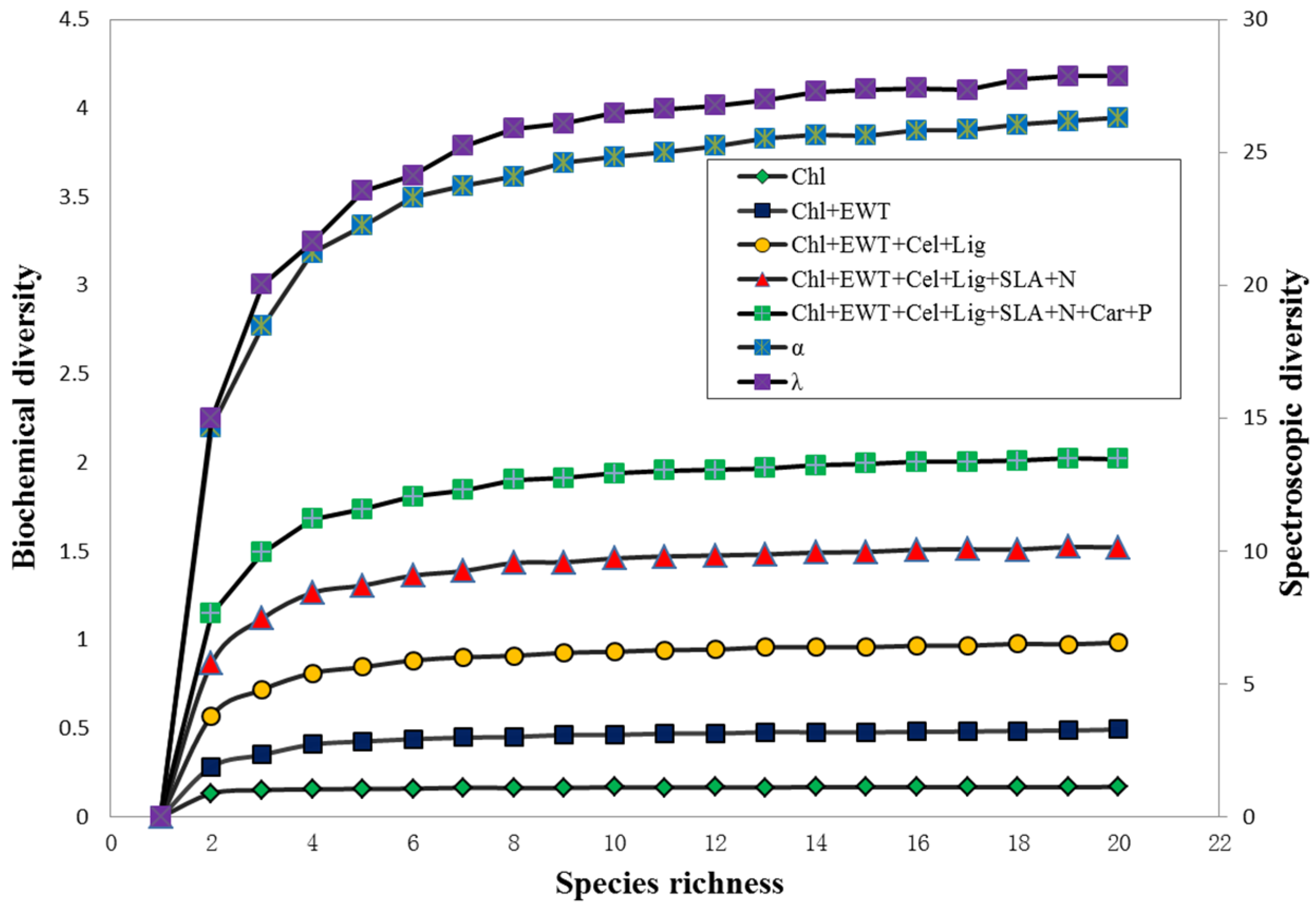
3.4. Relationships among Biochemical Diversity, Spectroscopic Diversity and Species Richness
4. Discussion
5. Conclusions
Acknowledgments
Author Contributions
Conflicts of Interest
References
- Diaz, S.; Fargione, J.; Chapin, F.S.; Tilman, D. Biodiversity loss threatens human well-being. PLoS Biol. 2006, 4, E277. [Google Scholar] [CrossRef] [PubMed]
- Harrison, P.A.; Berry, P.M.; Simpson, G.; Haslett, J.R.; Blicharska, M.; Bucur, M.; Dunford, R.; Egoh, B.; Garcia-Llorente, M.; Geamănă, N.; et al. Linkages between biodiversity attributes and ecosystem services: A systematic review. Ecosyst. Serv. 2014, 9, 191–203. [Google Scholar] [CrossRef]
- Turner, W. Sensing biodiversity. Science 2014, 346, 301–302. [Google Scholar] [CrossRef] [PubMed]
- Drakare, S.; Lennon, J.J.; Hillebrand, H. The imprint of the geographical, evolutionary and ecological context on species-area relationships. Ecol. Lett. 2006, 9, 215–227. [Google Scholar] [CrossRef] [PubMed]
- Kooistra, L.; Wamelink, W.; Schaepman-Strub, G.; Schaepman, M.; van Dobben, H.; Aduaka, U.; Batelaan, O. Assessing and predicting biodiversity in a floodplain ecosystem: Assimilation of net primary production derived from imaging spectrometer data into a dynamic vegetation model. Remote Sens. Environ. 2008, 112, 2118–2130. [Google Scholar] [CrossRef]
- Stoms, D.M.; Estes, J. A remote sensing research agenda for mapping and monitoring biodiversity. Int. J. Remote Sens. 1993, 14, 1839–1860. [Google Scholar] [CrossRef]
- Tittensor, D.P.; Micheli, F.; Nyström, M.; Worm, B. Human impacts on the species-area relationship in reef fish assemblages. Ecol. Lett. 2007, 10, 760–772. [Google Scholar] [CrossRef] [PubMed]
- Townsend, A.R.; Asner, G.P.; Cleveland, C.C. The biogeochemical heterogeneity of tropical forests. Trends Ecol. Evol. 2008, 23, 424–431. [Google Scholar] [CrossRef] [PubMed]
- Asner, G.P.; Martin, R.E. Spectral and chemical analysis of tropical forests: Scaling from leaf to canopy levels. Remote Sens. Environ. 2008, 112, 3958–3970. [Google Scholar] [CrossRef]
- Asner, G.P.; Martin, R.E. Airborne spectranomics: Mapping canopy chemical and taxonomic diversity in tropical forests. Front. Ecol. Environ. 2009, 7, 269–276. [Google Scholar] [CrossRef]
- Asner, G.P.; Martin, R.E.; Ford, A.J.; Metcalfe, D.J.; Liddell, M.J. Leaf chemical and spectral diversity in australian tropical forests. Ecol. Appl. 2009, 19, 236–253. [Google Scholar] [CrossRef] [PubMed]
- Hedin, L.O. Global organization of terrestrial plant-nutrient interactions. Proc. Natl. Acad. Sci. USA 2004, 101, 10849–10850. [Google Scholar] [CrossRef] [PubMed]
- Ustin, S.L.; Roberts, D.A.; Gamon, J.A.; Asner, G.P.; Green, R.O. Using imaging spectroscopy to study ecosystem processes and properties. Bioscience 2004, 54, 523–534. [Google Scholar] [CrossRef]
- Palmer, M.; Wohlgemuth, T.; Earls, P.; Arévalo, J.; Thompson, S. Opportunities for long-term ecological research at the tallgrass prairie preserve, Oklahoma. In Proceedings of the ILTER Regional Workshop: Cooperation in Long Term Ecological Research in Central and Eastern Europe, Budapest, Hungary, 22–25 June 1999.
- Palmer, M.W.; Earls, P.G.; Hoagland, B.W.; White, P.S.; Wohlgemuth, T. Quantitative tools for perfecting species lists. Environmetrics 2002, 13, 121–137. [Google Scholar] [CrossRef]
- Rocchini, D.; Chiarucci, A.; Loiselle, S.A. Testing the spectral variation hypothesis by using satellite multispectral images. Acta Oecol. 2004, 26, 117–120. [Google Scholar] [CrossRef]
- Oldeland, J.; Wesuls, D.; Rocchini, D.; Schmidt, M.; Jürgens, N. Does using species abundance data improve estimates of species diversity from remotely sensed spectral heterogeneity? Ecol. Indic. 2010, 10, 390–396. [Google Scholar] [CrossRef]
- Carlson, K.M.; Asner, G.P.; Hughes, R.F.; Ostertag, R.; Martin, R.E. Hyperspectral remote sensing of canopy biodiversity in hawaiian lowland rainforests. Ecosystems 2007, 10, 536–549. [Google Scholar] [CrossRef]
- Curran, P.J. Remote-sensing of foliar chemistry. Remote Sens. Environ. 1989, 30, 271–278. [Google Scholar] [CrossRef]
- Ustin, S.L.; Gitelson, A.A.; Jacquemoud, S.; Schaepman, M.; Asner, G.P.; Gamon, J.A.; Zarco-Tejada, P. Retrieval of foliar information about plant pigment systems from high resolution spectroscopy. Remote Sens. Environ. 2009, 113, S67–S77. [Google Scholar] [CrossRef] [Green Version]
- Cheng, Y.-B.; Zarco-Tejada, P.J.; Riaño, D.; Rueda, C.A.; Ustin, S.L. Estimating vegetation water content with hyperspectral data for different canopy scenarios: Relationships between AVIRIS and MODIS indexes. Remote Sens. Environ. 2006, 105, 354–366. [Google Scholar] [CrossRef]
- Gitelson, A.A.; Zur, Y.; Chivkunova, O.B.; Merzlyak, M.N. Assessing carotenoid content in plant leaves with reflectance spectroscopy. Photochem. Photobiol. 2002, 75, 272–281. [Google Scholar] [CrossRef]
- Hernández-Clemente, R.; Navarro-Cerrillo, R.M.; Zarco-Tejada, P.J. Carotenoid content estimation in a heterogeneous conifer forest using narrow-band indices and prospect + dart simulations. Remote Sens. Environ. 2012, 127, 298–315. [Google Scholar] [CrossRef]
- Serrano, L.; Penuelas, J.; Ustin, S.L. Remote sensing of nitrogen and lignin in mediterranean vegetation from AVIRIS data: Decomposing biochemical from structural signals. Remote Sens. Environ. 2002, 81, 355–364. [Google Scholar] [CrossRef]
- Serrano, L.; Ustin, S.L.; Roberts, D.A.; Gamon, J.A.; Penuelas, J. Deriving water content of chaparral vegetation from AVIRIS data. Remote Sens. Environ. 2000, 74, 570–581. [Google Scholar] [CrossRef]
- Sims, D.A.; Gamon, J.A. Relationships between leaf pigment content and spectral reflectance across a wide range of species, leaf structures and developmental stages. Remote Sens. Environ. 2002, 81, 337–354. [Google Scholar] [CrossRef]
- Suárez, L.; Zarco-Tejada, P.J.; Sepulcre-Cantó, G.; Pérez-Priego, O.; Miller, J.R.; Jiménez-Muñoz, J.C.; Sobrino, J. Assessing canopy PRI for water stress detection with diurnal airborne imagery. Remote Sens. Environ. 2008, 112, 560–575. [Google Scholar] [CrossRef]
- Wu, C.Y.; Niu, Z.; Tang, Q.; Huang, W.J. Estimating chlorophyll content from hyperspectral vegetation indices: Modeling and validation. Agric. For. Meteorol. 2008, 148, 1230–1241. [Google Scholar] [CrossRef]
- Zarco-Tejada, P.J.; Miller, J.R.; Noland, T.L.; Mohammed, G.H.; Sampson, P.H. Scaling-up and model inversion methods with narrowband optical indices for chlorophyll content estimation in closed forest canopies with hyperspectral data. IEEE Trans. Geosci. Remote Sens. 2001, 39, 1491–1507. [Google Scholar] [CrossRef]
- Qian, Y.; Zongqiang, X.; Gaoming, X.; Zhigang, C.; Jingyuan, Y. Community characteristics and population structure of dominant species of abies fargesii forests in shennongjia national nature reserve. Acta Ecol. Sin. 2008, 28, 1931–1941. [Google Scholar] [CrossRef]
- Zeng, Y.; Huang, J.X.; Wu, B.F.; Schaepman, M.E.; de Bruin, S.; Clevers, J.G.P.W. Comparison of the inversion of two canopy reflectance models for mapping forest crown closure using imaging spectroscopy. Can. J. Remote Sens. 2008, 34, 235–244. [Google Scholar]
- Zeng, Y.; Schaepman, M.E.; Wu, B.; Clevers, J.G.P.W.; Bregt, A.K. Scaling-based forest structural change detection using an inverted geometric-optical model in the three gorges region of china. Remote Sens. Environ. 2008, 112, 4261–4271. [Google Scholar] [CrossRef]
- Asner, G.; Martin, R.; Suhaili, A. Sources of canopy chemical and spectral diversity in lowland bornean forest. Ecosystems 2012, 15, 504–517. [Google Scholar] [CrossRef]
- Niinemets, Ü.; Sack, L. Structural determinants of leaf light-harvesting capacity and photosynthetic potentials. In Progress in Botany; Esser, K., Lüttge, U., Beyschlag, W., Murata, J., Eds.; Springer: Berlin, Germany; Heidelberg, Germany, 2006; Volume 67, pp. 385–419. [Google Scholar]
- Ceccato, P.; Flasse, S.; Tarantola, S.; Jacquemoud, S.; Grégoire, J.-M. Detecting vegetation leaf water content using reflectance in the optical domain. Remote Sens. Environ. 2001, 77, 22–33. [Google Scholar] [CrossRef]
- Kokaly, R.F.; Asner, G.P.; Ollinger, S.V.; Martin, M.E.; Wessman, C.A. Characterizing canopy biochemistry from imaging spectroscopy and its application to ecosystem studies. Remote Sens. Environ. 2009, 113 (Suppl. 1), S78–S91. [Google Scholar] [CrossRef]
- Lichtenthaler, H.K.; Buschmann, C. Chlorophylls and carotenoids: Measurement and characterization by UV-VIS spectroscopy. In Current Protocols in Food Analytical Chemistry; John Wiley & Sons, Inc: New York, NY, USA, 2001; pp. F4–F4.3.8. [Google Scholar]
- Savitzky, A.; Golay, M.J.E. Smoothing differentiation of data by simplified least squares procedures. Anal. Chem. 1964, 36, 1627–1639. [Google Scholar] [CrossRef]
- Ward, J.H. Hierarchical grouping to optimize an objective function. J. Am. Stat. Assoc. 1963, 58, 236–244. [Google Scholar] [CrossRef]
- Asner, G.P. 12 hyperspectral remote sensing of canopy chemistry, physiology, and biodiversity in tropical rainforests. In Hyperspectral Remote Sensing of Tropical and Sub-Tropical Forests; Taylor and Francis Group: Boca Raton, FL, USA, 2008; pp. 261–296. [Google Scholar]
- John, R.; Dalling, J.W.; Harms, K.E.; Yavitt, J.B.; Stallard, R.F.; Mirabello, M.; Hubbell, S.P.; Valencia, R.; Navarrete, H.; Vallejo, M.; et al. Soil nutrients influence spatial distributions of tropical trees species. Proc. Natl. Acad. Sci. USA 2007, 104, 864–869. [Google Scholar] [CrossRef] [PubMed]
- McGroddy, M.E.; Daufresne, T.; Hedin, L.O. Scaling of C:N:P stoichiometry in forests worldwide: Implications of terrestrial redfield-type ratios. Ecology 2004, 85, 2390–2401. [Google Scholar] [CrossRef]
- Daughtry, C.S.T.; Walthall, C.L.; Kim, M.S.; de Colstoun, E.B.; McMurtrey Iii, J.E. Estimating corn leaf chlorophyll concentration from leaf and canopy reflectance. Remote Sens. Environ. 2000, 74, 229–239. [Google Scholar] [CrossRef]
- Gamon, J.A.; Penuelas, J.; Field, C.B. A narrow-waveband spectral index that tracks diurnal changes in photosynthetic efficiency. Remote Sens. Environ. 1992, 41, 35–44. [Google Scholar] [CrossRef]
- Kim, M.S.; Daughtry, C.; Chappelle, E.; McMurtrey, J.; Walthall, C. The use of high spectral resolution bands for estimating absorbed photosynthetically active radiation (a par). In Proceedings of 6th International Symposium on Physical Measurements and Signatures in Remote Sensing, Greenbelt, MD, USA, 1 January 1994.
- Mutanga, O.; Skidmore, A.K.; van Wieren, S. Discriminating tropical grass (cenchrus ciliaris) canopies grown under different nitrogen treatments using spectroradiometry. ISPRS J. Photogramm. Remote Sens. 2003, 57, 263–272. [Google Scholar] [CrossRef]
- Roberts, D.A.; Green, R.O.; Adams, J.B. Temporal and spatial patterns in vegetation and atmospheric properties from AVIRIS. Remote Sens. Environ. 1997, 62, 223–240. [Google Scholar] [CrossRef]
- Ustin, S.L.; Roberts, D.A.; Pinzón, J.; Jacquemoud, S.; Gardner, M.; Scheer, G.; Castañeda, C.M.; Palacios-Orueta, A. Estimating canopy water content of chaparral shrubs using optical methods. Remote Sens. Environ. 1998, 65, 280–291. [Google Scholar] [CrossRef]
- Chen, J.M.; Rich, P.M.; Gower, S.T.; Norman, J.M.; Plummer, S. Leaf area index of boreal forests: Theory, techniques, and measurements. J. Geophys. Res. Atmos. 1997, 102, 29429–29443. [Google Scholar] [CrossRef]
- Kuusk, A. A two-layer canopy reflectance model. J. Quant. Spectrosc. Radiat. Transf. 2001, 71, 1–9. [Google Scholar] [CrossRef]
- Kuusk, A.; Nilson, T. A directional multispectral forest reflectance model. Remote Sens. Environ. 2000, 72, 244–252. [Google Scholar] [CrossRef]
- Malenovský, Z.; Homolová, L.; Zurita-Milla, R.; Lukeš, P.; Kaplan, V.; Hanuš, J.; Gastellu-Etchegorry, J.-P.; Schaepman, M.E. Retrieval of spruce leaf chlorophyll content from airborne image data using continuum removal and radiative transfer. Remote Sens. Environ. 2013, 131, 85–102. [Google Scholar] [CrossRef]
- Dubayah, R.O.; Sheldon, S.L.; Clark, D.B.; Hofton, M.A.; Blair, J.B.; Hurtt, G.C.; Chazdon, R.L. Estimation of tropical forest height and biomass dynamics using LiDAR remote sensing at La Selva, Costa Rica. J. Geophys. Res. Biogeosci. 2010, 115. [Google Scholar] [CrossRef]
- Lefsky, M.A.; Hudak, A.T.; Cohen, W.B.; Acker, S.A. Geographic variability in LiDAR predictions of forest stand structure in the pacific northwest. Remote Sens. Environ. 2005, 95, 532–548. [Google Scholar] [CrossRef]
- Simonson, W.D.; Allen, H.D.; Coomes, D.A. Use of an airborne LiDAR system to model plant species composition and diversity of mediterranean oak forests. Conserv. Biol. 2012, 26, 840–850. [Google Scholar] [CrossRef] [PubMed]
- Morsdorf, F.; Kotz, B.; Meier, E.; Itten, K.I.; Allgower, B. Estimation of lai and fractional cover from small footprint airborne laser scanning data based on gap fraction. Remote Sens. Environ. 2006, 104, 50–61. [Google Scholar] [CrossRef]
- Morsdorf, F.; Nichol, C.; Malthus, T.; Woodhouse, I.H. Assessing forest structural and physiological information content of multi-spectral LiDAR waveforms by radiative transfer modelling. Remote Sens. Environ. 2009, 113, 2152–2163. [Google Scholar] [CrossRef] [Green Version]
- Zhao, D.; Pang, Y.; Li, Z.Y.; Liu, L.J. Isolating individual trees in a closed coniferous forest using small footprint LiDAR data. Int. J. Remote Sens. 2014, 35, 7199–7218. [Google Scholar] [CrossRef]
- Disney, M.I.; Lewis, P.E.; Bouvet, M.; Prieto-Blanco, A.; Hancock, S. Quantifying surface reflectivity for spaceborne LiDAR via two independent methods. IEEE Trans. Geosci. Remote Sens. 2009, 47, 3262–3271. [Google Scholar] [CrossRef]
- Gastellu-Etchegorry, J.-P.; Yin, T.; Lauret, N.; Cajgfinger, T.; Gregoire, T.; Grau, E.; Feret, J.-B.; Lopes, M.; Guilleux, J.; Dedieu, G.; et al. Discrete anisotropic radiative transfer (Dart 5) for modeling airborne and satellite spectroradiometer and LiDAR acquisitions of natural and urban landscapes. Remote Sens. 2015, 7, 1667–1701. [Google Scholar] [CrossRef] [Green Version]
- Dalponte, M.; Bruzzone, L.; Vescovo, L.; Gianelle, D. The role of spectral resolution and classifier complexity in the analysis of hyperspectral images of forest areas. Remote Sens. Environ. 2009, 113, 2345–2355. [Google Scholar] [CrossRef]
- Féret, J.; Asner, G.P. Tree species discrimination in tropical forests using airborne imaging spectroscopy. IEEE Trans. Geosci. Remote Sens. 2013, 51, 73–84. [Google Scholar] [CrossRef]
- Naidoo, L.; Cho, M.A.; Mathieu, R.; Asner, G. Classification of savanna tree species, in the greater kruger national park region, by integrating hyperspectral and LiDAR data in a random forest data mining environment. Isprs J. Photogramm. Remote Sens. 2012, 69, 167–179. [Google Scholar] [CrossRef]
- Schneider, F.D.; Leiterer, R.; Morsdorf, F.; Gastellu-Etchegorry, J.-P.; Lauret, N.; Pfeifer, N.; Schaepman, M.E. Simulating imaging spectrometer data: 3D forest modeling based on LiDAR and in situ data. Remote Sens. Environ. 2014, 152, 235–250. [Google Scholar] [CrossRef]
- Brandtberg, T. Classifying individual tree species under leaf-off and leaf-on conditions using airborne LiDAR. ISPRS J. Photogramm. Remote Sens. 2007, 61, 325–340. [Google Scholar] [CrossRef]
- Mura, M.; McRoberts, R.E.; Chirici, G.; Marchetti, M. Estimating and mapping forest structural diversity using airborne laser scanning data. Remote Sens. Environ. 2015, 170, 133–142. [Google Scholar] [CrossRef]
- Cho, M.A.; Mathieu, R.; Asner, G.P.; Naidoo, L.; van Aardt, J.; Ramoelo, A.; Debba, P.; Wessels, K.; Main, R.; Smit, I.P.J.; et al. Mapping tree species composition in south african savannas using an integrated airborne spectral and LiDAR system. Remote Sens. Environ. 2012, 125, 214–226. [Google Scholar] [CrossRef]
- Colgan, M.S.; Baldeck, C.A.; Feret, J.B.; Asner, G.P. Mapping savanna tree species at ecosystem scales using support vector machine classification and BRDF correction on airborne hyperspectral and LiDAR data. Remote Sens. 2012, 4, 3462–3480. [Google Scholar] [CrossRef]


| Tree Species | EWT | SLA | Chl-a | Chl-b | Ca | C | N | K | P | Ca | Mg | Zn | Mn | B | Cel | Lig |
|---|---|---|---|---|---|---|---|---|---|---|---|---|---|---|---|---|
| Populus davidiana | 0.019 | 54.66 | 14.82 | 4.57 | 6.4 | 9.28 | 0.28 | 2.01 | 0.14 | 2.32 | 0.44 | 0.0457 | 0.152 | 1.06 | 2.68 | 4.54 |
| Quercus aliena | 0.0075 | 94.71 | 7.07 | 4.43 | 2.96 | 5.24 | 0.21 | 0.77 | 0.13 | 1.29 | 0.14 | 0.0023 | 0.061 | 0.62 | 1.46 | 1.65 |
| Platycarya strobilacea | 0.017 | 77.21 | 6.48 | 3.37 | 1.3 | 6.1 | 0.19 | 1.59 | 0.11 | 2.83 | 0.28 | 0.0015 | 0.009 | 0.94 | 1.7 | 1.33 |
| Quercus glandulifera | 0.022 | 54.41 | 6.62 | 2.57 | 3.86 | 9.12 | 0.31 | 0.95 | 0.25 | 1.85 | 0.33 | 0.0039 | 0.008 | 1.09 | 2.65 | 2.36 |
| Betula luminifera | 0.029 | 48.82 | 8.4 | 3.48 | 4.92 | 10.17 | 0.46 | 1.76 | 0.39 | 1.03 | 0.53 | 0.0071 | 0.082 | 0.52 | 2.15 | 5.61 |
| Quercus variabilis | 0.025 | 39.20 | 21.68 | 5.87 | 9.44 | 12.93 | 0.40 | 1.34 | 0.17 | 2.51 | 0.43 | 0.0064 | 0.499 | 0.66 | 3.67 | 4.53 |
| Rhus potaninii | 0.020 | 66.21 | 11.48 | 3.32 | 4.83 | 7.18 | 0.23 | 1.76 | 0.17 | 2.05 | 0.31 | 0.002 | 0.004 | 0.63 | 0.95 | 1.26 |
| Juglans cathayensis | 0.034 | 62.17 | 9.81 | 3.70 | 7.56 | 7.41 | 0.33 | 1.28 | 0.23 | 6.31 | 0.96 | 0.004 | 0.013 | 0.78 | 1.71 | 4.48 |
| Swida macrophylla | 0.019 | 62.21 | 11.25 | 4.02 | 5.47 | 7.83 | 0.18 | 1.78 | 0.12 | 1.89 | 0.48 | 0.0085 | 0.206 | 3.04 | 3.32 | 3.96 |
| Sorbus folgneri | 0.0081 | 97.71 | 8.60 | 2.87 | 3.68 | 4.99 | 0.13 | 0.85 | 0.19 | 1.82 | 0.32 | 0.0040 | 0.009 | 0.61 | 0.78 | 4.31 |
| Carpinus turczaninowii | 0.0063 | 132.46 | 2.42 | 0.23 | 2.19 | 3.66 | 0.11 | 0.56 | 0.06 | 1.01 | 0.14 | 0.0027 | 0.106 | 0.79 | 1.25 | 0.69 |
| Castanea seguinii | 0.026 | 47.31 | 4.86 | 1.69 | 4.02 | 10.34 | 0.17 | 0.90 | 0.19 | 2.51 | 0.67 | 0.0069 | 0.404 | 1.45 | 3.57 | 3.13 |
| Dendrobenthamia japonica | 0.029 | 50.24 | 13.54 | 5.57 | 6.57 | 9.45 | 0.15 | 1.23 | 0.10 | 4.47 | 0.77 | 0.0026 | 0.014 | 1.53 | 2.06 | 2.37 |
| Clethra cavalerei | 0.020 | 110.2 | 7.08 | 2.27 | 2.72 | 4.21 | 0.09 | 1.75 | 0.056 | 0.87 | 0.38 | 0.0074 | 0.37 | 0.44 | 1.51 | 2.53 |
| Rhus chinensis | 0.037 | 38.97 | 24.12 | 11.55 | 9.75 | 12.14 | 0.45 | 3.48 | 0.42 | 5.75 | 1.33 | 0.0051 | 0.016 | 1.35 | 3.40 | 8.52 |
| Bothrocaryum controversum | 0.039 | 48.09 | 19.34 | 6.86 | 8.11 | 10.03 | 0.23 | 2.11 | 0.12 | 4.9 | 0.59 | 0.0031 | 0.013 | 0.74 | 3.06 | 6.55 |
| Cunninghamia lanceolata | 0.024 | 54.12 | 9.79 | 3.33 | 3.88 | 9.02 | 0.15 | 1.37 | 0.15 | 2.62 | 0.36 | 0.0031 | 0.18 | 1.19 | 4.97 | 3.78 |
| Pinus massoniana | 0.030 | 44.12 | 12.47 | 3.85 | 5.89 | 11.59 | 0.25 | 1.24 | 0.19 | 2.63 | 0.65 | 0.0085 | 0.499 | 1.13 | 5.46 | 3.76 |
| Fagus engleriana | 0.011 | 83.35 | 10.08 | 3.72 | 4.44 | 5.97 | 0.15 | 0.61 | 0.13 | 2.4 | 0.37 | 0.0033 | 0.047 | 0.39 | 1.93 | 2.72 |
| Pinus armandii | 0.023 | 78.12 | 5.50 | 1.79 | 1.79 | 6.46 | 0.15 | 0.82 | 0.15 | 0.79 | 0.18 | 0.0047 | 0.053 | 0.67 | 2.73 | 2.13 |
© 2016 by the authors; licensee MDPI, Basel, Switzerland. This article is an open access article distributed under the terms and conditions of the Creative Commons by Attribution (CC-BY) license (http://creativecommons.org/licenses/by/4.0/).
Share and Cite
Zhao, Y.; Zeng, Y.; Zhao, D.; Wu, B.; Zhao, Q. The Optimal Leaf Biochemical Selection for Mapping Species Diversity Based on Imaging Spectroscopy. Remote Sens. 2016, 8, 216. https://doi.org/10.3390/rs8030216
Zhao Y, Zeng Y, Zhao D, Wu B, Zhao Q. The Optimal Leaf Biochemical Selection for Mapping Species Diversity Based on Imaging Spectroscopy. Remote Sensing. 2016; 8(3):216. https://doi.org/10.3390/rs8030216
Chicago/Turabian StyleZhao, Yujin, Yuan Zeng, Dan Zhao, Bingfang Wu, and Qianjun Zhao. 2016. "The Optimal Leaf Biochemical Selection for Mapping Species Diversity Based on Imaging Spectroscopy" Remote Sensing 8, no. 3: 216. https://doi.org/10.3390/rs8030216