Article

A New Method for the Estimation of Broadband Apparent Albedo Using Hyperspectral Airborne Hemispherical Directional Reflectance Factor Values

by
Javier F. Calleja
1,*,
Carmen Recondo
2,3,
Juanjo Peón
2,
Susana Fernández
4,
Fernando De la Cruz
5 and
José González-Piqueras
6
1
Departamento de Física, Universidad de Oviedo, Calvo Sotelo s/n, 33007 Oviedo, Spain
2
Área de Ingeniería Cartográfica, Geodésica y Fotogrametría, Departamento de Explotación y Prospección de Minas, Universidad de Oviedo, Gonzalo Gutiérrez Quirós s/n, 33600 Mieres, Spain
3
Instituto de Recursos Naturales y Ordenación del Territorio (INDUROT), Universidad de Oviedo, Gonzalo Gutiérrez Quirós s/n, 33600 Mieres, Spain
4
Departamento de Geología, Universidad de Oviedo, Jesús Arias de Velasco s/n, 33005 Oviedo, Spain
5
Instituto Técnico Agronómico Provincial (ITAP), Polígono Industrial Campollano, Avda.2ª, No. 42B, 02007 Albacete, Spain
6
Instituto Desarrollo Regional (IDR), Grupo Teledetección y SIG, Universidad Castilla La Mancha, Campus Universitario s/n, 02071 Albacete, Spain
*
Author to whom correspondence should be addressed.
Remote Sens. 2016, 8(3), 183; https://doi.org/10.3390/rs8030183
Submission received: 15 July 2015 / Revised: 4 February 2016 / Accepted: 14 February 2016 / Published: 25 February 2016
(This article belongs to the Special Issue Field Spectroscopy and Radiometry)

Abstract

:
The broadband albedo values retrieved from satellite sensors are usually compared directly to ground measurements. Some authors have noted the necessity of high spatial resolution albedo estimates to fill the gap between ground measurements and satellite retrievals. In this respect, hyperspectral airborne data with high spatial resolution is a powerful tool. Here, a new operational method for the calculation of airborne broadband apparent albedo over the spectral range of 350–2500 nm is presented. This new method uses the Hemispherical Directional Reflectance Factor (HDRF) as a proxy for the narrowband albedo, assuming a Lambertian approximation. The broadband apparent albedo obtained is compared to that estimated using theapparent albedo equation devised for the Moderate Resolution Imaging Spectroradiometer (MODIS). Airborne data were collected using the Airborne Hyperspectral Scanner (AHS). Field data were acquired at three sites: a camelina field, a green grass field, and a vineyard.  The HDRF can be used to approximate the narrowband albedo for all View Zenith Angle (VZA) values for flights parallel to the solar principal plane (SPP); for flights orthogonal to the SPP, discrepancies are observed when the VZA approaches −45°. Root Mean Square Error (RMSE) values in the range 0.009–0.018 were obtained using the new method, improving upon previous results over the same area (RMSEs of 0.01–0.03). The relative error in the albedo estimation using the new method is 12% for −36.2° < VZA < 40.8° in the case of flights parallel to the SPP and less than 15% for −13° < VZA < 45° and 45% for VZA = −45° for flights orthogonal to the SPP. The good performance of the new method lies in the use of the at-surface solar irradiance and the proposed integration method.

Graphical Abstract

1. Introduction

Land surface albedo is a key parameter in the Earth’s surface energy balance and climate studies. It is an input required in the surface energy balance (SEB) and evapotranspiration (ET) models used for agricultural and water resource management, as well as in the global climate models (GCM) and weather forecasting models [1,2]. However, different models compute surface albedo differently and yield albedo values with a large spread [3]. This spread is a major source of uncertainty in radiative transfer calculations [4,5], current climatic modeling [6], and ET estimations [7].
The different SEB models provide estimates of instantaneous surface fluxes by solving the energy balance equation for net radiation (Rn), soil heat flux (G), sensible heat (H), and latent heat (LE). They have in common the estimation of net radiation [8,9] but use different approaches to estimate H and LE. Some models use the stability functions for separating canopy and soil transpiration [1] by means of internal calibration of extreme temperatures within the scene [2,10]; other models avoid the stability theory functions by using the evaporative fraction [11]. In all these SEB models, net radiation is computed from the albedo, the incoming shortwave radiation and the incoming longwave radiation [8]. The typical uncertainty in the net radiation estimate in agricultural areas using remote sensing data is between 5% and 15%, which corresponds to an error between 15% and 30% in LE and H fluxes [9,12]. Despite this sensitivity, the only research analyzing the impact of albedo accuracy has been performed with respect to the evaporative fraction-based models [7]. This research has found relative errors for H and LE ranging from 23% to 39% and 6% to 18%, respectively, for the same albedo range presented in this work. This analysis is out of the scope of this work, but the discussion of the operative approaches used to calculate the broadband albedo and the influence of the angular observations should be conducted to account for its impact on the cited models.
Currently, hyperspectral and high-resolution imagery is complementing operational multi-spectral and low to medium spatial resolution images, such as those produced by Landsat (30 m, six optical bands), MODIS (500 m, seven bands), and the future Sentinel-3 (500 m, 11 bands), in precision agriculture, modern studies of SEB and ET estimation, and mapping or other local studies focusing on water management and nutrient supply. Therefore, it is necessary to obtain new operational methods for the albedo calculation, similar to those proposed by Tasumi et al. [13], but using specific coefficients for the numerous bands of these images.
The algorithms for estimating surface broadband albedo can be classified in four categories [14]: Narrow-to-Broadband conversions, Bidirectional Reflectance Distribution Function (BRDF) angular modeling, Direct-Estimation algorithms, and algorithms specially developed for geostationary satellites. Narrow-to-Broadband albedo algorithms assume that the land is Lambertian. The broadband albedo can then be estimated from linear combinations of narrowband albedo with different coefficients. Liang [15] proposed a formula to obtain shortwave (300 to 3000 nm) surface broadband apparent albedo from narrowband albedo for MODIS:
ρ   =   0.160   ρ 1 +   0.291 ρ 2 +   0.243 ρ 3 +   0.116 ρ 4 +   0.112 ρ 5 +   0.081 ρ 7 0.0015
where ρ is the broadband albedo and ρi is the spectral albedo of the MODIS band i.
Equation (1) has been applied to the Airborne Hyperspectral Scanner AHS in spite of the spectral mismatch between MODIS bands and AHS channels. When applied to AHS, Equation (1) becomes [7,16]
ρ   =   0.160   ρ 8 +   0.291 ρ 15 +   0.243 ρ 2 +   0.116 ρ 5 +   0.112 ρ 20 +   0.081 ρ 35 0.0015
where ρ is the broadband albedo and ρ¡ is the narrowband albedo of channel i. The coefficients in Equation (1) are calculated through extensive radiative transfer modeling using measured reflectance spectra and simulated solar radiative fluxes. The main advantage of this approach is that broadband albedo can be estimated from a single observation. Some authors calculate the broadband albedo by integrating the at-surface reflectance across the shortwave spectrum [13]. The coefficients in this case are calculated using a simulated at-surface solar irradiance. These methods have been proven to be very useful. The method proposed by Tasumi et al. [13] is currently one of the most used, and it has been implemented in the operational applications of the METRIC (Mapping Evapotranspiration with Internalized Calibration) model [2]. In the BRDF modeling approach, the surface is not assumed to be Lambertian; thus, it is necessary to build a BRDF model that describes the surface reflectance with different solar and view angles. Narrowband albedo is calculated by integrating the BRDF over the solar and view hemispheres. The broadband albedo is then calculated as a linear combination of the narrowband albedo with different coefficients. The linear combination is found using the same procedure as in the Narrow-to-Broadband albedo algorithm. This is the procedure used to generate the MODIS BRDF/Albedo products [17] using multi-angular MODIS data collected during a 16-day observation cycle. The broadband inherent albedo is calculated using the linear combination of narrowband albedo proposed in Liang et al. [18]. This algorithm requires multiangular data; thus, it cannot be applied to a single observation. The Direct-Estimation algorithm is based on calculating the broadband albedo from the apparent reflectance without the need for atmospheric correction. The broadband albedo is calculated as a linear combination of apparent reflectance at certain specific bands. This procedure was applied to MODIS [18] and has recently been applied to the Airborne Visible Infrared Imaging Spectrometer (AVIRIS) [19]. This algorithm can be applied to a single observation. It requires extensive radiative transfer modeling to simulate the surface albedo and the surface apparent reflectance. Broadband albedo estimates from geostationary satellites are quite different from the previous methods, but they also require BRDF modeling and Narrow-to-Broadband conversion.
Although the Lambertian approximation has been extensively used [15,20], real surfaces are non-Lambertian and their directional reflectance depends on illumination and viewing directions. The non-Lambertian behavior of vegetated surfaces is well documented and the anisotropy in reflectance has been documented from field measurements [21,22,23] and remote sensing data [22,23,24,25]. The anisotropy in reflectance is mainly caused by canopy structure and architectural properties. In this respect, BRDF in semiempirical models is expressed as a linear combination of three contributions [26]: a constant corresponding to isotropic reflectance, the volume scattering from canopy and the geometric-optical surface scattering from 3D objects casting shadows. The maximum values of reflectance are obtained for the highest VZA, where only the upper and most illuminated top of the canopies are seen by the sensor. This is the so-called gap effect. The gap effect is more important for dense and high canopies [22,23,24] and is observed along any viewing direction. The combination of the gap effect and the effect of shadows is responsible for the anisotropy in the reflectance. The influence of shadows depends on the viewing direction and on the solar zenith angle (SZA). When reflectance is measured along the plane orthogonal to the solar principal plane, the shadow pattern is symmetrical with respect to the nadir view, yielding a symmetrical reflectance with respect to the nadir-viewing direction [22]. When reflectance is measured along the solar principal plane, shaded areas are detected from the forward scattering direction, producing a decrease in the radiance received by the sensor. However, shaded areas disappear for areas observed from the backscattering direction. This produces a high anisotropy in reflectance measured along the solar principal plane [21,22,23,24]. Regarding the SZA, increasing values of the SZA cause an increase of shaded areas with the corresponding decrease in reflectance [22,24]. Furthermore, the impact of shadows depends on the instantaneous field of view (IFOV) of the sensor [24], which determines the size of the ground sample distance (the size of a pixel of a remote sensing image). A larger ground sample distance gives rise to a mixture of signal from illuminated and shaded areas and thus diminishes the magnitude of reflectance anisotropy [25]. On the other hand, smaller ground sample distance increases the contribution of shadows to the reflectance anisotropy [25]. In addition to this, the reflectance anisotropy depends on the wavelength of the radiation. For instance, geometric-optical effects have less influence on the NIR due to increased multiple scattering [22,23,24]. In this paper, we use HDRF as a proxy for the narrowband albedo, assuming a Lambertian approximation. The approximation is expected to be valid when the HDRF depends only slightly on the viewing direction and the SZA. We carry out a study of the dependence of the airborne HDRF on the viewing direction and on the SZA to establish the limiting conditions of the approximation. Then, we perform a statistical analysis of the error in the broadband albedo obtained using the HDRF.
Regarding validation of albedo data retrieved from remote sensing sensors, medium/coarse resolution satellite-retrieved albedo data are usually compared directly to ground measurements. Some authors have noted the necessity of high spatial resolution albedo estimates to fill the gap between ground measurements and satellite retrievals [19,27]. Some improvements have already been introduced into the validation of Landsat and MODIS albedo using airborne albedo retrievals as an intermediate step between ground and satellite data [28]. However, an easy-to-use algorithm to estimate the apparent albedo from airborne hyperspectral data is still lacking. In this work, we intend to fill this gap. From our perspective, to say that a method is easy to use means that the method can be applied to a single observation and does not require intensive radiative modeling. The Narrow-to-Broadband and the Direct-Estimation algorithms require extensive radiative modeling and rely on simulated solar fluxes. The BRDF modeling approach demands multiangular observations.
The objective of this work is to develop a new procedure to calculate the broadband apparent albedo from airborne data using a single observation (a single image) and using the Hemispherical Directional Reflectance Factor (HDRF) as a proxy for the narrowband albedo. It is also our purpose to determine the experimental conditions under which this procedure can be applied because of the non-Lambertian nature of real surfaces. We are interested in the broadband apparent albedo because this is the product that can be directly compared to field data [13,18]. We intend to use the HDRF because it is the product that results from the atmospheric correction when using the Atmospheric and Topographic Correction software (ATCOR4) [29,30]. We calculate the broadband apparent albedo as a linear combination of the spectral HDRF. The coefficients of the linear combination are calculated by integrating the spectral HDRF using measured downwelling reflected irradiance over a white reference panel. This new procedure is then compared to the broadband apparent albedo estimated using Equation (2). This comparison is carried out because, as previously noted, Equation (2) has been used despite the spectral mismatch between the AHS and MODIS sensors.
The fact that the new procedure to estimate the broadband albedo proposed in this work can be applied to a single observation implies that no BRDF modeling is needed.

2. Materials and Methods

In this work we investigate the dependence of the HDRF on the viewing direction and on the SZA to check the validity of the approximation consisting of using the HDRF as a proxy for the narrowband albedo. We then proceed with the narrow to broadband albedo conversion using the HDRF as a proxy for the narrowband albedo. The narrow to broadband conversion is performed by applying two algorithms. The first algorithm is a new method proposed by the authors. The second algorithm is based on the equation proposed for MODIS broadband apparent albedo, which has been applied to AHS by other authors (Equation (2)) [7,16]. We then proceed with the validation, the estimation of the errors and the discussion. Figure 1 shows a flow chart of the procedure followed in this paper. Because we use an approximation that consists of considering HDRF to be independent of the viewing direction, the validation is carried out as a function of the viewing direction to check the validity of this approximation.

2.1. Theory

The broadband apparent albedo ρ A (at an incident solar zenith angle θ and for a wavelength range Λ) is defined as follows [18]:
ρ A ( θ ,   Λ ) = F u F d = λ l λ u ρ ( θ , λ ) F d ( θ , λ ) d λ λ l λ u F d ( θ , λ ) d λ
where Fu is the broadband upwelling energy flux reflected by a unit surface into the whole hemisphere and Fd is the broadband downwelling incident energy flux for a hemispherical angular extent (at-surface solar irradiance). Fu( θ , λ)= ρ ( θ , λ ) F d ( θ , λ ) and Fd( θ , λ) are the corresponding spectral energy fluxes, and ρ( θ , λ) is the spectral albedo (narrowband albedo). λu and λl are the upper and lower limits, respectively, of the interval Λ of the electromagnetic spectrum over which the broadband albedo is calculated.
Let us assume ρ(θ,λ) is a continuous piecewise function that attains a constant value over an interval equal to the bandwidth of each of the channels or bands of the sensor. Then, Equation (3) can be written as follows:
ρ A = F u F d = c = 1 c = N ρ c λ l c λ u c F d ( θ , λ ) d λ λ l λ u F d ( θ , λ ) d λ = c = 1 c = N ρ c ω c
where N is the number of bands or channels of the sensor, λuc and λlc are the upper and lower wavelengths of the c channel, ωc is the narrowband albedo of the c channel, and 𝜔c is the relative weight of channel c in the whole spectral range considered. To calculate the broadband albedo, we need to know the at-surface solar irradiance, the upper and lower wavelengths of each channel of the sensor, and the narrowband albedo. The at-surface solar irradiance can be measured using a spectroradiometer, and λuc and λlc can be estimated from the spectral response functions of the sensor. The main problem is the estimation of the narrowband albedo. For the sake of clarity in the equations below, we omit the dependence on λ, and it is understood that all the physical quantities are spectral quantities.
The Hemispherical Directional Reflectance Factor (HDRF) is defined as follows [30,31]:
H D R F = π 0 2 π 0 π / 2 f r ( θ i , ϕ i , θ r , ϕ r )   L i c o s θ i s i n θ i d θ i d ϕ i 0 2 π 0 π / 2 L i c o s θ i s i n θ i d θ i d ϕ i
where fri, ϕi, θr, ϕr) is the BRDF (Bidirectional Reflectance Distribution Function), Li (θi, ϕi) is the incident radiance, θi and ϕi are the angles defining the incident radiation direction (illumination direction), and θr and ϕr give the direction of the reflected radiation (the viewing direction).
On the other hand, the spectral albedo is the so-called BiHemispherical Reflectance (BHR), defined as follows [30,31]:
ρ c = B H R = 0 2 π 0 π / 2 0 2 π 0 π / 2 f r c o s θ r s i n θ r d θ r d ϕ r L i c o s θ i s i n θ i d θ i d ϕ i 0 2 π 0 π / 2 L i c o s θ i s i n θ i d θ i d ϕ i
It is clear from Equations (5) and (6) that the spectral albedo is the integration of the HDRF over the viewing hemisphere. Both physical quantities are identical for a uniform Lambertian surface, as we show below. According to Nicodemus et al. [32] a Lambertian surface is one for which the reflected radiance is isotropic, with the same value for all directions (θr, ϕr) regardless of how it is irradiated. This is possible only when fr = fr,d is a constant [32]. In what follows, the subscript d is used when referring to a Lambertian surface, so HDRFd, ρcd, BHRd, and fr,d denote the HDRF, ρc, BHR, and BRDF of a Lambertian surface. Therefore, for a Lambertian surface, Equation (5) can be written as follows:
H D R F d = π 0 2 π 0 π 2 f r , d ( θ i , ϕ i , θ r , ϕ r )   L i c o s θ i s i n θ i d θ i d ϕ i 0 2 π 0 π 2 L i c o s θ i s i n θ i d θ i d ϕ i =   π f r , d 0 2 π 0 π 2 L i c o s θ i s i n θ i d θ i d ϕ i 0 2 π 0 π 2 L i c o s θ i s i n θ i d θ i d ϕ i = π f r , d
The BiHemispherical Reflectance for a Lambertian surface is:
ρ c d = B H R d = 0 2 π 0 π / 2 0 2 π 0 π / 2 f r , d c o s θ r s i n θ r d θ r d ϕ r L i c o s θ i s i n θ i d θ i d ϕ i 0 2 π 0 π / 2 L i c o s θ i s i n θ i d θ i d ϕ i =   f r , d 0 2 π 0 π 2 c o s θ r s i n θ r d θ r d ϕ r L i c o s θ i s i n θ i d θ i d ϕ i 0 2 π 0 π / 2 L i c o s θ i s i n θ i d θ i d ϕ i
Because the incident radiance L i does not depend on ( θ r ,   ϕ r ) , Equation (8) becomes:
ρ c d = B H R d = f r , d 0 2 π 0 π / 2 c o s θ r s i n θ r d θ r d ϕ r 0 2 π 0 π / 2 L i c o s θ i s i n θ i d θ i d ϕ i 0 2 π 0 π / 2 L i c o s θ i s i n θ i d θ i d ϕ i =   π f r , d
From Equations (7) and (9) we conclude that for a Lambertian surface the Hemispherical Directional Reflectance Factor and the BiHemispherical Reflectance (spectral albedo) are identical, HDRFd = BHRd. This result was also discussed in Nicodemus et al. [32] and has been used to simplify the equations of radiative transfer models when applied to a uniform Lambertian surface [33]. To calculate the spectral albedo, the BRDF must be known. This is a difficult task that requires the measurement of the incident and reflected energy fluxes in several directions. In this work we use the HDRF as a proxy for the narrowband (spectral) albedo, so the broadband apparent albedo can be calculated as follows:
ρ A = F u F d = c = 1 c = N ρ c ω c = c = 1 c = N   ( H D R F ) c   ω c
where HDRF is the Hemispherical Directional Reflectance Factor of band or channel c and ωc is the relative weight of band or channel c.

2.2. Study Area

The study area is the well-known Barrax site, located in the La Mancha region of southern Spain, 20 km west of Albacete. Because the area comprises large homogeneous land cover units and because the terrain is flat, it is a suitable test site for remote sensing applications. Approximately 65% of the area is dry land and 35% is irrigated and cultivated with different crops. Field measurements were restricted to the Las Tiesas Experimental Farm (39°3′33″N, 2°6′5″W, elevation ca. 700 m above sea level), which includes various land use types such as bare soil, vineyard, maize, barley, wheat, poppy, sunflower, walnut and pistachio orchards, forest nursery, and camelina. The climate is Mediterranean, with a low average annual rainfall (400 mm), which is mainly concentrated in spring and autumn. During the summer, daytime temperatures above 40 °C are frequent.

2.3. Field Data

Several experiments were conducted over the Las Tiesas Experimental Farm during the Regional Experiments For Land-atmosphere EXchanges (REFLEX) [34]. In this paper, we focus on the radiometric measurements in the solar range. Nadir reflectance measurements from 350 to 2500 nm, with a resolution of 1 nm, were performed using an Analytical Spectral Devices (ASD) FieldSpec 3 instrument. On 25 July 2012, measurements were taken consecutively over several targets—poppy, bare soil, stubble, black fabric, green grass, hay bales, and water—starting at 8:25 UTC and finishing at 11:02 UTC. On 26 July 2012, measurements were taken over stubble, black fabric, and green grass consecutively, starting at 8:30 UTC and finishing at 9:10 UTC. The measurement procedure included pointing the ASD instrument at the target and at a white reference panel. In this paper, we use ASD nadir measurements over the white reference panel to obtain the downwelling reflected irradiance from which to calculate the weighting coefficients of Equation (10). Because the white reference panel is supposed to behave as an ideal Lambertian flat surface, the reflectance spectrum obtained in the field over the white reference panel is corrected with a calibration file to ensure a 100% reflectance at all wavelengths.
Broadband albedo was measured at three sites during the campaign: a camelina field, a green grass field, and a vineyard. Broadband albedo at the camelina field was acquired with a four component CNR1 radiometer (Kipp & Zonen) at a height of 1 m above the ground. The measurements were recorded every 10 min from 7:10 UTC until 19:00 UTC on 25–26 July 2012. In the Green Grass field, a four component CNR1 radiometer (Kipp & Zonen) was used. The sensor was placed 2 m above the ground and measurements were recorded every minute from 6 UTC until 19:00 UTC on 25 July 2012 and from 6:00 UTC 12:00 UTC on 26 July 2012. In the Vineyard a CNR1 radiometer (Kipp & Zonen) was used, with the sensor at a height of 4 m above the ground, and the data were recorded every hour from 6:00 UTC until 19:00 UTC on 25–26 July 2012. At the three sites, the broadband albedo was calculated as the ratio of shortwave outgoing energy flux to shortwave incoming energy flux. In these instruments, the diameter of the circular area that contributes 99% of the measured flux is approximately 10 times the sensor height [35,36]; this guarantees that the measured albedo at the three sites is representative of the plot.
To compare the airborne albedos to the field measurements, both values must be as close in time as possible. We need to know the dependence of albedo on SZA to interpolate the field albedo values for the time of the flights. A thorough analysis of the parameterization of the albedo as a function of the SZA has already been carried out by other authors [37]. According to the original work by Dickinson for vegetation [38] and its successive variations that include all snow-free types of surfaces, different spectral ranges, and different seasons, [39] the albedo (ρ) can be parameterized as a function of the SZA as follows:
ρ ( S Z A ) = a 1 + d 1 + 2 d c o s   S Z A
where a (cos SZA at 60°) and d are two constants that can be adjusted to each type of surface (and, in the case of a, also to the spectral range and to the month or season of the year).

2.4. Airborne Data

Airborne data were collected by an Airborne Hyperspectral Scanner (AHS, Argon ST, Fairfax, VA, USA) mounted on the CASA 212–200 N/S 270 airplane, property of Spanish INTA (Instituto Nacional de Técnica Aeroespacial). Flights were performed on 25–26 July 2012 [34]. All the images were then georeferenced and the pixel size fixed depending on the altitude above the ground. The time of the flights, altitude above the ground, pixel size, and the flight line direction with respect to the solar principal plane (either parallel or orthogonal) are summarized in Table 1. The general pattern of the flight lines over the study area on 25 July is shown in Figure 2. The same pattern was followed on 26 July. Due to windy conditions, the flight on 25 July at 9:19 UTC was repeated at 9:28 UTC following the same flight line but in the opposite direction; hence, five flight lines are shown in Figure 2, but six flights are listed in Table 1.
The position of the target being observed by the sensor with respect to the solar principal plane plays a very important role in the discussion of our results. Figure 3 provides a detailed description of the parameters involved in the airborne data acquisition. The solar principal plane is defined as the plane that contains the sun, the target, and the normal to the target. Because the AHS is a whiskbroom line scanner, all the targets lie along a line perpendicular to the flight direction. In Figure 3, two targets, T1 and T2, are shown; the sensor is operating under nadir viewing conditions; and we assume that the terrain is flat. In Figure 3a,b, the solar principal plane is the XY plane and the Y-axis is the zenith direction. In Figure 3a, the Z-axis is the flight line and the X-axis is the scanning direction. In Figure 3b, the flight line is the X-axis and the scanning direction is the Z-axis. The Field of View (FOV) of the AHS is 90° (45° at each side of the zenith direction) and the Instantaneous Field of View (IFOV), the angle subtended by a single target from the sensor, is 2.5 mrad. The target has a size along the scanning direction equal to the pixel size. The View Zenith Angle (VZA) of a target is defined as the angle from the zenith to the line that joins the middle point of the target and the sensor. The viewing direction is defined by the VZA and the scanning direction. In Figure 3, the VZA of T1 is VZA1 and the VZA of T2 is VZA2. Figure 3a corresponds to a flight orthogonal to the solar principal plane. In this case the scanning takes place along the solar principal plane. On the other hand, Figure 3b corresponds to a flight parallel to the solar principal plane, in which case the scanning takes place in a direction orthogonal to the solar principal plane. Throughout this paper, flights are denominated as parallel or orthogonal to the solar principal plane according to the direction of the flight line. During the REFLEX campaign, the flights were conducted early in the morning; thus, the sun was to the east. Flight lines marked in blue in Figure 2 are parallel to the solar principal plane; those marked in red are perpendicular to the solar principal plane. The VZA is positive when the target is located in the forward scattering direction and negative when located in the backward scattering direction [40]. Forward and backward scattering can clearly be distinguished in the case of the flights orthogonal to the solar principal plane. In Figure 3a, VZA1 > 0, while VZA2 < 0. In the case of the flights along the solar principal plane, no distinction can be made between forward and backward scattering directions, and we assumed that the VZA is positive when the target is located southwards of the flight line and negative when located northwards. In the case of Figure 3b and for the time of the flights in this work (the sun is to the east), VZA1 < 0 and VZA2 > 0.
The AHS sensor has a total of 80 channels from 400 to 13,700 nm. In this paper, we only use 59 channels in the visible and near-infrared part of the spectrum. Twenty channels are between 400 and 1000 nm with a Full Width at Half Maximum (FWHM) of 27–30 nm, one channel is at 1590 nm with a FWHM = 159 nm, and 38 channels are between 1900 and 2500 nm with a FWHM = 12–13 nm. These 59 channels cover the same range of the electromagnetic spectrum as the ASD used in field measurements. The spectral calibration of AHS was performed in April 2012 at the INTA facilities, and the instrument spectral response functions were built. The AHS spectral performance is very stable under flight conditions, and no specific in-flight calibration was performed [41]. The absolute radiometric accuracy was evaluated using the field reflectance spectra acquired with the ASD. Very good agreement was observed in the 400–2500 nm range. Channels affected by water vapor absorption showed the worst match [41]. Moreover, the high quality of the AHS data were proven by comparing the AHS reflectance spectra to the ground data over the vineyard in the range 400–1000 nm [42]. In terms of data quality, channels 22 and 23 are at the edge of atmospheric windows; they have a low Signal to Noise Ratios (SNRs) and are seldom useful. Channels 44 and 46 had very low SNRs due to a sensor malfunction during the campaign [34]. Data were atmospherically corrected by INTA using ATCOR4 to produce HDRF images of each flight [29]. A detailed description of the atmospheric correction procedure can be found in de Miguel et al. [41]. The visibility and aerosol type were initially selected according to the values estimated simultaneously for the flights with a CIMEL sun photometer [34]. The visibility and aerosol type were then refined using the reflectance spectra measured in the field with the ASD as reference. All the data were acquired under nadir-looking conditions, so the maximum VZA attained is 45°.

2.5. Narrow to Broadband Albedo Conversion

The narrow to broadband albedo conversion is carried out using the HDRF as a proxy for the narrowband albedo and the two following methods:
(1)
Integrating the spectral HDRF using Equation (10). The resultant albedo is denoted as the Integrated Albedo from now on.
(2)
Using the MODIS broadband apparent albedo equation [5] (Equation (2)). The resultant albedo is denoted as the MODIS Albedo from now on.
In the case of the Integrated Albedo, the integration of HDRF over the whole spectral range (Equation (10)) must yield c = 1 N ω c = 1 , which means that the whole spectral range from 350 to 2500 nm must be included in the integration. The upper and lower wavelengths of each channel were estimated from the spectral response function provided by INTA. In the case of overlapping channels (channels 2 to 19 and channels 23 to 58), the upper and lower wavelengths were estimated as the lower and upper wavelengths of the non-overlapping spectral range. This procedure yields λuc – λlc ≈ 27–29 nm for channels 2 to 19 and λuc – λlc ≈ 14–18 nm for channels 23 to 58, values close to the respective bandwidths (FWHM) of the channels. The lower wavelength of channel one was taken at 350 nm and the upper wavelength of channel 59 at 2500 nm, which are the lower and upper wavelengths of the spectral range of the at-surface solar irradiance obtained from the ASD, as explained below. Channel 21 of AHS has a spectral range of 1491–1650 nm with a bandwidth (FWHM) of 159 nm; thus, it does not overlap channels 20 and 22. The upper and lower wavelength estimations for channels 20, 21, and 22 require some consideration. In the case of the spectral region between channels 21 and 22, we assumed that the reflectance of the spectral regions between non-overlapping channels can be approximated by a linear interpolation of the reflectances of the neighboring channels. This procedure has already been used for Landsat TM bands [13], considering the width of each band to spread from and to the midpoints between the said band and the two neighboring bands, i.e., the region between two bands was divided equally between the bands. The spectral region between channels 20 and 21 was divided, taking into account the typical spectral signature of vegetation as previously performed by other authors [43,44] (Figure 4). If the spectral region between these channels had been divided equally, channel 21 would have spanned from 1214 nm up to 1798 nm. Given the low reflectance of typical vegetation at these wavelengths, this would have led to an overestimation of the contribution of channel 21. Instead, we established the limit between channels 20 and 21 in the region where the vegetation signature exhibits a minimum, in this case at 1443 nm. The spectral reflectance of Figure 4 is that which was obtained on green grass using the ASD.
To calculate the weighting factors of each channel, we need to know the spectral downwelling solar energy flux, Fd (λ). This was calculated as the mean value of the ASD measurement on the white reference panel in each of the sites where ASD measurements were taken: green grass, bare soil, stubble, black fabric, hay bales, and water. The measured irradiance was then normalized such that
λ l λ u F d ( λ ) d λ = 1
with λl = 350 nm and λu = 2500 nm representing the lower and upper wavelengths of the spectrum, respectively.

3. Results and Discussion

In this section, we present the field albedo data obtained at each of the sites as well as the results of the parameterization used to calculate the albedo exactly at the time of each flight. We also show the dependence of the narrowband HDRF on the VZA of each field site and for each flight to demonstrate that the HDRF product can be used to calculate the broadband albedo. We then provide the weighting coefficients used to calculate the Integrated Albedo and compare the albedo values obtained from the Integrated Albedo and the MODIS Albedo. Subsequently, we carry out the validation by comparing the field and airborne albedos.

3.1. Field Broadband Albedo

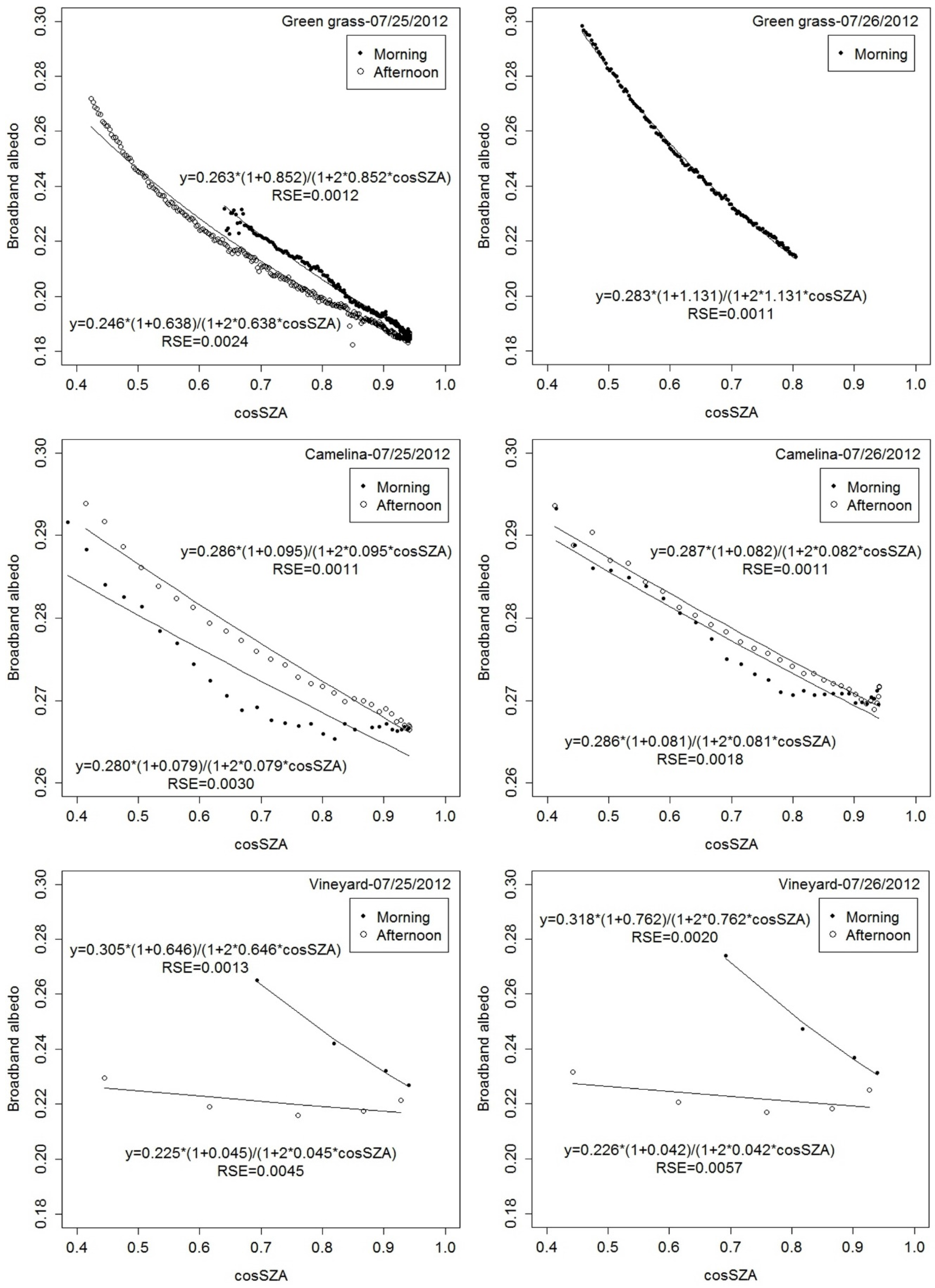
The broadband albedo was obtained as the ratio of the outgoing shortwave radiation to the incoming shortwave radiation measured at three sites: a green grass field, a camelina field, and a vineyard. The time interval between two consecutive measurements was different for each site: 1 min in the green grass, 10 min in the camelina field, and 1 h in the vineyard. It is well known that the surface albedo is dependent on the time of day because it depends strongly on the SZA. The dependence of broadband albedo on the SZA is shown in Figure 5 for the three sites. For each site and for each day, the results are grouped into morning (until 12 UTC) and afternoon (after 12 UTC) measurements. No measurements were taken in the afternoon on 26 July at the green grass site. At the three sites, the albedo decreases from dawn to noon, reaches a minimum value at noon, and then increases again until dusk. This behavior has been explained before by an increase in diffuse irradiance resulting from the increased scattering associated with longer path lengths at high solar zenith angles [20]. The obtained albedo dependence on SZA has also been observed in wheat fields using an albedometer [20] and in green crops and yellow grass using albedometers consisting of pyranometers [45]. The most exhaustive field data collection can be found in Yang et al. [37], which provides albedo data collected between 1997 and 2005 from a wide range of surface types (pastures, grasses, bare soil, prairie grasses with a few trees, rocky desert with scrub vegetation, pasture grasses with a few deciduous trees, grasses, crops, and prairie grasses). In all cases, the albedo shows a diurnal cycle similar to those depicted in Figure 5. Similar diurnal cycles have been observed in the spectral albedo measured using a multi-filter radiometer on short green grass at different times of the year [46] and for several wavelengths in the visible and NIR bands. The variation in the spectral albedo with SZA increased with increasing wavelength. The decrease in the broadband albedo with decreasing SZA from dawn to noon was obtained using a Bidirectional Reflectance Factor (BRF) library and some conversion formulas used in satellite broadband albedo calculations [47]. In this case, the same general trend was observed over a variety of surfaces, including grey gravel, dry sand, new snow, dry old snow, very wet melting snow, moss, lichen, lingonberry, and wet and dry peat.
Regarding the albedo parameterization as a function of the SZA, the field-measured albedo values were fitted to Equation (11). The results of the fits are given in Table 2. Briegleb [39] and Hou et al. [48] proposed d = 0.1 and 0.4 for surface types where the dependence of albedo on SZA is weak and strong, respectively. However, the d values found in the literature are significantly larger (0.5–1.1) [37]. The difference in the albedo-SZA relationship between morning and afternoon observations has been studied [37], and the research suggests that the albedos in the morning are not always larger than those in the afternoon. In any case, it is not our aim to gain insight into the physical basis of the parameterization of the broadband albedo as a function of the SZA. At this stage, we only wish to find the most suitable parameterization to interpolate the field data. However, we need to study the dependence of a and d on the surface type and compare their values with those obtained by other authors to confirm that our field data are dependable. When using Equation (11), field data with very high SZA and high albedo values were discarded [37,49,50], keeping only the field data with ρ < 0.3 and cos SZA > 0.385 (corresponding to SZA < 67°) for the camelina and cos SZA > 0.421 (corresponding to SZA < 65°) for the green grass site and the vineyard. The fitting results are given in Figure 5 for both the morning and afternoon data.
The statistical significance of a and d in Table 2 was tested (with a significance level of 5%) using the p-value test. Only afternoon d values for the vineyard failed the test. This means that Equation (11) explains the SZA dependence of the albedo for the three sites in the given range of SZA, except for the vineyard data in the afternoon. As shown in Table 2, a is similar in the three covers (0.2–0.3). In contrast, d is very different in the three cases, i.e., approximately 0.1 for the camelina field, between 0.6 and 1.1 for the green grass field, and between 0.6 and 0.8 for the vineyard morning data. A value of d = 0.1 is the lowest limit proposed by Briegleb [39] and Hou et al. [48], whereas the highest values are similar to those obtained by other authors [37]. Furthermore, there is no clear trend from morning to afternoon in the data [37]. The values of the field-measured albedos obtained using Equation (11) are shown in Table 3. The values are given for the time of the flights. The value of the SZA for each time was obtained using a solar position calculator [51]. The values of the albedo from 26 July are slightly larger than those from 25 July at the three sites. This small difference can be explained by some high clouds in the area on 25 July 2012.
Having proven the goodness of fit in the morning data in the three covers, the field data at the time of the flights were interpolated using Equation (11), with a and d corresponding to the morning fits.

3.2. Airborne Broadband Albedo

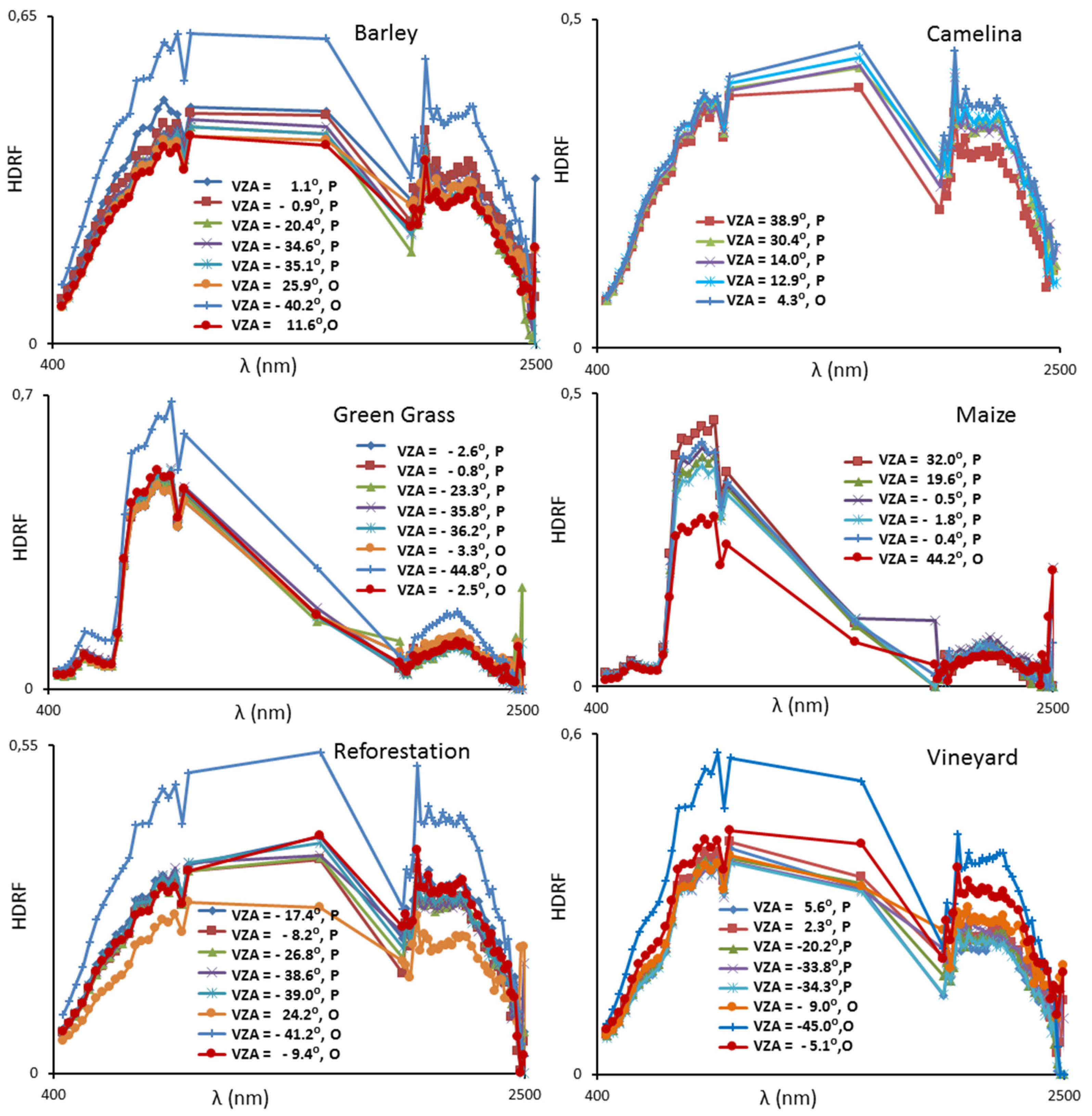
To estimate the broadband albedo from the airborne data, first we need to know the narrowband albedo. Because of the lack of angular measurements, the albedo cannot be calculated from the integration of the BRDF. In this work we use the HDRF as a proxy for the narrowband albedo. In Figure 6, we show the dependence of the HDRF on the VZA and flight direction, of pixels from sites with the following land covers: barley, camelina, green grass, maize, reforestation, and vineyard. Let us remember that −45° < VZA < 45°. The pixels on the camelina field, the green grass, and the vineyard were chosen at the exact location where the albedo field measurements were taken. The other sites were chosen to have a wider range of land covers to evaluate the HDRF dependence on the VZA. For the sake of clarity, we only show flights on 25 July 2012. Similar results were obtained for the flights on 26 July 2012. In the case of the barley field, all HDRF spectra are quite similar except the one at VZA = −40.2° for an orthogonal plane. HDRF seems to be VZA-independent for parallel flights as well as for orthogonal flights with positive VZA values up to 25.9°. The HDRF for the camelina site appears to be VZA-independent in the range of 400–1000 nm for the flights along the solar principal plane, even for VZA values as high as 38.9° and for flights perpendicular to the solar plane, as long as VZA is positive and small. However, the HDRF dependence on VZA becomes more apparent with increasing wavelength. The camelina site was out of the swath of the flights at 8:43, 8:51 and 9:46 UTC. In the case of the green grass, a very good match is observed over the spectral range of 400–2500 nm for all the parallel flights and for the orthogonal flights with small VZA. The flight at 9:38 UTC (orthogonal to the solar principal plane and with a VZA of −44.8°) exhibits HDRF values well above the others. We can conclude that the HDRF does not depend on the VZA for flights along the solar principal plane. For flights orthogonal to the solar principal plane, HDRF does not depend on the VZA as long as the VZA is small (−2.5°). The HDRF does show, however, a strong VZA dependence for flights orthogonal to the solar principal plane with high VZA values. The results for the vineyard are similar to those for the green grass. In the case of the maize, the HDRF appears to be VZA-independent for parallel flights and for orthogonal flights at low VZA. An important discrepancy is observed in the near-infrared band for a perpendicular flight with VZA = 44.2°. The HDRF spectra for the reforestation field do not show any VZA dependence for parallel flights; however, directional effects are observed with increasing VZA for orthogonal flights. In the case of flights orthogonal to the solar principal plane, for the barley we obtained HDRF (11.6°) < HDRF (25.9°) < HDRF (−40°), for the green grass HDRF (−2.5°) ≈ HDRF (−3.3°) < HDRF (−44.8°), for the reforestation HDRF (24.2°) < HDRF(−9.4°) < HDRF(−41.2°) and for the vineyard HDRF(−9°) < HDRF (−5°) < HDRF (−45°) over the whole spectral range. In all the cases we observe an increase of HDRF with an increase in the absolute value of VZA, especially for negative VZA (target observed in the backscattering direction). This trend can be explained by the combined action of the gap effect and the absence of shadows in the backscattering direction [21,22,24]. In the case of flights parallel to the solar principal plane, no clear trend is observed. It is well known that in this case the reflectance is symmetrical with respect to the nadir viewing direction and changes smoothly [21,22].
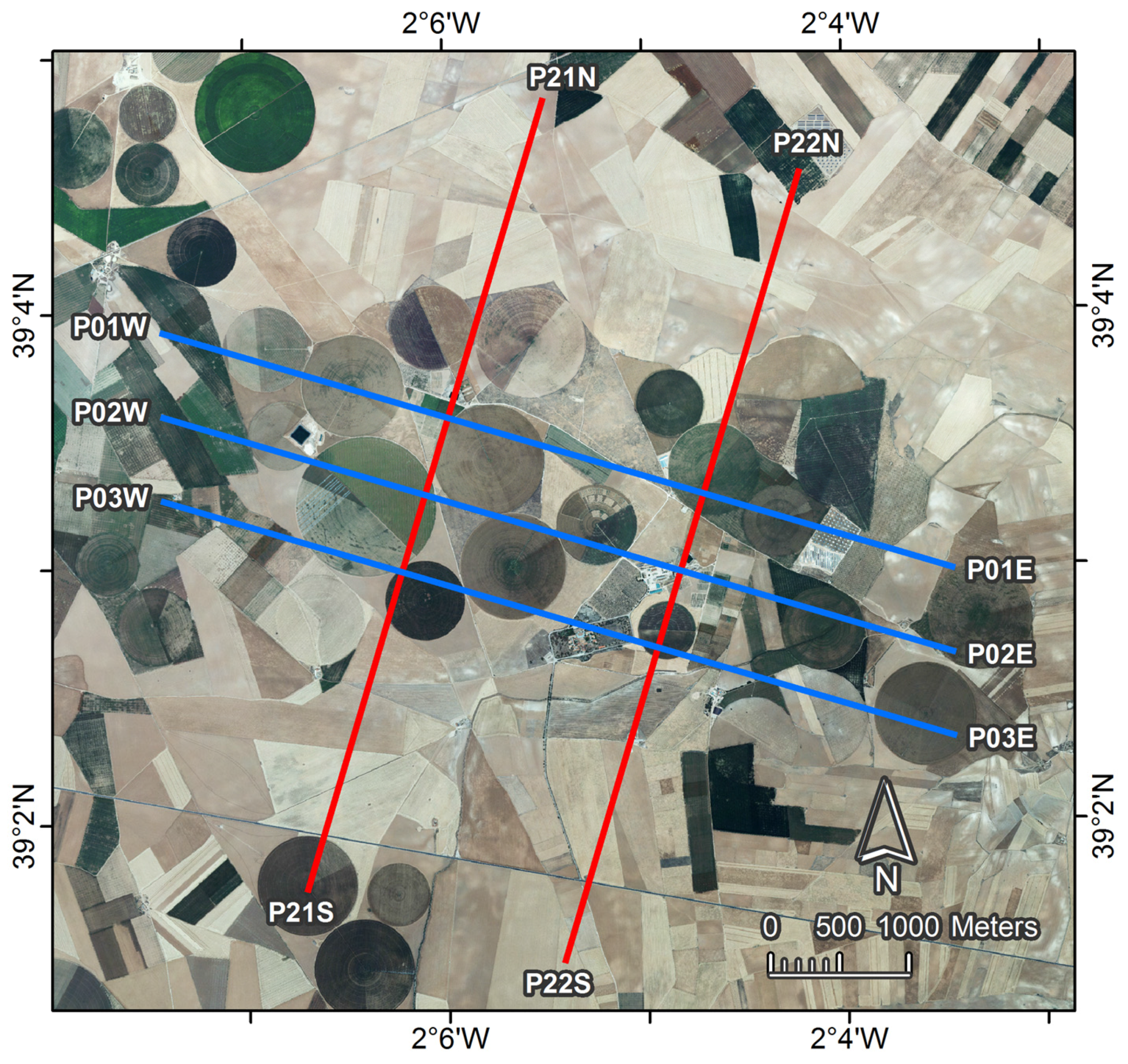
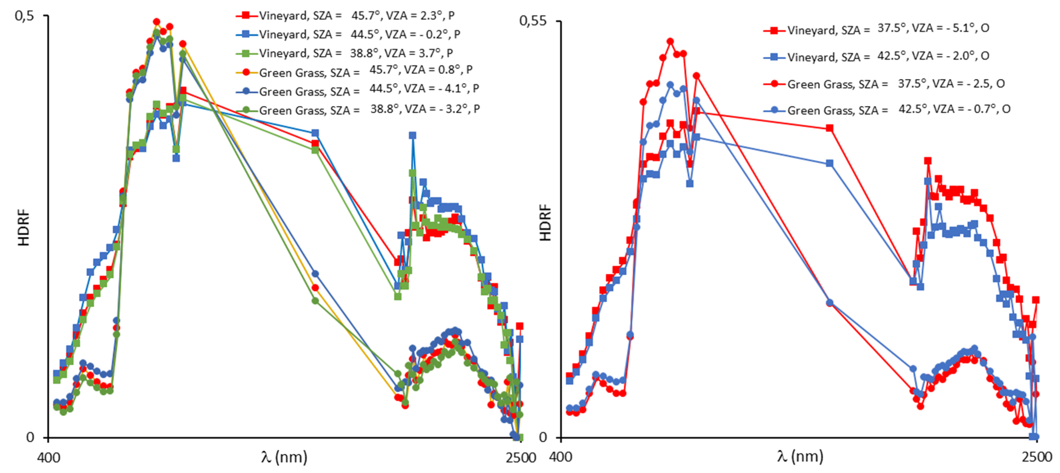
In order to study the airborne HDRF dependence on the SZA we take advantage of the fact that some flight lines of 25 July are nearly superimposed to flight lines of 26 July taken at different UTC, which allows the observation of a given area with very close values of VZA and different SZA. The results for the green grass and the vineyard and for VZA close to nadir are shown in Figure 7. These two sites were chosen because of their different canopy architecture (the vineyard is a field with a high 3D structured canopy, while the green grass is a cover with continuous and dense canopy) and because the VZA is very close to 0°, and HDRF changes very smoothly around nadir [21]. The results show that the HDRF depends on the SZA very slightly for flights parallel to the solar principal plane. On the other hand, HDRF dependence on the SZA is more important for flights perpendicular to the solar principal, especially for the green grass in the NIR and for the vineyard in the SWIR. On the other hand, it is worth noting that the HDRF for flights parallel to the solar principal plane attains virtually the same values on 25–26 July. Thus, the possible changes of the atmospheric conditions between both dates might have a negligible influence on the HDRF.
These results show that the narrowband albedo can be approximated by the HDRF for flights along the solar principal plane for any VZA. In the case of flights orthogonal to the solar principal plane, the approximation is not valid for high VZA values, especially if the VZA is negative. It is worth noting that a negative VZA value for orthogonal planes means that the sensor detects backscattered radiation from the target. Directional effects become more important in the backscattering direction. We will take into account this fact in the validation. We have tested the dependence of HDRF on VZA at only six sites. Still, we assume that the results obtained from these sites can be extrapolated to the entire study area. Authors interested in a particular area should first check the HDRF dependence on the VZA and on the SZA.
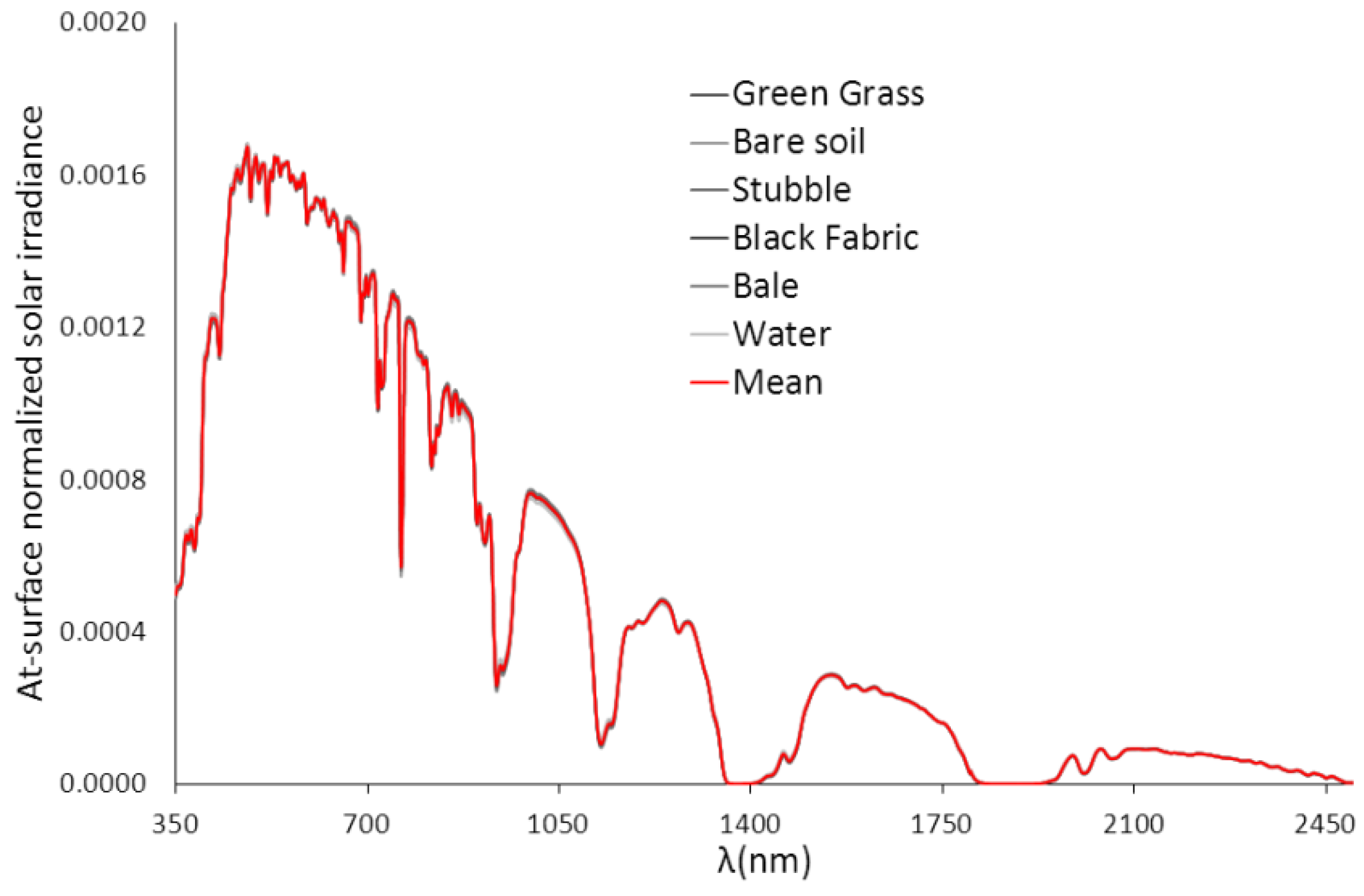
To calculate the Integrated Albedo, the reflected downwelling irradiance from the white panel was used. We calculated the mean value of the ASD measurement on the white reference panel on the sites where ASD measurements were taken. The results are shown in Figure 8. It is worth noting that the normalized spectrum varies very little from site to site. The mean value was used to calculate the weighting factors.
Some authors have used the calculated top of atmosphere solar irradiance [15] or a calculated at-surface solar irradiance [13,20] in their broadband albedo calculations. Using the at-surface downwelling reflected irradiance from the white panel means that we are measuring the apparent albedo, which is the albedo that can be compared with the field measurements [13,18], as opposed to inherent albedo [18]. The weighting coefficients for each channel in Equation (10) are given in Table 4, along with the central wavelength and the bandwidth of each channel. Channels 22 and 23 are at the edge of the atmospheric windows, and they have a low SNR and are seldom useful. Channels 44 and 46 had a very low SNR due to sensor malfunction [34]. We calculated the weighting coefficients disregarding channels 22, 23, 44, and 46 following the procedure described in the previous section, to cover the resulting gaps equally between the neighboring channels. The Integrated Albedo presented in this paper was calculated without taking into account channels 22, 23, 44, and 46.
The narrow-to-broadband albedo conversion can also be performed using other approaches. Many authors have used Equation (1) by taking ρi to be the bidirectional reflectance [52,53,54]. Broadband albedo for AHS has been normally calculated from the MODIS equation for apparent broadband albedo [7] (Equation (2)) or even in a simpler way from AHS channels 9 and 12 as ρ = 0.45ρ9 + 0.55ρ12 [55].
The Integrated Albedo and the MODIS Albedo are compared in five selected areas (Figure 9): the camelina field, the green grass field, the vineyard, a reforestation field, and a barley field. The first three were chosen because they are the validation sites. The reforestation and barley fields were chosen to include a wider range of albedo values. Although the albedometer in the camelina field was out of the swath of the flight at 9:46 UTC, the pixels in Figure 9 correspond to an area of the camelina field in the swath of the flight. To see the effect of the VZA and the flight direction on the albedo, we show the results for one flight parallel to the solar principal plane (flight at 9:02 UTC, Figure 9a) and another orthogonal to the solar principal plane (flight at 9:46 UTC, Figure 9b). The values provided by the two methods are very close to each other. When we compare the results for both flights, we observe that both methods exhibit similar behavior with respect to the VZA and the flight direction. In the case of the vineyard, values are larger for the flight at 9:46 UTC than at 9:02 UTC, whereas for the camelina field, the values are larger for the 9:02 UTC flight. In the case of the green grass, an increase in the values range is obtained for the flight at 9:46 UTC. Notably, the MODIS Albedo is slightly higher than the Integrated Albedo in the vineyard for both flights, while the opposite is true for the other sites. Similar results were obtained for the rest of the flights. It has also been reported [27] that MODIS albedo products overestimate the surface albedos of low-albedo sites and underestimates the albedos of high-albedo sites. The same trend is observed in Figure 9, which compares the Integrated and MODIS albedos. Let us remember that both the Integrated and the MODIS albedos use HDRF as a proxy for the albedo; the only difference between them lies in the narrow to broadband conversion. This bias could then be attributed to the narrow to broadband conversion procedure. Future albedo products should perhaps improve the narrow to broadband conversion algorithms. We conclude that a slight bias between the two methods exists. This bias may be responsible for the better albedo estimation of the Integrated Albedo, as we will see when estimating the uncertainty statistics of the two methods.
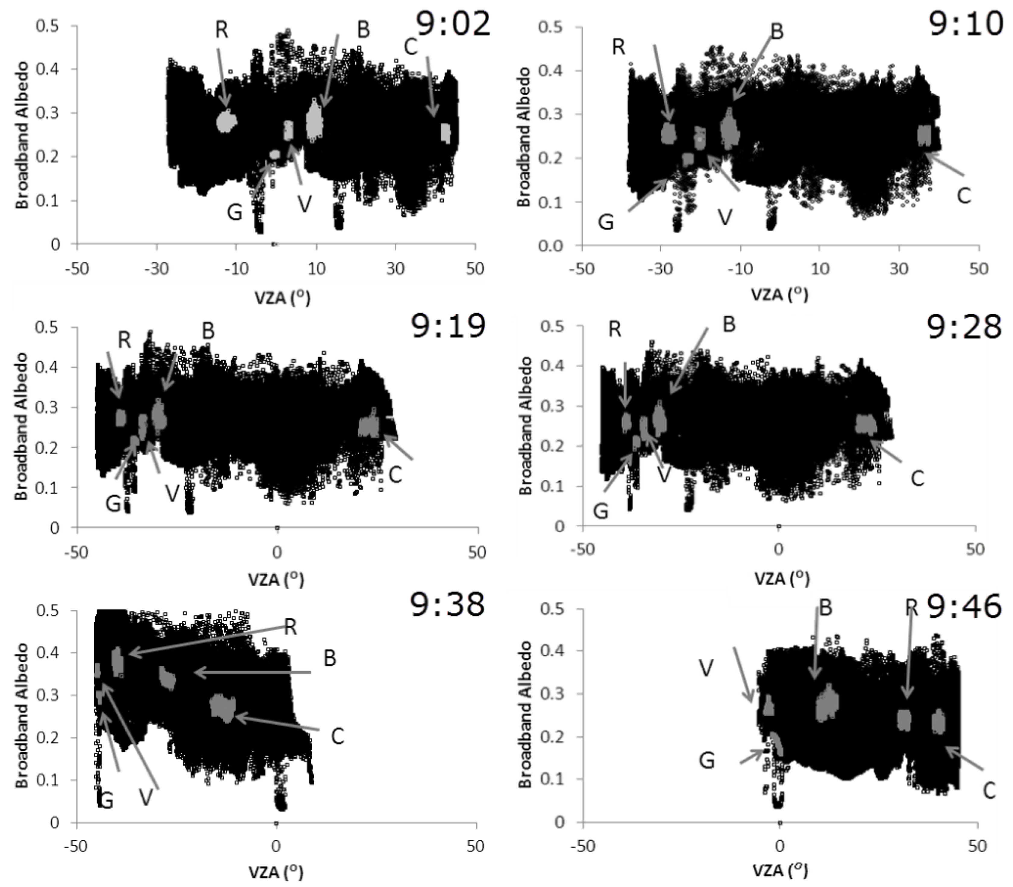
The angular dependence of the Integrated Albedo, calculated with the weighting coefficients of Table 4, is shown in Figure 10 for the overlapping area for the flights on 25 July 2012 at an altitude of 2000 m above ground level and with a spatial resolution of 5 m. Flights at 9:02, 9:10, 9:19, and 9:28 UTC are parallel to the solar principal plane, while flights at 9:38 and 9:46 UTC are orthogonal to the solar principal plane. Pixels corresponding to the five selected areas (vineyard, green grass, camelina field, reforestation field, and barley field) are displayed in different colors. In the case of the camelina, green grass, and vineyard, the areas marked in Figure 10 correspond to an area around the pixel that corresponds to the location of the field measurements. Because the broadband albedo does not depend on the viewing direction, the albedo of a certain location should be the same for all the flights (we expect small changes due to the change in the SZA). Therefore, a certain location should exhibit the same albedo regardless of the VZA under which it is observed, and regardless of the direction of the flight with respect to the solar principal plane. In this work, the Integrated Albedo is calculated assuming that HDRF varies very slightly with the viewing direction, and therefore, the narrowband albedo can be approximated by the HDRF. Figure 10 is intended to show the limits of validation of that approximation. For the flights at 9:02, 9:10, 9:19, 9:28, and 9:46 UTC, we can see that the Integrated Albedo of a certain location does not change much from one flight to another. It is obvious that the angular dependence becomes important for flights orthogonal to the solar principal plane and for backscattered radiation (i.e., the flight at 9:38 UTC). There is a very strong increase in the albedo of targets observed in the backscattering direction when the scanning takes place along the solar principal plane.

3.3. Validation

We now focus on the validation of the results. The Integrated Albedo and the MODIS Albedo will be compared to field data and to each other. The results of other authors are also discussed.
Regarding field measurements, we considered that 99% of the observed net radiation originated from a circle with a diameter of 10 times the sensor height [35,36]. This means that in the case of the camelina field, albedo measurements originate from a circle with a diameter of 10 m around the sensor; in the case of the green grass, from a circle with a diameter of 20 m; and in the case of the vineyard, from a circle with a diameter of 40 m. For validation, a window was selected around the pixel where the sensor was located with a size such that it contained the circle mentioned above. For the camelina field, for flights with a pixel of 5 m, we took the value of the albedo measured at the pixel where the sensor was located, while for flights with a pixel of 3 m, we selected a 3 × 3 pixel window around the pixel where the sensor was placed. For the green grass, a 5 × 5 pixel window around the location of the sensor was selected for the flights with 3-m pixels, and a 3 × 3 pixel window was selected for the flights with 5-m pixels. For the vineyard site, a 7 × 7 window was taken for the 5-m-pixel images and an 11 × 11 window was taken for the 3-m-pixel images. When comparing airborne with field data we must take into account that the spectral response of the field radiometers used in this work is from 305 to 2800 nm [36]. The airborne albedo has been calculated from 350 nm to 2500 nm. The at-surface solar irradiance is highly attenuated below 350 nm (close to the ozone absorption band centered at 260 nm) [56] (p. 97). In the range 2500–2800 nm the at-surface solar irradiance is negligible due to the strong absorption band of water centered at 2600 nm and that of CO2 centered at 2700 nm [56] (p. 95). Thus we assume that the field-measured albedo and the airborne albedo values can be compared. Field albedo values obtained with the same equipment have previously been compared to AHS albedo data over the same area [7].
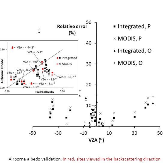
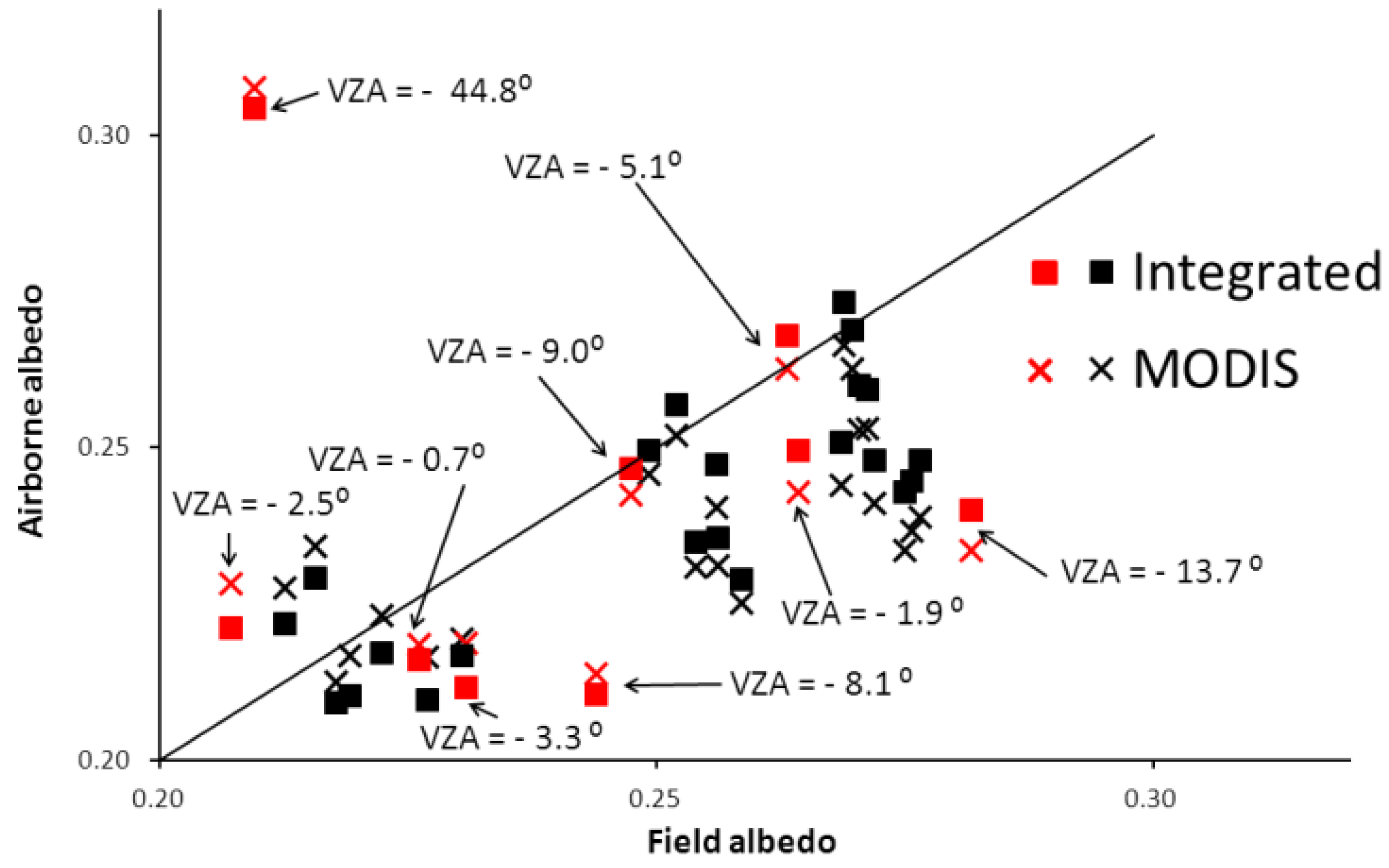
The validation results are shown in Figure 11 and Table 5. In Figure 11, the albedos corresponding to sites with negative VZA values and for flights orthogonal to the solar principal plane are marked in red and the corresponding VZA values are given. The highest estimated albedo was for the green grass and the flight at 9:38 UTC on 25 July 2012 (Integrated Albedo = 0.304, MODIS Albedo = 0.308). The green grass site was observed with a high VZA in the backscattering direction (VZA = −44.8°). In this case, the HDRF cannot be used as a proxy for the narrowband albedo, and the predicted values are clearly wrong. These results are consistent with Figure 10, in which we noticed an increase in albedo values for sites observed with high VZA in the backscattering direction. As for the rest of the airborne albedos, it is clear from Figure 11 that both the Integrated Albedo and the MODIS Albedo tend to underestimate the albedo value. This behavior has also been obtained in the validation of broadband albedo calculated from BRDF integration using AHS data on corn, wheat, and barley at the Barrax site [16], and it has also been reported in other works using the MODIS BRDF/albedo products [57,58]. The widespread obtained can be caused by the procedure used to obtain the field albedos at the time of the flights and the weather conditions. The scatter observed in Figure 5, especially in the camelina field, along with the differences observed between morning and afternoon field-measured albedo can be caused by atmospheric conditions, especially on 25 July, when high clouds were observed during the acquisition of the field data.
According to the Root Mean Square Error (RMSE) values (Table 5), the Integrated Albedo, relative to the MODIS albedo, provides better estimates in the case of the camelina and the vineyard sites and similar estimates in the case of the green grass. Previous validation results over wheat and barley fields [7] produced an RMSE of 0.01 for airborne albedo calculated using the MODIS formula with narrowband albedos calculated via BRDF integration. An RMSE of 0.03 was obtained for airborne albedo estimated using the MODIS formula with narrowband albedos approximated by HDRF. In the latter case, the larger discrepancies between airborne and field measurements were observed for values of VZA < 0 in the backscattering direction. No major distinction was found between the two procedures for other VZA values.
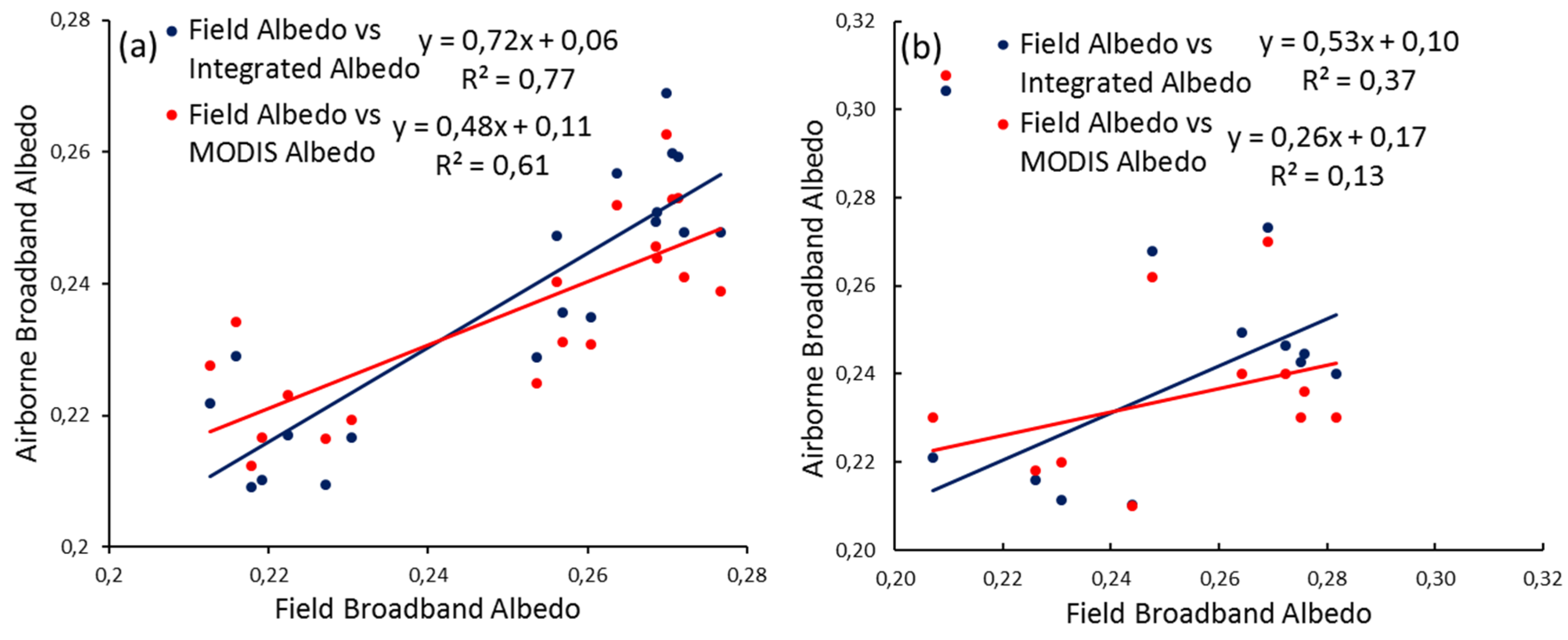
A careful distinction must be made between the flights parallel to the solar principal plane and those orthogonal to the solar principal plane. We have compared field-measured albedo with airborne albedo from parallel and orthogonal flights separately. The correlation between field and airborne albedo is much better for flights parallel to the solar principal plane than for the orthogonal ones (Figure 12) both for the Integrated Albedo and the MODIS Albedo. The coefficient of determination is greater for the parallel flights than for the orthogonal ones. Moreover, the slope of the fit line is closer to one and the intercept is smaller for the parallel flights. The RMSE values of the validation in separate sets are given in Table 6. The approximation of using the HDRF as a proxy for the narrowband albedo yields better results for the flights parallel to the solar principal plane, because the HDRF depends slightly on the VZA and the SZA for these flights as previously shown. The HDRF is highly anisotropic for flights orthogonal to the solar principal plane, particularly for high VZA values, what explains the large scatter in the data of Figure 12b and the worse results of the fit.
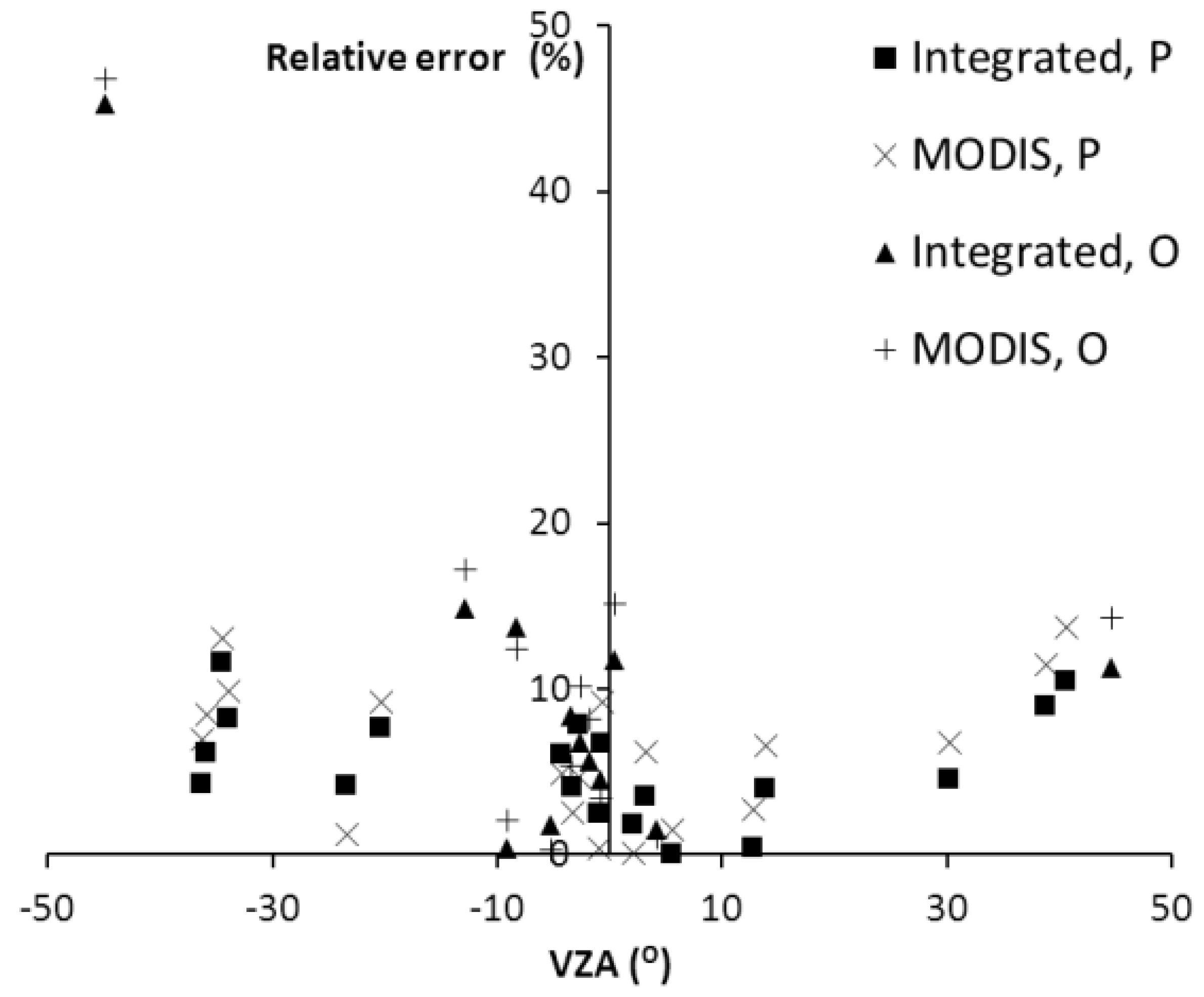
We estimated the discrepancy between airborne and field data by computing the relative error (taking the field value as the true value) for each validation datum using the following equation:
R e l a t i v e   e r r o r   ( % ) = | ρ a ρ f | ρ f   × 100
where ρa is the airborne albedo and ρf is the field albedo. The relative error as a function of VZA is shown in Figure 13, with data classified according to the procedure used for albedo estimation (Integrated or MODIS) and the flight direction (either parallel or orthogonal to the solar principal plane). The values for the three sites are plotted in the same figure. It is worthwhile noting that the relative error using the integration method is smaller than that using the MODIS formula in most of the cases. The relative error for flights parallel to the solar principal plane shows a slight increase with increasing VZA. For positive VZA values, the relative error of the Integrated Albedo remains below 11%, even for the VZA values as high as 40.8°, while for negative VZA values, the relative error remains below 12% for VZA values as high as −36.2°. For flights orthogonal to the solar principal plane, a relative error of 45% is obtained for VZA = −45° (corresponding to the green grass), while for the rest of the VZA values (between −13° and 45°), the relative errors remain below 15%. Backscattered light becomes the main source of error in albedo calculations, as previously noted [7]. It is worth noting that the propagation of the error in the albedo to other physical quantities in the surface energy budget has been studied [7], and three scenarios were considered according to the albedo relative error: low (21%), medium (43%), and high (65%). Our results would be classified in the low error scenario. The fact that we use the at-surface solar irradiance to calculate the contribution of each AHS channel in the integration method is an advantage that may explain the good results.
Now we proceed to compare our results with previous results. As for the validation of remote sensing albedo data, numerous results for sensors on satellite platforms have been published. However, very few results can be found concerning airborne sensors. Most of the MODIS albedo product validation results attribute the discrepancy between satellite and field data to the heterogeneity of MODIS pixels, and some authors noted the need for high spatial resolution albedo estimates to improve the validation procedure. Authors using airborne data carry out the narrow to broadband conversion using linear combinations that were devised for satellite sensors, despite the spectral mismatch between the sensors. Additionally, for the narrow to broadband conversion, some authors use the equation proposed in Liang et al. [18], while others use Equation (2) in this paper. Liang et al. [59] use the Narrow-to-Broadband algorithm to MODIS and apply Equation (1) to estimate the apparent broadband albedo. The validation is carried out over a diverse set of surfaces, including soils, crops, and natural vegetation, throughout the year, and an RMSE of 0.018 is obtained, a value higher than the one obtained in this work. Jacob et al. [60] calculated the albedo from the airborne sensor POLDER with a spatial resolution of 20 m using three BRDF models. They perform the narrow to broadband albedo conversion using a linear combination of spectral hemispherical reflectance. They use several sets of coefficients that were proposed in the literature for different sensors with spectral response functions different from those of POLDER. The validation was performed over several sites with three covers: alfalfa, sunflower, and wheat. A relative accuracy of 9% is obtained when using the appropriate set of coefficients. They obtain an RMSE in the range of 0.02–0.05, depending on the BRDF model and the combination of coefficients used in the computation of the broadband albedo. Moreover, they study the RMSE for a given BRDF model and for different sets of coefficients in the narrow to broadband conversion and obtain the same range of variation in the RMSE (0.02–0.05) depending on the set of coefficients used. Thus, it seems that the narrow to broadband albedo conversion is a very important source of errors. This emphasizes the need to develop a specific algorithm to convert narrow albedo to broadband albedo for each sensor, as we propose in our work.
Jin et al. [61] evaluated the accuracy of MODIS surface albedo using BRDF modeling and field measurements over the SUFRAD [62] and CART/SGP [63] sites. They obtain an RMSE = 0.018 over the SUFRAD stations and an RMSE = 0.015 for the CART/SGP sites. In this case, they obtain the inherent albedo, because the narrow to broadband albedo conversion is carried out using the linear combination in Liang [15]. A larger difference between MODIS and field values is observed in winter, late fall, and early spring than in the growing seasons, suggesting the possible effect of heterogeneity within the MODIS pixels. This justifies the need for albedo estimations using data with higher spatial resolution, as in this work.
Liu et al. [58] carry out a comparison of MODIS albedo with field albedo for three SZA ranges (local noon, 55° < SZA < 65°, and 75° < SZA < 85°) on snow-free surfaces at six sites over a three-year period. Several land cover types were tested, including agriculture, grassland, pasture, and a mixture of grassland and shrubland. They obtain an RMSE = 0.012–0.1, depending on the homogeneity of the area. The agreement between the remote sensing albedo and field albedo is best when the SZA is small (<30°). In the present study, we work with 37.5° < SZA < 49.3° and we obtain lower RMSE values. They observed that MODIS underestimates the surface albedo. Wang et al. [64] evaluate the accuracy of MODIS V004 and V005 shortwave and visible albedo products for 18 FLUXNET [65] sites between 2000 and 2007. They calculate the inherent broadband albedo as a linear combination of narrowband albedos using the coefficients in Liang et al. [18]. In the case of the shortwave albedo (400 to 3000 nm), i.e., the albedo that can be compared to our results, they obtained a bias of −0.009 and a standard deviation of 0.02 for the V004 product and a bias of −0.008 and a standard deviation of 0.02 for the V005 product. They find that the difference between the ground and MODIS albedos is larger at heterogeneous sites. The differences between satellite- and ground-measured albedos have been analyzed as a function of surface heterogeneity, plant functional type and seasonality at the FLUXNET sites by Cescatti et al. [27]. Only sites with the highest degree of homogeneity in the area surrounding the measurement tower were chosen, and only sites with a single plant functional type were included in the analysis. They observe that MODIS overestimates the surface albedo of low-albedo sites and underestimates the albedo of high-albedo sites. We obtained the same result when comparing the MODIS Albedo and the Integrated Albedo data (Figure 8). Therefore, according to our results, this behavior can be partly attributed to the narrow to broadband conversion algorithm. Cescatti et al. [27] obtain a mean absolute percentage error between 5% and 40%, with the lowest values at the most spatially homogeneous sites. Their results demonstrate the need to characterize the spatial heterogeneity of ground sites using airborne and finer-scale satellite imagery. Some authors have evaluated the MODIS/Albedo MCD43 product and the AHS albedo over the same area used in our study [16]. Two BRDF models have been applied to the AHS data to obtain the narrowband albedo: the RossThick-LiSparse-Reciprocal model (the one used in the MODIS/Albedo MCD43 product) and the RossThick-Maignan-LiSparse-Reciprocal model, which corrects for the hot spot effect. The broadband albedo was then calculated using Equation (1). To compare the AHS and MODIS albedo values, the AHS images are aggregated to simulate the MODIS pixel size. When compared to field data, the non-aggregated AHS data produce an RMSE = 0.018 for both BRDF models. In addition to this, both models underestimate the albedo. The aggregated AHS albedo versus MODIS albedo yields an RMSE = 0.04 for both models. The discrepancy between the aggregated and MODIS albedo is attributed not only to the aggregation procedure but also to the fact that MODIS combines data from different dates, while AHS uses data from a single date. Airborne sensors have been used in the validation of satellite albedo data. For instance, MODIS and Landsat albedo retrievals were validated based on comparisons with field and airborne albedos, using the Cloud Absorption Radiometer (CAR) airborne sensor [28]. Satellite and airborne albedos were estimated using the BRDF modeling, and ground measurements were taken over the ARM/CART site [66]. When compared with field measurements, they obtain an RMSE of 0.009 for MODIS when SZA < 45° and 0.03 when SZA > 45°. In the case of the CAR sensor, which has a spatial resolution of 30 m, the RMSE = 0.01 for SZA < 45° and 0.03 for SZA > 45°. The results for Landsat yield an RMSE = 0.03 for SZA < 45° and 0.04 for SZA > 45°. In their work, they propose the use of the airborne albedos as ground-truth data for satellite albedo validation. This point explains the need for an algorithm to estimate the broadband albedo using airborne hyperspectral data with high spatial resolution. The Direct-Estimation algorithm has been applied to Airborne Visible Infrared Imaging Spectrometer (AVIRIS) data [19], yielding an RMSE = 0.03 when their data are compared to ground data. They study the effect of surface anisotropy on the broadband albedo estimation and conclude that Lambertian approximation does not lead to significant errors over snow-free surfaces.

4. Conclusions

The broadband albedo of the AHS data over the Barrax site (Spain) has been calculated using a new operational method and then validated using field measurements from three sites: a camelina field, a green grass field, and a vineyard. The method is based on the integration of the HDRF over the spectral range of 350–2500 nm. The spectral response functions of the AHS channels and the at-surface downwelling irradiance measured on a white reference panel were used in the integration. The method does not need any BRDF modeling, does not require multiangular measurements, and it is based on the assumption that the narrowband albedo can be approximated by the HDRF. To assess this approximation, the dependence of the airborne HDRF on the VZA and on the SZA was evaluated at the validation sites for VZA values between −45° and 45°. The results show that the narrowband albedo can be approximated by the HDRF for flights parallel to the solar principal plane for all VZA values. For flights orthogonal to the solar principal plane, the approximation is valid for all positive VZA values (forward scattering direction). However, the data from flights orthogonal to the solar principal plane with negative VZA values in the green grass and vineyard demonstrate that the HDRF does not depend on the viewing direction for VZA values up to −9.0°, while a significant VZA dependence is observed for VZA = −45°.
For validation purposes, albedo field measurements were obtained at the same time as the flights. Measurements were taken every 10 min at the camelina site, every minute at the green grass site, and every hour at the vineyard site. A parameterization of the field albedo as a function of the SZA was used to calculate the field albedo at the time of the flights. The albedo obtained via the integration of the HDRF (Integrated Albedo) was compared to that obtained using the equation for the broadband apparent albedo proposed for MODIS after adaptation to the AHS data (MODIS Albedo). Although the values obtained by both methods are very similar, a slight bias exists, the sign of which depends on the land cover. For validation, the RMSE and the relative errors were calculated. A lower RMSE was obtained using the Integrated Albedo than using the MODIS Albedo for the camelina (0.013–0.018 vs. 0.018–0.02) and the vineyard (0.012–0.016 vs. 0.015–0.018), while similar RMSE values were obtained for the green grass (0.009–0.013). The relative error of the Integrated Albedo is lower than that of the MODIS Albedo for the majority of the validation data, especially for those at high VZA values. These results improve upon previous results using the AHS sensor over the same area (RMSE = 0.01–0.03). When the validation is carried out for parallel and perpendicular flights separately, we obtain lower RMSE values and a higher coefficient of determination for the flights parallel to the principal plane. Moreover, the relative error in the Integrated Albedo is less than 12% for −36.2° < VZA < 40.8° in the case of flights parallel to the solar principal plane and less than 15% for −13° < VZA < 45° and 45% for VZA = −45° for flights orthogonal to the solar principal plane. We conclude that the method can be used for −45° < VZA < 45° in the case of flights parallel to the solar principal plane. In the case of flights orthogonal to the solar principal plane, it can be used for −13° < VZA < 45°; however, it should be used with caution for VZA values close to −45°.
Previous broadband albedo calculations using the AHS sensor relied on the MODIS apparent broadband albedo equation without considering the spectral mismatch between MODIS bands and AHS channels. Although the use of this equation produces good albedo estimates, its use with the AHS sensor has never been justified. In this work, we have carried out a unique comparison of the Integrated Albedo to the MODIS Albedo, proving that the Integrated Albedo provides better albedo estimates (lower RMSEs and lower relative errors). At the same time, this study can be considered to be a justification for using the MODIS equation with the AHS sensor.
The authors propose the use of the weighting coefficients calculated for each AHS channel over the at-surface solar spectrum for the calculation of the broadband albedo when using data from the REFLEX campaign. Future investigations should be conducted to extend the application of the method to other sensors and to a wider range of VZA values.

Acknowledgments

The research leading to these results has received funding from the European Community’s 7th Framework Program (FP7/2008-2013) under EUFAR contract No. 27159, Cost Action ES0903-EUROSPEC and ESA Grant D/EOP/rp/2012/48.

Author Contributions

J.F.C. conceived the idea of the work, calculated the albedo images using the two procedures described in the paper, processed the field data to obtain the field albedos, and calculated the parameterization as a function of the VZA. He carried out the validation and the statistical analysis and wrote and edited the paper. C.R. performed the fits of the albedo field values to the parameterization function and discussed the values of the parameters. J.P. calculated the VZA of each pixel in each image and contributed to the editing of the figures and the references. F. de la Cruz provided details on the field experimental devices, and J.R.-P. provided information on the operation of the radiation meters. S.F. contributed to the critical analysis of the paper. All authors contributed to the manuscript by writing, editing, and proofreading.

Conflicts of Interest

The authors declare no conflict of interest.

References

  1. Norman, J.M.; Kustas, W.P.; Humes, K.S. Source approach for estimating soil and vegetation energy fluxes in observations of directional radiometric surface temperature. Agric. For. Meteorol. 1995, 77, 263–293. [Google Scholar] [CrossRef]
  2. Allen, R.G.; Tasumi, M.; Trezza, R. Satellite-based energy balance for mapping evapotranspiration with internalized calibration (metric)—Model. J. Irrig. Drain. Eng. 2007, 133, 380–394. [Google Scholar] [CrossRef]
  3. Zhang, X.; Liang, S.; Wang, K.; Li, L.; Gui, S. Analysis of global land surface shortwave broadband albedo from multiple data sources. IEEE J. Sel. Top. Appl. Earth Observ. Remote Sens. 2010, 3, 296–305. [Google Scholar] [CrossRef]
  4. Zhang, Y.C.; Rossow, W.B.; Lacis, A.A. Calculation of surface and top of atmosphere radiative fluxes from physical quantities based on ISCCP data sets 1. Method and sensitivity to input data uncertainties. J. Geophys. Res. 1995, 100, 1149–1165. [Google Scholar] [CrossRef]
  5. Myhre, G.; Myhre, A. Uncertainties in radiative forcing due to surface albedo changes caused by land-use changes. J. Clim. 2003, 16, 1511–1524. [Google Scholar] [CrossRef]
  6. Sellers, P.J.; Meeson, B.W.; Hall, F.G.; Asrar, G.; Murphy, R.E.; Schiffer, R.A.; Bretherton, F.P.; Dickinson, R.E.; Ellingson, R.G.; Field, C.B.; et al. Remote sensing of the land surface for studies of global change: Models—Algorithms—Experiments. Remote Sens. Environ. 1995, 51, 3–26. [Google Scholar] [CrossRef]
  7. Mattar, C.; Franch, B.; Sobrino, J.A.; Corbari, C.; Jimenez-Munoz, J.C.; Olivera-Guerra, L.; Skokovic, D.; Soria, G.; Oltra-Carrio, R.; Julien, Y.; et al. Impacts of the broadband albedo on actual evapotranspiration estimated by S-SEBI model over an agricultural area. Remote Sens. Environ. 2014, 147, 23–42. [Google Scholar] [CrossRef]
  8. Timmermans, W.J.; Kustas, W.P.; Anderson, M.C.; French, A.N. An intercomparison of the surface energy balance algorithm for land (SEBAL) and the two-source energy balance (TSEB) modeling schemes. Remote Sens. Environ. 2007, 108, 369–384. [Google Scholar] [CrossRef]
  9. Gonzalez-Dugo, M.P.; Neale, C.M.U.; Mateos, L.; Kustas, W.P.; Prueger, J.H.; Anderson, M.C.; Li, F. A comparison of operational remote sensing-based models for estimating crop evapotranspiration. Agric. For. Meteorol. 2009, 149, 1843–1853. [Google Scholar] [CrossRef]
  10. Bastiaanssen, W.G.M.; Menenti, M.; Feddes, R.A.; Holtslag, A.A.M. A remote sensing surface energy balance algorithm for land (SEBAL)-1. Formulation. J. Hydrol. 1998, 212, 198–212. [Google Scholar] [CrossRef]
  11. Roerink, G.J.; Su, Z.; Menenti, M. S-sebi: A simple remote sensing algorithm to estimate the surface energy balance. Phys. Chem. Earth Part B Hydrol. Oceans Atmos. 2000, 25, 147–157. [Google Scholar] [CrossRef]
  12. Colaizzi, P.D.; Kustas, W.P.; Anderson, M.C.; Agam, N.; Tolk, J.A.; Evett, S.R.; Howell, T.A.; Gowda, P.H.; O’Shaughnessy, S.A. Two-source energy balance model estimates of evapotranspiration using component and composite surface temperatures. Adv. Water Resour. 2012, 50, 134–151. [Google Scholar] [CrossRef]
  13. Tasumi, M.; Allen, R.G.; Trezza, R. At-surface reflectance and albedo from satellite for operational calculation of land surface energy balance. J. Hydrol. Eng. 2008, 13, 51–63. [Google Scholar] [CrossRef]
  14. Qu, Y.; Liang, S.; Liu, Q.; He, T.; Liu, S.; Li, X. Mapping surface broadband albedo from satellite observations: A review of literatures on algorithms and products. Remote Sens. 2015, 7, 990–1020. [Google Scholar] [CrossRef]
  15. Liang, S. Narrowband to broadband conversions of land surface albedo I algorithms. Remote Sens. Environ. 2000, 76, 213–238. [Google Scholar] [CrossRef]
  16. Sobrino, J.A.; Franch, B.; Oltra-Carrió, R.; Vermote, E.F.; Fedele, E. Evaluation of the MODIS albedo product over a heterogeneous agricultural area. Int. J. Remote Sens. 2013, 34, 5530–5540. [Google Scholar] [CrossRef]
  17. Schaaf, C.B.; Gao, F.; Strahler, A.H.; Lucht, W.; Li, X.; Tsang, T.; Strugnell, N.C.; Zhang, X.; Jin, Y.; Muller, J.P.; et al. First operational BRDF, albedo nadir reflectance products from MODIS. Remote Sens. Environ. 2002, 83, 135–148. [Google Scholar] [CrossRef]
  18. Liang, S.; Strahler, A.H.; Walthall, C. Retrieval of land surface albedo from satellite observations: A simulation study. J. Appl. Meteorol. 1999, 38, 712–725. [Google Scholar] [CrossRef]
  19. He, T.; Liang, S.; Wang, D.; Shi, Q.; Tao, X. Estimation of high-resolution land surface shortwave albedo from AVIRIS data. IEEE J. Sel. Top. Appl. Earth Observ. Remote Sens. 2014, 7, 4919–4928. [Google Scholar] [CrossRef]
  20. Disney, M.; Lewis, P.; Thackrah, G.; Quaife, T.; Barnsley, M. Comparison of MODIS broadband albedo over an agricultural site with ground measurements and values derived from earth observation data at a range of spatial scales. Int. J. Remote Sens. 2004, 25, 5297–5317. [Google Scholar] [CrossRef]
  21. Kuusk, A. The angular distribution of reflectance and vegetation indices in barley and clover canopies. Remote Sens. Environ. 1991, 37, 143–151. [Google Scholar] [CrossRef]
  22. Camacho de Coca, F.; Gilabert, M.A.; Meliá, J. Bidirectional reflectance Factor Analysis from Field Radiometry and Hymap Data; European Space Agency: Paris, France, 2001; p. 163. [Google Scholar]
  23. Gao, F.; Schaaf, C.B.; Strahler, A.H.; Jin, Y.; Li, X. Detecting vegetation structure using a kernel-based BRDF model. Remote Sens. Environ. 2003, 86, 198–205. [Google Scholar] [CrossRef]
  24. Weyermann, J.; Damm, A.; Kneubuhler, M.; Schaepman, M.E. Correction of reflectance anisotropy effects of vegetation on airborne spectroscopy data and derived products. IEEE Trans. Geosci. Remote Sens. 2014, 52, 616–627. [Google Scholar] [CrossRef]
  25. Román, M.O.; Gatebe, C.K.; Schaaf, C.B.; Poudyal, R.; Wang, Z.; King, M.D. Variability in surface BRDF at different spatial scales (30 m–500 m) over a mixed agricultural landscape as retrieved from airborne and satellite spectral measurements. Remote Sens. Environ. 2011, 115, 2184–2203. [Google Scholar] [CrossRef]
  26. Strahler, A.H.; Lucht, W.; Schaaf, C.B.; Tsang, T.; Gao, F.; Li, X.; Muller, J.-P.; Lewis, P.; Barnsley, M.J. Modis brdf/albedo Product: Algorithm Theoretical Basis Document Version 5.0; NASA EOS-MODIS: Greenbelt, MD, USA, 1999. [Google Scholar]
  27. Cescatti, A.; Marcolla, B.; Santhana Vannan, S.K.; Pan, J.Y.; Román, M.O.; Yang, X.; Ciais, P.; Cook, R.B.; Law, B.E.; Matteucci, G.; et al. Intercomparison of MODIS albedo retrievals and in situ measurements across the global fluxnet network. Remote Sens. Environ. 2012, 121, 323–334. [Google Scholar] [CrossRef]
  28. Roman, M.O.; Gatebe, C.K.; Shuai, Y.; Wang, Z.; Gao, F.; Masek, J.G.; He, T.; Liang, S.; Schaaf, C.B. Use of in situ and airborne multiangle data to assess MODIS- and Landsat-based estimates of directional reflectance and albedo. IEEE Trans. Geosci. Remote Sens. 2013, 51, 1393–1404. [Google Scholar] [CrossRef]
  29. Richter, R.; Schläpfer, D. Atmospheric/Topographic Correction for Satellite Imagery—Atcor 2/3 User Guide Report No. Dlr-ib 565-02/14; DLR/ReSe: Wessling, Germany, 2014; p. 240. [Google Scholar]
  30. Schaepman-Strub, G.; Schaepman, M.E.; Painter, T.H.; Dangel, S.; Martonchik, J.V. Reflectance quantities in optical remote sensing-definitions and case studies. Remote Sens. Environ. 2006, 103, 27–42. [Google Scholar] [CrossRef]
  31. Martonchik, J.V.; Bruegge, C.J.; Strahler, A.H. A review of reflectance nomenclature used in remote sensing. Remote Sens. Rev. 2000, 19, 9–20. [Google Scholar] [CrossRef]
  32. Nicodemus, F.E.; Richmond, J.C.; Hsia, J.J.; Ginsberg, I.W.; Limperis, T. Geometrical Considerations and Nomenclature for Reflectance; National Bureau of Standards, US Department of Commerce: Washington, DC, USA, 1977.
  33. Mousivand, A.; Verhoef, W.; Menenti, M.; Gorte, B. Modeling top of atmosphere radiance over heterogeneous non-Lambertian rugged terrain. Remote Sens. 2015, 7, 8019–8044. [Google Scholar] [CrossRef]
  34. Timmermans, W.; van der Tol, C.; Timmermans, J.; Ucer, M.; Chen, X.; Alonso, L.; Moreno, J.; Carrara, A.; Lopez, R.; de la Cruz Tercero, F.; et al. An overview of the regional experiments for land-atmosphere exchanges 2012 (reflex 2012) campaign. Acta Geophys. 2014, 63, 1–20. [Google Scholar] [CrossRef]
  35. Andreu Méndez, A. Water Monitoring in Vegetation Covers through Multi-Scale Energy Balance Moddelling Using Time Series of Remotely Sensed Data; University of Córdoba: Córdoba, Spain, 2014. [Google Scholar]
  36. Campbell Scientific, I. Cnr1 Net Radiometer Instruction Manual; Logan: Logan, UT, USA, 2011; p. 4. [Google Scholar]
  37. Yang, F.; Mitchell, K.; Hou, Y.T.; Dai, Y.; Zeng, X.; Wang, Z.; Liang, X.Z. Dependence of land surface albedo on solar zenith angle: Observations and model parameterization. J. Appl. Meteorol. Climatol. 2008, 47, 2963–2982. [Google Scholar] [CrossRef]
  38. Dickinson, R.E. Land surface processes and climate-surface albedos and energy balance. In Advances in Geophysics; Saltzman, B., Ed.; Academic Press: New York, NY, USA, 1983; Volume 25, pp. 305–353. [Google Scholar]
  39. Briegleb, B.P. Delta-eddington approximation for solar radiation in the NCAR community climate model. J. Geophys. Res. 1992, 97, 7603–7612. [Google Scholar] [CrossRef]
  40. Roujean, J.L.; Leroy, M.; Deschamps, P.Y. A bidirectional reflectance model of the Earth's surface for the correction of remote sensing data. J. Geophys. Res. 1992, 97, 20455–20468. [Google Scholar] [CrossRef]
  41. De Miguel, E.; Jiménez, M.; Pérez, I.; de la Cámara, Ó.G.; Muñoz, F.; Gómez-Sánchez, J.A. AHS and CASI processing for the REFLEX remote sensing campaign: Methods and results. Acta Geophys. 2015, 63, 1485–1498. [Google Scholar] [CrossRef]
  42. Calleja, J.F.; Hellmann, C.; Mendiguren, G.; Punalekar, S.; Peón, J.; MacArthur, A.; Alonso, L. Relating hyperspectral airborne data to ground measurements in a complex and discontinuous canopy. Acta Geophys. 2015, 63, 1499–1515. [Google Scholar] [CrossRef]
  43. Dubayah, R. Estimating net solar radiation using Landsat thematic mapper and digital elevation data. Water Resour. Res. 1992, 28, 2469–2484. [Google Scholar] [CrossRef]
  44. Duguay, C.R.; Le Drew, E.F. Estimating surface reflectance and albedo from Landsat-5 thematic mapper over rugged terrain. Photogramm. Eng. Remote Sens. 1992, 58, 551–558. [Google Scholar]
  45. Liang, S.; Shuey, C.J.; Russ, A.L.; Fang, H.; Chen, M.; Walthall, C.L.; Daughtry, C.S.T.; Hunt, R., Jr. Narrowband to broadband conversions of land surface albedo: II. Validation. Remote Sens. Environ. 2003, 84, 25–41. [Google Scholar] [CrossRef]
  46. Michalsky, J.J.; Hodges, G.B. Field measured spectral albedo-four years of data from the western U.S. Prairie. J. Geophys. Res. 2013, 118, 813–825. [Google Scholar] [CrossRef]
  47. Peltoniemi, J.I.; Manninen, T.; Suomalainen, J.; Hakala, T.; Puttonen, E.; Riihelä, A. Land surface albedos computed from BRF measurements with a study of conversion formulae. Remote Sens. 2010, 2, 1918–1940. [Google Scholar] [CrossRef]
  48. Hou, Y.-T.; Moorthi, S.; Campana, K.A. Parameterization of Solar Radiation Transfer in the Ncep Models; NCEP Office Note; U.S. Department of Commerce: Camp Springs, MD, USA, 2002; p. 34.
  49. Wang, Z.; Zeng, X.; Barlage, M. Moderate resolution imaging spectroradiometer bidirectional reflectance distribution function-based albedo parameterization for weather and climate models. J. Geophys. Res. 2007, 112. [Google Scholar] [CrossRef]
  50. Liang, X.Z.; Xu, M.; Gao, W.; Kunkel, K.; Slusser, J.; Dai, Y.; Min, Q.; Houser, P.R.; Rodell, M.; Schaaf, C.B.; et al. Development of land surface albedo parameterization based on moderate resolution imaging spectroradiometer (MODIS) data. J. Geophys. Res. 2005, 110. [Google Scholar] [CrossRef]
  51. NOAA Solar Calculator. Available online: http://www.esrl.noaa.gov/gmd/grad/solcalc/ (accessed on 6 November 2015).
  52. Ma, W.; Ma, Y.; Li, M.; Hu, Z.; Zhong, L.; Su, Z.; Ishikawa, H.; Wang, J. Estimating surface fluxes over the north tibetan plateau area with ASTER imagery. Hydrol. Earth Syst. Sci. 2009, 13, 57–67. [Google Scholar] [CrossRef]
  53. Ruhoff, A.L.; Paz, A.R.; Collischonn, W.; Aragao, L.E.O.C.; Rocha, H.R.; Malhi, Y.S. A MODIS-based energy balance to estimate evapotranspiration for clear-sky days in Brazilian tropical savannas. Remote Sens. 2012, 4, 703–725. [Google Scholar] [CrossRef]
  54. Samani, Z.; Bawazir, S.A.; Bleiweiss, M.; Skaggs, R.; Tran, V.D. Estimating daily net radiation over vegetation canopy through remote sensing and climatic data. J. Irrig. Drain. Eng. 2007, 133, 291–297. [Google Scholar] [CrossRef]
  55. Timmermans, W.J.; Jiménez-Muñoz, J.C.; Hidalgo, V.; Richter, K.; Sobrino, J.A.; D’Urso, G.; Satalino, G.; Mattia, F.; de Lathauwer, E.; Pauwels, V.R.N. Estimation of the spatially distributed surface energy budget for AgriSAR 2006, Part I: Remote sensing model intercomparison. IEEE J. Sel. Top. Appl. Earth Observ. Remote Sens. 2011, 4, 465–481. [Google Scholar] [CrossRef]
  56. Rees, W.G. Physical Principles of Remote Sensing, 2nd ed.; Cambridge University Press: Cambridge, UK, 2001. [Google Scholar]
  57. Roesch, A.; Schaaf, C.; Gao, F. Use of moderate-resolution imaging spectroradiometer bidirectional reflectance distribution function products to enhance simulated surface albedos. J. Geophys. Res. 2004, 109. [Google Scholar] [CrossRef]
  58. Liu, J.; Schaaf, C.; Strahler, A.; Jiao, Z.; Shuai, Y.; Zhang, Q.; Roman, M.; Augustine, J.A.; Dutton, E.G. Validation of moderate resolution imaging spectroradiometer (MODIS) albedo retrieval algorithm: Dependence of albedo on solar zenith angle. J. Geophys. Res. 2009, 114. [Google Scholar] [CrossRef]
  59. Liang, S.; Fang, H.; Chen, M.; Shuey, C.J.; Walthall, C.; Daughtry, C.; Morisette, J.; Schaaf, C.; Strahler, A. Validating MODIS land surface reflectance and albedo products: Methods and preliminary results. Remote Sens. Environ. 2002, 83, 149–162. [Google Scholar] [CrossRef]
  60. Jacob, F.; Olioso, A.; Weiss, M.; Baret, F.; Hautecoeur, O. Mapping short-wave albedo of agricultural surfaces using airborne polder data. Remote Sens. Environ. 2002, 80, 36–46. [Google Scholar] [CrossRef]
  61. Jin, Y.; Schaaf, C.B.; Woodcock, C.E.; Gao, F.; Li, X.; Strahler, A.H.; Lucht, W.; Liang, S. Consistency of MODIS surface bidirectional reflectance distribution function and albedo retrievals: 2. Validation. J. Geophys. Res. 2003, 108. [Google Scholar] [CrossRef]
  62. Augustine, J.A.; DeLuisi, J.J.; Long, C.N. Surfrad—A national surface radiation budget network for atmospheric research. Bull. Am. Meteorol. Soc. 2000, 81, 2341–2357. [Google Scholar] [CrossRef]
  63. Stokes, G.M.; Schwartz, S.E. The atmospheric radiation measurement (ARM) program: Programmatic background and design of the cloud and radiation test bed. Bull. Am. Meteorol. Soc. 1994, 75, 1201–1221. [Google Scholar] [CrossRef]
  64. Wang, K.; Liang, S.; Schaaf, C.L.; Strahler, A.H. Evaluation of moderate resolution imaging spectroradiometer land surface visible and shortwave albedo products at fluxnet sites. J. Geophys. Res. 2010, 115. [Google Scholar] [CrossRef]
  65. Baldocchi, D.; Falge, E.; Gu, L.; Olson, R.; Hollinger, D.; Running, S.; Anthoni, P.; Bernhofer, C.; Davis, K.; Evans, R.; et al. Fluxnet: A new tool to study the temporal and spatial variability of ecosystem-scale carbon dioxide, water vapor, and energy flux densities. Bull. Am. Meteorol. Soc. 2001, 82, 2415–2434. [Google Scholar] [CrossRef]
  66. McFarlane, S.A.; Gaustad, K.L.; Mlawer, E.J.; Long, C.N.; Delamere, J. Development of a high spectral resolution surface albedo product for the ARM southern great plains central facility. Atmos. Meas. Tech. 2011, 4, 1713–1733. [Google Scholar] [CrossRef]
Figure 1. Flow chart of the two procedures for estimating the broadband apparent albedo.
Remotesensing 08 00183 g001
Figure 2. Flight lines over the study area on 25 July 2012. Flights marked in blue are parallel to the solar principal plane; those in red are perpendicular to the solar principal plane.
Remotesensing 08 00183 g002
Figure 3. (a) Field of View (FOV) of the sensor, Instantaneous Field Of View (IFOV) over target T1 and View Zenith Angle of two targets (T1 and T2) for a flight perpendicular to the solar principal plane; (b) FOV and position of the targets for a flight parallel to the solar principal plane. VZA1, VZA2 and IFOV in (b) lie on the YZ plane and are not shown for the sake of clarity.
Remotesensing 08 00183 g003
Figure 4. Spectral width attributed to channels 20 and 21 of AHS in the integration of HDRF to obtain the broadband albedo. A typical vegetation spectral signature is shown. The wavelength 1214 nm would have been the limit between both channels if a mere linear interpolation had been considered.
Remotesensing 08 00183 g004
Figure 5. Broadband albedo measured at the green grass, camelina, and vineyard sites. The fits to the parameterization model are also shown.
Remotesensing 08 00183 g005
Figure 6. Airborne HDRF as a function of wavelength at sites with the following land cover types: barley, camelina, green grass, maize, reforestation, and vineyard on 25 July 2012. P = flights parallel to the solar principal plane; O = flights orthogonal to the solar principal plane. The View Zenith Angle of the site for each flight is also indicated. Flight identifications: blue solid diamond (8:51 UTC), red solid square (9:02 UTC), green solid triangle (9:10 UTC), indigo × sign (9:19 UTC), blue asterisk (9:28 UTC), orange solid circle (8:43 UTC), blue plus sign (9:38 UTC), and red solid circle (9:46 UTC).
Remotesensing 08 00183 g006
Figure 7. Airborne HDRF as a function of wavelength at the green grass and vineyard sites. P = flights parallel to the solar principal plane; O = flights orthogonal to the solar principal plane. The Solar Zenith Angle and the View Zenith Angle are indicated. P flight identifications: red solid square and circle (9:02 UTC, 25 July), blue solid square and circle (9:09 UTC, 26 July), green solid square and circle (9:40 UTC, 26 July). O flight identifications: red solid square and circle (9:46 UTC, 25 July), blue solid square and circle (9:19 UTC, 26 July).
Remotesensing 08 00183 g007
Figure 8. Normalized reflected downwelling irradiance as obtained from the ASD measurement of the white reference panel at each site and the mean value.
Remotesensing 08 00183 g008
Figure 9. Integrated albedo compared to MODIS albedo for five selected areas. (a) Flight at 9:02 UTC on 25 July 2012; (b) Flight at 9:46 UTC on 25 July 2012. Each point represents a pixel in the images. The line 1:1 is shown as a guide for the eye.
Remotesensing 08 00183 g009
Figure 10. Integrated albedo as a function of the VZA for the area overlapped by the flights on 25 July 2012 at an altitude of 2000 m with a 5-m spatial resolution. The plot for each flight is identified by the UTC time of the flight. Some areas of the image are marked in grey for comparison: B = Barley, C = Camelina, G = Green Grass, R = Reforestation, V = Vineyard.
Remotesensing 08 00183 g010
Figure 11. Field-measured albedos vs. airborne albedos for all the flights and all the sites. Marked in red are the sites viewed in the backscattering direction (negative View Zenith Angle, VZA) for flights perpendicular to the solar principal plane. The 1:1 line is plotted as a guide for the eye.
Remotesensing 08 00183 g011
Figure 12. Comparison between field-measured albedo and airborne albedo for flights parallel to the solar principal plane (a) and flights orthogonal to the solar principal plane (b). Blue solid circles and blue solid line correspond to the Integrated Albedo; the red solid circles and red line correspond to the MODIS Albedo.
Remotesensing 08 00183 g012
Figure 13. Relative error in the estimation of field albedo as a function of the VZA. The results are grouped according to the direction of the flight with respect to the solar principal plane (P: parallel, O: orthogonal) and the method used for the calculation of the airborne albedo (Integrated or MODIS).
Remotesensing 08 00183 g013
Table 1. The date, time of the flights, altitude above the ground, pixel size (PS), and flight line with respect to the solar principal plane for all the flights. The flight lines are parallel (P) or orthogonal (O) to the solar principal plane.
25 July 201226 July 2012
Time (UTC)Altitude (m)PS (m)Flight LineTime (UTC)Altitude (m)PS (m)Flight Line
8:4310003O8:4310003O
8:5110003P9:0920005P
9:0220005P9:1920005O
9:1020005P9:2720005O
9:1920005P9:4010003P
9:2820005P
9:3820005O
9:4620005O
Table 2. Values of parameters a and d obtained from the fit of the field broadband albedos to the parameterization as a function of the solar zenith angle.
Camelina FieldGreen GrassVineyard
adadad
25 July 2012 morning0.2800.0790.2630.8520.3050.646
25 July 2012 afternoon0.2860.0950.2460.6380.2250.045
26 July 2012 morning0.2860.0810.2831.1310.3180.762
26 July 2012 afternoon0.2870.082--0.2260.042
Table 3. Values of the field-measured albedo at the camelina site, the green grass site, and the vineyard site at the time of the flights. The albedo values are obtained using the equation of the albedo as a function of the SZA.
25 July 201226 July 2012
Albedo
Time (UTC)CamelinaGreen GrassVineyardTime (UTC)CamelinaGreen GrassVineyard
8:430.27390.23080.27248:430.27930.24390.2818
8:510.27310.22710.26869:090.27670.23050.2687
9:020.27210.22240.26379:190.27580.22610.2643
9:100.27140.21920.26049:270.27510.22280.2611
9:190.27060.21590.25699:400.27410.21790.2562
9:280.26980.21270.2536
9:380.26910.20950.2502
9:460.26850.20710.2477
Table 4. Weighting coefficients (ωc) of AHS channels 1 to 59 for the calculation of the Integrated Albedo. For each channel, the identification number (c), the central wavelength (λ), and the bandwidth (Δλ) are also given. Δλ corresponds to the Full Width at Half Maximum (FWHM). Values with asterisks are calculated without the contribution of channels 22, 23, 44, and 46 due to their low SNR.
Cλ (nm)Δλ (nm)ωccλ (nm)Δλ (nm)ωccλ (nm)Δλ (nm)ωc
1443280.100242221924130.000334422242130.001423
2471280.04401922 *1924130.432266130.001316
3500280.047204231940130.00006643 *2266130.001854
4530280.04902723 *1940130.442281130.001059
5560280.045990241957130.00023944 *2281130.
6591280.04593924 *1957130.000336452296130.000916
7620280.045241251973130.00089045 *2296130.001869
8650280.042322261989130.001025462311130.000840
9679280.042243272006130.00052246 *2311130.
10709280.036630282022130.000874472326130.000831
11738280.035416292038130.00143247 *2326130.001239
12767280.033026302054130.001118482341130.000739
13796280.033552312071130.001168492355130.000666
14826280.027413322086130.001456502370130.000547
15856280.031069332102130.00150512385130.000462
16885280.027597342118130.001482522399130.000509
17914280.019751352134130.001499532413130.000345
18943280.009165362150130.001417542428130.000394
19973280.016382372165130.001250552442130.000290
201001280.165395382181130.001302562456130.000245
2115901590.070316392196130.001170572471130.000182
21 *15901590.070619402212130.001193582484130.000061
412227130.001269592499130.000020
Table 5. RMSE values for the validation of airborne albedos of the three studied sites. The Integrated Albedo was calculated by integration of the at-surface solar irradiance. The MODIS Albedo was calculated using the MODIS apparent albedo equation adapted to the AHS channels. For the green grass, the data for VZA = −44.8° of the 9:38 UTC flight was discarded. The values in brackets are calculated taking the data into account.
Camelina FieldGreen GrassVineyard
DateIntegratedMODISIntegratedMODISIntegratedMODIS
25 July 20120.0130.0180.013 (0.03)0.013 (0.04)0.0160.018
26 July 20120.0180.020.0090.0080.0120.015
Table 6. RMSE values for the validation of airborne albedos for flights parallel to the solar principal plane (SPP) and orthogonal to the solar principal plane separately. For the Green Grass, the data for VZA = −44.8° of the 9:38 UTC flight was discarded. The values in brackets are calculated taking the data into account.
RMSE
Flights Parallel to the SPPFlights Orthogonal to the SPP
Integrated AlbedoMODIS AlbedoIntegrated AlbedoMODIS Albedo
0.0090.0110.017 (0.03)0.03 (0.04)

