Radiometric Inter-Calibration between Himawari-8 AHI and S-NPP VIIRS for the Solar Reflective Bands

Abstract

The Advanced Himawari Imager (AHI) on-board Himawari-8, which was launched on 7 October 2014, is the first geostationary instrument housed with a solar diffuser to provide accurate onboard calibrated data for the visible and near-infrared (VNIR) bands. In this study, the Ray-matching and collocated Deep Convective Cloud (DCC) methods, both of which are based on incidently collocated homogeneous pairs between AHI and Suomi NPP (S-NPP) Visible Infrared Imaging Radiometer Suite (VIIRS), are used to evaluate the calibration difference between these two instruments. While the Ray-matching method is used to examine the reflectance difference over the all-sky collocations with similar viewing and illumination geometries, the near lambertian collocated DCC pxiels are used to examine the difference for the median or high reflectance scenes. Strong linear relationships between AHI and VIIRS can be found at all the paired AHI and VIIRS bands. Results of both methods indicate that AHI radiometric calibration accuracy agrees well with VIIRS data within 5% for B1-4 and B6 at mid and high reflectance scenes, while AHI B5 is generally brighter than VIIRS by ~6%–8%. No apparent East-West viewing angle dependent calibration difference can be found at all the VNIR bands. Compared to the Ray-matching method, the collocated DCC method provides less uncertainty of inter-calibration results at near-infrared (NIR) bands. As AHI has similar optics and calibration designs to the GOES-R Advanced Baseline Imager (ABI), which is currently scheduled to launch in fall 2016, the on-orbit AHI data provides a unique opportunity to develop, test and examine the cal/val tools developed for ABI.

1. Introduction

As the first in a series of next-generation geostationary (GEO) weather imagers, the Advanced Himawari Imager (AHI) was successfully launched on-board of Himawari-8 by the Japan Meteorological Agency (JMA) on 7 October 2014. It has 16 multispectral bands, including six visible and near infrared (VNIR) and 10 IR bands. The first AHI images of the Earth captured on 18 December 2014 demonstrate a significant increase in high spatial and spectral resolutions, compared to its predecessor MTSAT-series satellite images, which only have one visible and four infrared (IR) bands. For the first time, a solar diffuser is equipped on a geostationary weather instrument to provide bright reference for the on-orbit radiometric calibration of VNIR bands to reduce the calibration uncertainty. A new design, including double scan mirrors and controlled calibration target temperature, is used to improve the radiometric calibration accuracy of the IR bands. The instrument produces full-disk imagery every 10 min and rapid scanning of Japan and target areas at 2.5-min intervals to sense the reflective and emitted energy from the environment of the Asia–Pacific region. With the significant improvements in spectral, spatial and temporal resolutions and calibration techniques, AHI greatly improves the capacity of weather forecasting, environmental monitoring, and weather prediction accuracy, and provides valuable data for climate and weather research studies.

AHI has a very similar optical design as the Advanced Baseline Imager (ABI) onboard the American GOES-R satellite, which is currently planned to be launched in fall 2016. Both AHI and ABI have similar spectral and spatial characteristics, except that the AHI 1-km green band (0.51 µm) is replaced with the ABI 2-km 1.38 µm band and the normal spatial resolution of 1.61 µm band is 2-km for AHI but 1-km for ABI. For the calibration of collected data, both instruments use internal calibration target of blackbody and deep space for infrared band calibration, while the Solar Diffuser (SD) and deep space observations are used for the calibration of VNIR bands. On 8 June 2015, JMA, for the first time, updated the solar calibration Look-Up-Table (LUT) derived from the on-orbit SD calibration target measurements [1]. Apparent striping and banding issues, which were previously observed in the AHI VNIR images calibrated with ground measurement have been significantly reduced with the LUT update. JMA officially announced the operation of AHI data on 7 July 2015.

Like ABI, the SD on-board AHI is sub-aperture, making it challenging for accurate pre-launch and on-board calibration [2,3]. Sensor-to-sensor inter-calibration provides one practical way to examine the calibration difference between two instruments and, thus, is often applied to validate the calibration accuracy of a newly launched instruments. The AHI VNIR spectral responses roughly match those of the Visible Infrared Imaging Radiometer Suite (VIIRS) (Figure 1), one of the key payloads on Suomi-NPP (S-NPP), which was launched as a Low Earth Orbit (LEO) satellite on 28 October 2011. Both AHI and VIIRS use a Spectralon^® SD for solar reflective calibration. However, the VIIRS SD is covered with a fixed attenuation screen and accompanies a Solar Diffuser Stability Monitor (SDSM) to track SD degradation. Special spacecraft maneuvers were performed during the S-NPP post-launch period to characterize the SD solar attenuation screen and SDSM screen transmission functions, and also the SD Bidirectional Reflectance Distribution Function (BRDF) [4]. Results of vicarious calibration indicate that the VIIRS VNIR radiometric uncertainty is comparable to that of the Moderate-Resolution Imaging Spectroradiometer (MODIS) Collection 6 data within 2% at typical scenes [5]. Long-term monitoring of the VIIRS measurements at well-characterized desert calibration sites shows that the VIIRS moderate bands are very stable [6].

However, unlike the AHI solar calibration, in which the SD data are collected with a special integration time to achieve about 100% albedo [7], VIIRS has a Solar Attenuation Screen (SAS), which results in radiances equivalent to ~10% albedo for the calibration of all VNIR detectors [8,9]. The objective of this study is, therefore, to validate the AHI VNIR radiometric calibration accuracy using GEO-LEO inter-calibration techniques over the VIIRS collocated observations. Two methods are applied: (1) the Ray-matching method to examine the calibration difference at all-sky collocations ranging from dark open ocean pixels to high reflectance cloud ones; and (2) the collocated Deep Convective Cloud (DCC) method to assess the difference at median or high reflectance scenes. As the Ray-matching method can also provide matched scenes across the East–West (E–W) field of regard along the Equator area, the E–W viewing angle dependent calibration difference is also investigated for the VNIR bands.

2. AHI and VIIRS Collocations

2.1. AHI and VIIRS VNIR Data

Located at about 35,800 km above the Equator, at 140.7°E longitude, AHI provides a full-disk scan of the Earth at every 10 min and target area scans every 2.5 min. The six AHI VNIR bands have three nadir spatial resolutions: 0.5-km for B3 (0.64 µm), 1-km for B1 (0.47 µm), B2 (0.51 µm) and B4 (0.86 µm), and 2-km for B5 (1.6 µm) and B6 (2.3 µm) (

Table 1. Spectra of AHI VNIR bands and their spectrally matched VIIRS bands.

Himawari-8 AHI			S-NPP VIIRS
Central Wavelength (µm)	Band Name	Nadir Spatial Resolution (km)	Central Wavelength (µm)	Band Name	Nadir Spatial Resolution (km)
0.47	B1	1.0	0.486	M3	0.750
0.51	B2	1.0	0.486	M3	0.750
0.64	B3	0.5	0.639	I1	0.375
0.86	B4	1.0	0.862	M7	0.750
			0.862	I2	0.375
1.6	B5	2.0	1.602	M10	0.750
			1.602	I3	0.375
2.3	B6	2.0	2.257	M11	0.750

). Raw data are re-sampled to fixed grids as pixels in each AHI Earth image. The fixed grids are a set of static pixel locations relative to an ideal geostationary satellite viewpoint and are used to aid users by providing continuity in locations of geographic, features throughout the satellite mission’s life. Since April, 2015, the mean Image Navigation Registration (INR) error at 2-km bands is less than 0.5-pixel [1,10]. Apparent stripes were observed in each VNIR band data before 8 June 2015, but they were substationally reduced with the update of on-orbit derived calibration coefficients. In this study, only the full disk AHI data from the HimawariCloud [10,11], a JMA service to disseminate Himawari AHI L1B data, are used for the analyses. While the potential residual stripes may cause relative radiance differences among the detectors, we focus on the mean reflectance differences over the collocated scenes between these two instruments. Here, reflectance is converted from calibrated radiance with spectral solar irradiance, normalized with the solar zenith angle and the sun-Earth distance.

S-NPP is an afternoon LEO orbit satellite with a 16-day repeat cycle of data collection. The local Equator crossing time at ascending node is ~1:30 p.m. VIIRS has 22 spectral bands, including 14 VNIR bands, severn IR bands, and one Day-Night Band (DNB), and views the Earth at scan angle ranging from −56.28° to +56.28° for a wide-swath of 3000-km with no gap between orbits. The scan angle dependent reflectance is greatly reduced with the optical design of the rotating telescope assembly, a rotating half-angle mirror, and the careful pre-launch calibrations [5,8,12]. There are two types of spatial resolutions, 750-m nadir spatial resolution for the 16 moderate (M) resolution bands and the DNB and the 375-m nadir spatial resolution for the 5 imaging (I) bands (Table 1). The VIIRS M-bands have a better Signal-to-Noise Ratio (SNR) and radiometric accuracy, while the I-bands have a high spatial resolution with similar spectral response [5]. The geolocation accuracy of VIIRS data is better than 0.1 km [13].

Figure 1 shows the Spectral Response Function (SRF) of the six AHI VNIR bands [12], together with the spectrally-matched VIIRS bands [5]. Both AHI B4 and B5 have two spectrally matched VIIRS bands, one M-band and one I-band, respectively (Table 1). Unfortunately, there is no such well-matched VIIRS SRF for AHI B1 and B2. VIIRS M3, which is spectrally the most similar to these two bands, is used as the reference. The VIIRS analog-to-digital (A/D) conversion is 14-bit quantization, but is truncated to 12 bits for Earth data, while all the AHI VNIR data are truncated at 11 bits. The NOAA operational VIIRS Senser Data Record (SDR) data [12] are used in this study. These VIIRS data are available at NOAA’s Comprehensive Large Array-data Stewardship (CLASS).

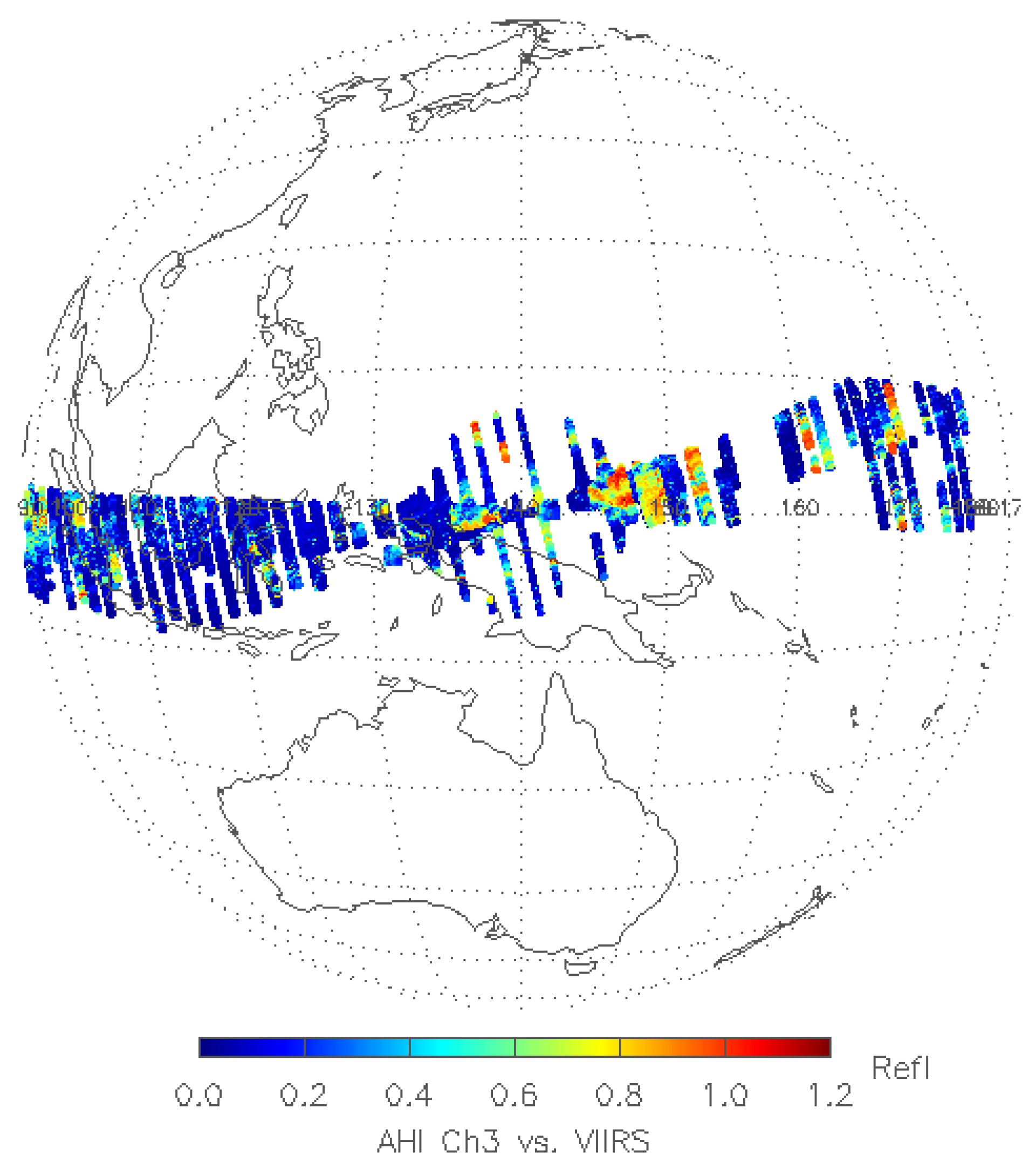
2.2. GEO-LEO Collocations

Satellite inter-comparison/inter-calibration is usually based on the comparison of measurements of the same targets. In order to reduce the uncertainty caused by impacts of atmospheric component variations and target surface BRDF, both instruments should view the geo-spatially collocated targets at similar viewing geometries within a short time interval. The following criteria are used to identify the collocated pairs without the match of viewing azimuth angles, similar to the collocation criteria applied to the GEO-LEO IR inter-calibration by the Global Satellite Inter-Calibration System (GSICS) community for the GEO-LEO IR inter-calibration [14,15].

• The time difference between GEO and LEO observations is less than 5 min. This criterion is used to reduce the impact of atmospheric variations on the Top Of Atmosphere (TOA) reflectance, as well as to ensure similar solar illumination angles to reduce the BRDF impact.
• The cosine of viewing zenith angle difference between the GEO and LEO instrument is less than 1%. As the optical path is proportional to the cosine of the viewing zenith angle, this criterion is to ensure similar optical paths for the atmospheric absorption and scattering effects, as well as similar viewing zenith angles.
• To ensure the same targets observed by the two instruments, the spatial distance between the centers of each GEO and LEO collocated pairs is less than the nominal spatial resolution of the corresponding VIIRS band, that is, 375 m for the VIIRS I bands and 750 m for the VIIRS M bands.
• To reduce the computing time, all the AHI B1, 2, 3 and 4 images are degraded to 2-km spatial resolution by averaging the radiane and reflectance at every 2 pixels x 2 pixels (for AHI B1, 2 and 4) or 4 pixels x 4 pixels (for AHI B3). To match the AHI pixel spatial size, the arrays of 3 VIIRS pixels × 3 VIIRS pixels and 7 VIIRS pixels × 7 VIIRS pixels centered at the collocated pixel are considered as the spatially collocated VIIRS scenes for the M-band and I-band data, respectively. The mean values of 3 VIRS pixels x 3 and 7 VIIRS pixels x 7 pixels are used to simulate the AHI measurements. As the clouds may be moving within the time interval, the statistical information (mean and standard deviation) of the environmental (ENV) pixels, which are three times of the AHI pixel in size, and centered at the collocated pixels, are also archived for both AHI and VIIRS data.

Again, note that no matching criterion on viewing azimuth angles is applied to these collocations yet. As shown in Figure 2, two sets of collocation data are archived from different spatial and temporal domains: (1) the collocations within 20°S < latitude < 20°N and 120.7°E < longitude < 160.7°E and during 12:00 p.m.–3:00 p.m. Satellite Local Time (SLT) from 20 July to 20 August 2015. This collocation dataset is collected near the AHI sub-satellite region around the VIIRS ascending time. This collocation data is also used for the general calibration accuracy inter-comparison described in Section 3.1, and also used to identify the collocated Deep Convective Clouds (DCC) pixels as described in Section 3.2; and (2) day-time collocations, from 9:00 a.m. SLT to 5:00 p.m. SLT, within 10°S < latitude < 10°N and 60.7°E < longitude < 220.7°E from 20 June to 20 August 2015. The latitude threshold is used because the collocations usually occur near the Equator when matching with line of sight is required. The spatial domain is within ±80° longitude from the GEO sub-satellite point used, because the maximum angle of the Earth observed from the GEO satellite is 81.3° [16]. This set of collocations is used to assess the E–W scan mirror uniformity with the similar algorithm described in Yu et al. [17], and reported in Section 3.2.

The spatial and temporal information of the collocated data of AHI and Cross-track Infrared Sounder (CrIS), a hyperspectral radiometer also onboard the S-NPP satellite, are used to reduce the pair searching time from AHI and VIIRS images. More than ten thousand collocation scenes near the AHI sub-satellite region can be obtained every day with these criteria.

3. Ray-Matching and Collocated DCC Methods

3.1. Ray-Matching Method

The Ray-matching method provides a straight-forward tool for the direct inter-comparison between GEO and LEO instruments over all-sky scenes [18]. The method is based on the comparison of the observations over the same Earth surface targets, at which point both GEO and LEO instruments scan with similar viewing and illumination angles within similar atmospheric conditions. Matching in the viewing azimuth angle between these two instruments is also applied to reduce the BRDF impact. To ensure that the same targets observed by the two instruments, the homogeneous scenes are used by filtering with the Coefficients of Variance (CoV = standard deviation/mean) of the reflectance. The homogeneous scenes are also used to compensate for the potential navigation difference between these two satellites.

• CoV(ENV)_VIIRS < 3%, CoV(ENV)_AHI < 3% and CoV(FOV)_VIIRS < 3%. FOV is the nominal spatial size (2 km) of AHI pixel used in this study, corresponding to the field-of-view (FOV) for B5 and B6.
• |φg_eo − φ_leo| < 10°

where φg_eo and φ_leo are the GEO and LEO viewing azimuth angles, respectively.

3.2. Collocated DCC Method

DCC is highly convective clouds that overshoots the tropical tropopause layer. With a distance from the ground of more than 10 km above the tropopause, DCC strongly reduces the influences of the surface and atmosphere on the TOA visible reflectance, particularly for the contributions from the molecular scattering and atmospheric water vapor absorption. At the visible spectra (e.g., 0.4 µm–1.0 µm), DCC reflectance is nearly invariant (e.g., spectral white), as the size of the ice particles of the clouds are large enough for Mie scattering and the absorption impact is negligible [19] and is considered near Lambertian when the viewing and solar zenith angles are less than 40° [20]. However, as the wavelength increases, the impact of absorption of cloud particles increases, resulting in certain variations in the reflectance. However, as DCC is selected by the GSICS community as a common calibration target to inter-calibrate visible bands, it would be also interesting to study the performance of DCC reflectance at near infrared (NIR) bands (>1.0 µm), for example AHI B5 (1.6 µm) and B6 (2.3 µm).

The DCC calibration method is a statistical method that requires sufficient DCC pixels for robust results [21,22]. As DCC is mainly distributed within the Inter-Tropical Convergence Zone (ITCZ), the spatial domain to identify DCC pixels is defined as ±20° latitude and longitude region from the GEO sub-satellite point [20]. However, although DCC reflectance is found to be stable in the long-term, some slight intra-annual variations can be observed, probably associated with the intra-annual variations of cloud physical properties [21,22]. This seasonal variation in the DCC reflectance may result in uncertainty in the absolute calibration if not properly corrected, especially at the early stage in a satellite mission’s life.

The GEO-LEO inter-calibration over the collocated DCC pairs can overcome the problem of the seasonal variation of DCC reflectance. Assessment of different satellite global data indicated that the West Pacific Ocean area has the highest frequency of DCC pixels [23]. Therefore, it is possible to identify sufficient collocated DCC pixels within the short study period. In addition to the spatial domain, further criteria, following Doelling et al. [21], are also applied to identify the DCC pixels over the collocated pairs, as described in Section 2.2. Note that no viewing azimuth matching criterion was applied to DCC selections. Each DCC pixel reflectance is corrected with the Hu et al. [24] model for BRDF correction.

• Brightness temperature (Tb) of AHI B13 (10.4 µm) and VIIRS M15 (10.7 µm) are less than 205 K. Selection of DCC pixels is sensitive to the Tb threshold [20]. Although both AHI B13 and VIIRS M15 are, in general, well-calibrated [1,12], in this study, the Tb threshold value of 205 K is applied to both instruments to reduce the possible impact of radiometric calibration difference at extremely cold DCC pixels.
• Standard deviation of Tb for VIIRS M15 FOV and ENV arrays are less than 1 K
• Standard deviation of Tb for AHI B13 ENV arrays are less than 1 K
• CoV of reflectance for VIIRS I1 FOV and ENV arrays are less than 3%
• Both the GEO and LEO viewing zenith angle (θ_v) and solar zenith angle (θ_s) should be less than 40°, that is, θ_v < 40° and θ_s < 40°

3.3. Spectral Band Adjustment Factor (SBAF)

The Scanning Imaging Absorption spectrometer for Atmospheric CHartographY (SCIAMACHY)-derived SBAFs, provided by NASA Langley, are applied to correct the SRF differences between AHI and VIIRS [25]. As NOAA employs the VIIRS Non-Government (NG) version of SRFs for the operational calibration, the linear fit SBAF, derived with NPP-VIIRS-NG SRF, are selected from the SBAF web-tools. As the spatial domain of the Ray-matching method is dominated by ocean, the all-sky tropical ocean SBAF values are chosen in this study.

Table 2. SBAF (AHI/VIIRS) coefficients (slope and offset) for AHI VNIR bands and the uncertainty values.

SBAF	AHI	B1	B2	B3	B4		B5		B6
	VIIRS	M3	M3	I1	M7	I2	M10	I3	M11
Ray-matching (all-sky tropical Ocean)	SBAF_Slope	0.991	1.005	1.000	0.998	0.998	1.019	1.022	1.0
	SBAF_Offset	9.5e−3	−1.341e−2	–2.07e−4	−4.18e−4	−3.67e−4	−2.216e−4	−2.465e−4	0.0
	Uncertainty (%)	0.820	1.172	0.187	0.448	0.422	1.701	1.839	-
Coll. DCC	SBAF_Slope	0.992	1.014	1.000	1.003	1.003	1.035	1.038	1.0
	SBAF_Offset	9.989e−3	−2.124e−2	1.594e−5	−1.545e−3	−1.459e−3	2.472e−3	2.875e−3	0.0
	Uncertainty (%)	0.238	0.596	0.033	0.106	0.100	0.736	0.753	-

lists the SBAF coefficients and their uncertainties from the web-tools. Unfortunately, there is no SCIAMACHY-based SBAFs for AHI B6 (2.3 µm). We assume that the SBAF for this band is 1.0 due to the similar SRFs between AHI B6 and VIIRS M11, and there is no strong absorption within the spectral range (Figure 1). In this study, all the inter-calibration analyses are based on reflectance. All the AHI data used for inter-comparison with VIIRS are corrected with SBAF coefficients as follows:

$$R_{VIIRS,AHI}=(R_{AHI}-SBAF\_Offset)/SBAF\_Slope$$

(1)

where R_AHI is the AHI reflectance and R_VIIRS,AHI is the corresponding AHI reflectance corrected with VIIRS SRF. SBAF_Slope and SBAF_Offset are the slope and offset of the SCIAMACHY-based linear regression coefficients, respectively.

4. Results and Discussions

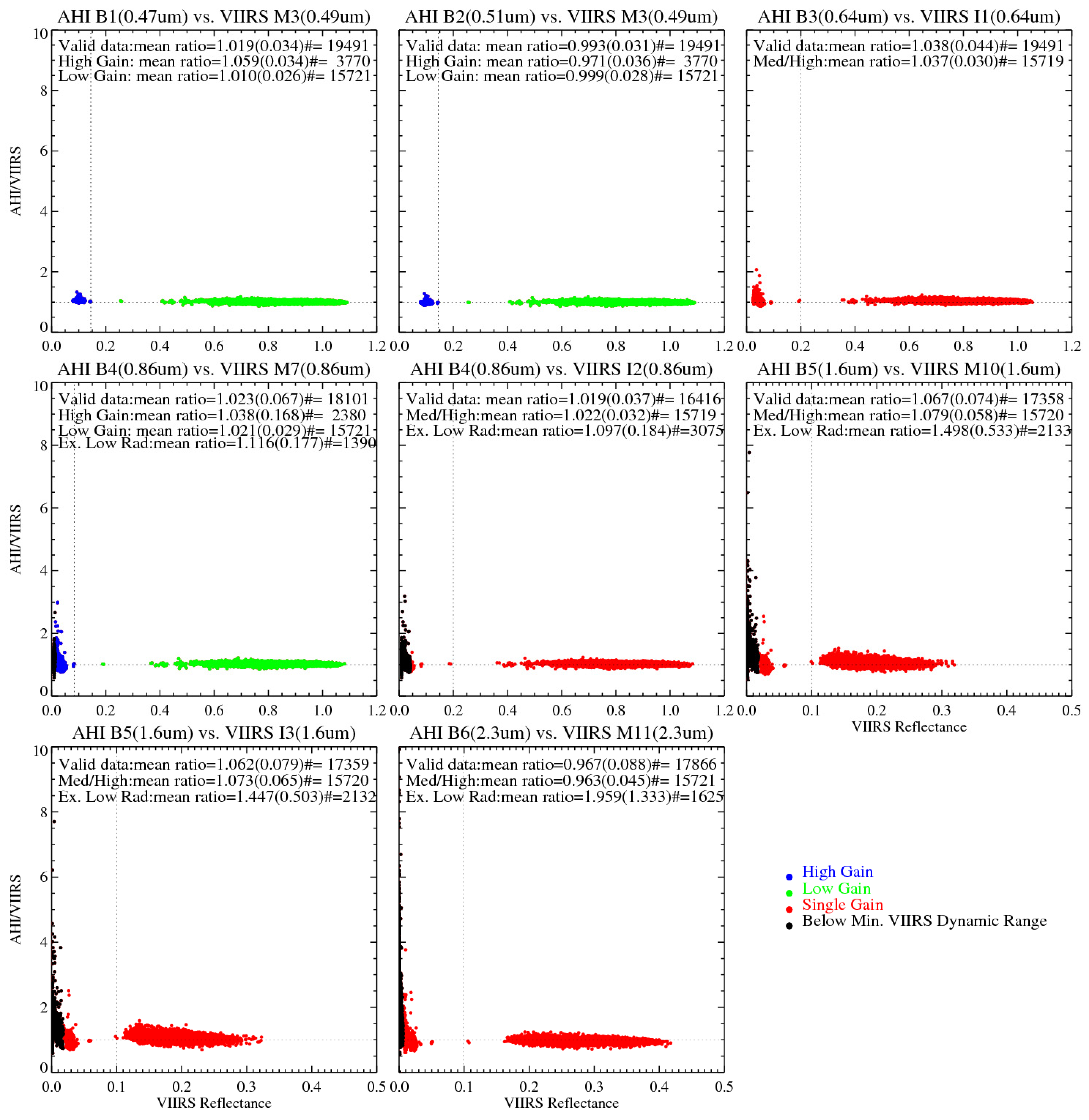
4.1. Ray-Matching Inter-Calibration: Large Measured Radiance/Reflectance Range

Figure 3 are the scatter-plots of AHI and VIIRS reflectance from the homogeneous scenes selected with the Ray-matching method. To avoid directional reflectance from the sun-glint area caused by the specular reflection, only collocations beyond the sun-glint angle of 25° (ƞ > 25), which is selected to balance the requirements of sufficient collocation for analysis and, meanwhile, to reduce the sun-glint impact, are used for this analysis. The sun-glint angle is calculated with the following equation [26]:

$$\cos (\eta )=\cos ({\theta }_s)\cos ({\theta }_v)+\sin ({\theta }_s)\sin ({\theta }_v)\cos (180-\phi )$$

where ƞ is the sun glint angle, θ_s and θ_v are the solar zenith angle and satellite viewing zenith angle, respectively, and φ is the relative azimuth angle between solar and viewing azimuths.

As shown in Figure 3, there are strong linear relationships between the AHI reflectance and the corresponding VIIRS M and I data. Two of VIIRS M bands used in this study, M3 and M7, have dual gain design. Although the homogenous criteria removes most scenes at a median-radiance level when they are partially covered with cloud, the selected scenes still cover large radiance ranges from the low radiance of clear ocean scenes to the high reflectance of cloud covered or bright scenes. The offsets of the linear fitting functions are very small and positive, less than 0.6% for AHI B3-6. Due to the Rayleigh scattering of which effect on the TOA radiance or reflectance decreases with an increase in wavelength, the minimum reflectance values are about 7.8% and 2.5% for VIIRS M3 and I1, respectively, and about 9.1%, 6.4% and 2.4% for AHI B1, B2 and B3, respectively. It is also expected that AHI B2 reflectance of clear ocean scenes should be smaller than VIIRS M3 as the AHI B2 central wavelength is larger than that of VIIRS M3. However, the fitting slope of the collocated scenes at M3 high-gain data is 1.2 (AHI is generally bright than VIIRS), while the slope of scenes at the low-gain part is 0.97 (AHI is generally darker than VIIRS). The discrepancy of the fitting slopes at high-gain and low-gain data may suggest that the SCIAMACHY-based Ray-matching SBAF has some uncertainty for the clear-sky open ocean data for this pairs of instrument bands. Two possible reasons can be attributed to the SBAF uncertainty: (1) the large SRF difference between AHI B2 and VIIRS M3, and (2) the large foot-print of SCIAMACHY made it hard to find clear sky ocean pixels in the low radiance end pixels.

The collocated data in the figure are classified with VIIRS specification values: the high gain and low gain switchover radiace and the minimum values of dynamic ranges. Due to the stringent requirements from the user community, the minimums of dynamic ranges are specified at VIIRS VNIR bands and used to generate meaningful physical products. Some extremely low VIIRS radiance scenes with a mean FOV radiance below the minimum of the VIIRS dynamic range values can be observed at the bands of M7, M10, M11, I2 and I3. These are most likely very clean ocean surface scenes, from which the signals reaching the instrument’s aperture are very small at these bands. For the two short-wave bands (M3 and I1), the effect of Rayleigh scattering increases the TOA reflectance and, thus, all the radiance at the two bands are larger than the minimum specifications. There is no minimum dynamic range specification for AHI data [27].

The calibration difference between these two instruments can be displayed with the scene dependent reflectance ratios (ratio = AHI/VIIRS) (Figure 4). All the paired bands display relatively large variation in the reflectance ratio at the low radiance scenes, while the ratio is relatively consistent at median and high radiance ones. The most likely reason is that impact of noises is most apparent at low radiance scenes. Thus the outliers, which have the VIIRS radiance less than the minimum of VIIRS dynamic range, display the largest variations in the ratios. Several reasons may cause the relatively large variation in the reflectance ratio at low reflectance scenes. One possible source could be the small AHI instrument coherent noise, as the magnitude of ratios increases with the central wavelength from visible to NIR bands, while the reflected solar energy decreases at these bands (Figure 4). Like ABI, AHI also applies a resampling algorithm in generating the fixed grid L1B data [28]. According to Pgorzala et al. [29], the resampling process has the potential to both smooth and amplify the radiance variations within the neighouring samples [29]. In this study, although the CoV values of AHI and VIIRS ENV arrays’ reflectance are applied to ensure the homogeneous collocations, the resampling process may cause deviation of the collocated AHI reflectance and, thus, be attributed to the ratio variation. Slight difference in detector-to-detector responsivity may also contribute to the ratio variations. Another possible noise source is the different directional reflectance resulting from the movement of sun-glint mask residual, if any, within the collocation time interval. Additionally, interestingly, at the VIIRS dual-gain bands (M3 and M7), there is no homogeneous collocation available at the low-gain side near the switchover point between high and low gains [5,8]. Further effort is needed to understand the causes of these ratio variations at the VIIRS high gain or low radiance scenes.

As shown in Figure 4, the median/high reflectance scenes have relatively consistent reflectance ratios. A set of radiance and reflectance thresholds are then used to separate the median/high radiance scenes from the low radiance scenes to further analyze the AHI and VIIRS calibration differences. For the VIIRS dual-gain bands (M3 and M7), the radiance values of the switchover points are used as the threshold to define the median/high radiance scenes. A reflectance value of 0.2 for AHI B3 and B4 and reflectance of 0.1 for AHI B5 and B6 are used as thresholds. The mean and standard deviation of the reflectance ratios from the median/high collocated scenes are reported in

Table 3. Reflectance ratio between AHI and VIIRS M and I bands for the ray-matched median/high reflectance scenes and collocated DCC measurements.

AHI		B1	B2	B3	B4		B5		B6
VIIRS		M3	M3	I1	M7	I2	M10	I3	M11
Ray-matching		1.010 (±0.026)	0.999 (±0.028)	1.037 (±0.030)	1.021 (±0.029)	1.022 (±0.032)	1.079 (±0.058)	1.073 (±0.065)	0.963 (±0.045)
DCC	Median	1.002	0.992	1.031	1.014	1.015	1.067	1.061	0.955
	Mode	0.992	0.985	1.030	1.024	1.014	1.102	1.084	0.977
	Mean	1.003	0.994	1.031	1.014	1.015	1.064	1.058	0.958
	Statistics *	1.003 (±0.024)	0.995 (±0.026)	1.032 (±0.028)	1.015 (±0.024)	1.015 (0.025)	1.065 (±0.030)	1.059 (±0.032)	0.959 (±0.026)

*: mean and standard deviation of the reflectance ratios for all the collocated DCC scenes at each paired bands.

. As shown in this table, AHI radiometric calibration accuracy agrees well with that of VIIRS, within a 5% difference, except for B5: AHI reflectance is generally higher than VIIRS data at B1, B3, and B4 by 1.0%, 3.7%, and 2.1%, respectively, and lower than VIIRS data at B2 by 0.1% and B6 by 3.7%. The largest reflectance difference occurs at AHI B5, which is, in general, larger than VIIRS M10 and I3 data by 7%–8%. Similar results between the AHI and VIIRS inter-calibration were also reported by JMA with the Ray-matching method [1].

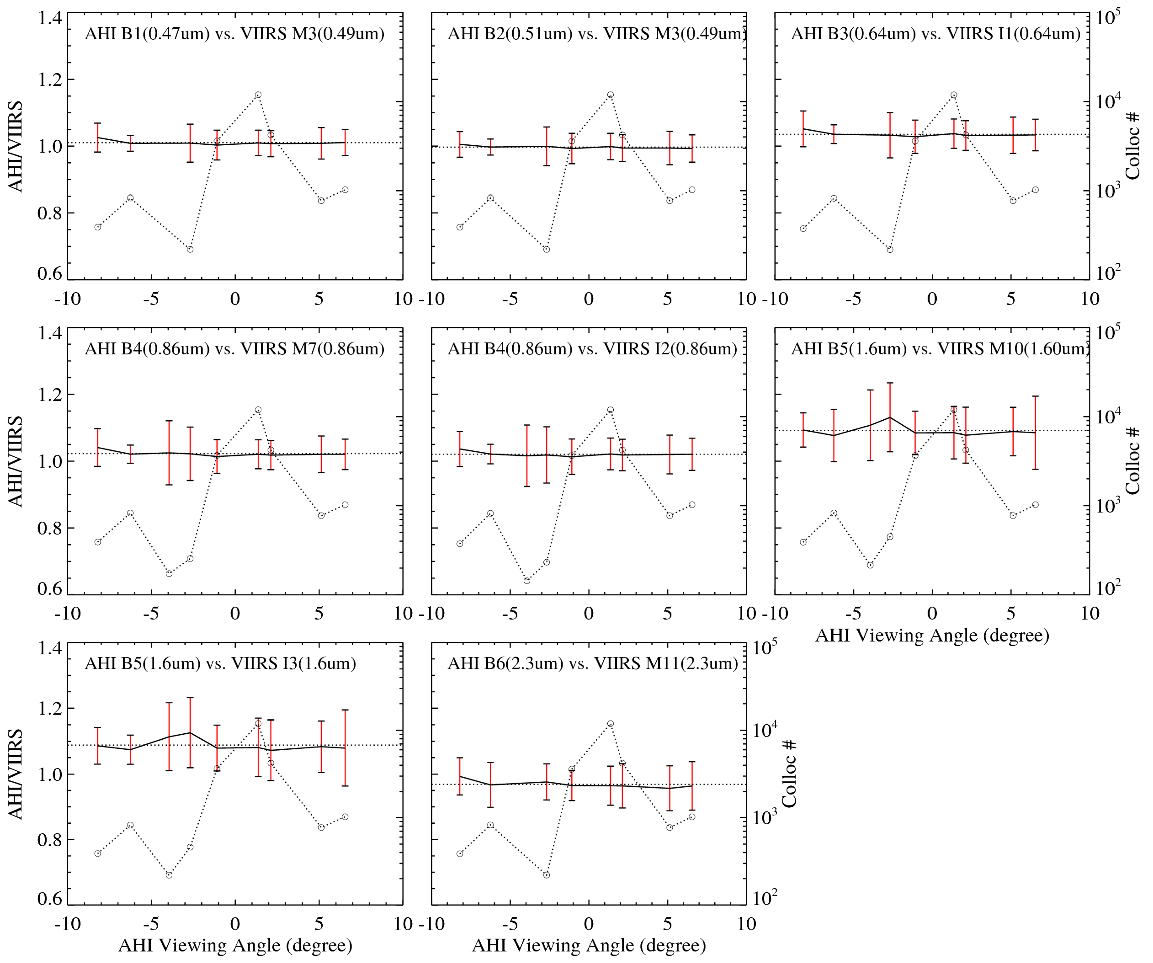
4.2. Ray-Matching Inter-Calibration: E–W Viewing Angle Dependent Calibration Difference

Figure 5 shows the spatial distribution of the Ray-matched collocations within 10°S to 10°N from 20 June to 20 August 2015. Due to the inclination of S-NPP (98.69°), the collocations east of the GEO nadir are mainly distributed in the Northern hemisphere, while those west of the sub-satellite points are mainly in the Southern hemisphere. Such a wide distribution of the Ray-matched collocations along the Equator, thus, provides an opportunity to examine the viewing angle dependent calibration difference between these two satellites. This assessment is applied to the homogenous median/high reflectance scenes. No mask of sun-glint area is applied because the sun-glint effects on the median/high reflectance scenes are statistically very small. This is because clouds usually do not have strong directional forward or backward reflectances as those of clear ocean surfaces [30].

According to the GEO satellite and Earth geometry, the maximum viewing angle from the GEO satellite to the Earth surface is 8.7° [14]. The viewing angle is defined as the angle between the sub-satellite point, GEO satellite and the viewing target on the Earth. The collocation data are equally split into 10 bins between −8.7° and +8.7°. The AHI pixel coordinates are used to calculate the viewing angle. For the AHI pixels at 2 km normal spatial resolution, the Instantaneous Geometric Field of View (IGFOV) is 56 µrad. A minimum of 100 homogeneous scenes is required to calculate the mean and standard variation values of reflectance ratio at each valid bin. The angular dependent reflectance ratios for each AHI and corresponding VIIRS bands are shown in Figure 6. No apparent trending can be observed at these bands with a GEO viewing angle of <7°, which is less than about 50° of GEO and LEO viewing zenith angles. Relatively large ratio variations can be observed at a few viewing angle bins of AHI B5, but they are associated with relatively larger uncertainty. Slight positive deviation can be observed at AHI B1 vs. M3, B3 vs. I1, B4 vs. M7, B4 vs. I2, and B6 vs. M11 for the data with AHI viewing zenith angle less than −7° (about 50° for the GEO and LEO viewing zenith angles, west of the nadir point). However, the deviations are within the measurement uncertainty level. Unfortunately, no collocation data are selected for viewing angles larger than 7° in this study. Extension of AHI and VIIRS collocation time threshold earlier than 9:00 a.m. SLT should be applied to cover the viewing angles in future studies. Unfortunately, a large portion of the collocations had low reflectance during this study period (Figure 5), a longer period or a different study period will be needed to ensure robust results with sufficient median/high reflectance numbers for all the viewing angle bins.

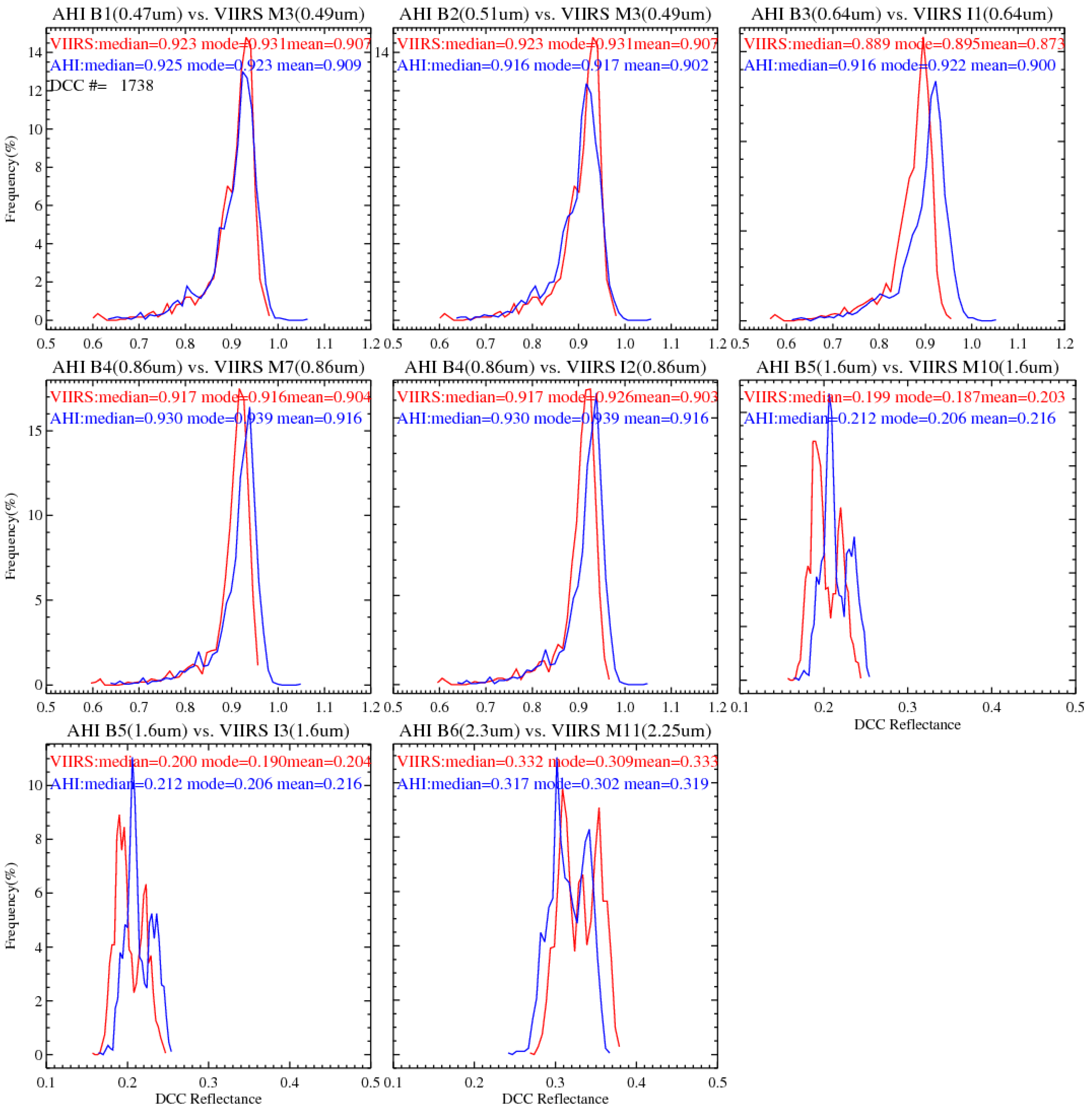
4.3. Collocated DCC Results

The DCC pixels are selected with AHI B3 and B13, and VIIRS I1 and M15 measurements (Figure 2). About 2500 collocated DCC pixels are identified during the study period, from 20 July to 20 August 2015. Figure 7 shows the histograms of the DCC reflectances. Each pair of AHI and VIIRS data exhibit very similar but shifted histogram shapes. While the DCC shows single mode and high reflectance at the bands with wavelength less than 1.0 µm (AHI B1-4 and VIIRS M3, M7, I1 and I2), the reflectance is relatively low with bi-model histogram patterns at 1.6 µm (AHI B5 and VIIRS M10 and I3) and 2.3 µm (AHI B6 and VIIRS M11). The VIIRS DCC data at all the short-wavelength bands display sharper-shaped histograms than the corresponding AHI data. This is because AHI has wider dynamic ranges than VIIRS at these visible bands with less quantization bits [8,26]. While the VIIRS data are truncated to 12 bits, AHI data are truncated to 11 bits. The narrower dynamic range and more quantization bits make VIIRS data more sensitive to the slight variations of DCC reflectance, which are believed to be statistically very stable at the visible wavelength.

Three types of DCC measurements are used to represent the DCC reflectance: median, mode and mean values of the DCC data. Therefore, in addition to the statistics of each DCC pair, there are four methods to calculate the reflectance ratios of DCC of these two instruments. As reported in Table 3, the results of the four types of reflectance ratios agree very well with those derived from the Ray-matching method: the calibration differences between AHI and VIIRS are less than 5% for AHI B1-4 and B6, however, AHI B5 is brighter than VIIRS by about 6%–8%. Although DCC is not among the brightest Earth targets at the NIR bands, the collocated DCC method provides less uncertainty for the GEO-LEO inter-calibration than the Ray-matching method. For the visible wavelength bands (<1.0 µm), collocated DCC have very comparable inter-calibration uncertainty with the Ray-matching method. Due to the existence of bi-model reflectance histograms, the median or mean value of DCC reflectance may be considered for long-term trending of calibration accuracy for these two NIR bands. Further study is needed to understand the causes to the bi-mode pattern.

5. Conclusions

Both AHI and VIIRS use a solar diffuser as a bright target to provide on-orbit calibration for the VNIR bands. In this study, two inter-calibration methods are used to compare the AHI VNIR radiometric calibration accuracy with the collocated VIIRS measurements for the six AHI VNIR bands. These two methods are based on spatially collocated pairs, which the two instruments view with the same viewing zenith angles within a 5 min difference. The Ray-matching method uses collocated homogeneous scenes with similar viewing azimuth angles, while the collocated DCC method uses the near-Lambertion effect of the DCC pixels. Therefore, the Ray-matching method can provide inter-calibration results for all sky scenes, while the collocated DCC method focuses on the calibration differences at median or high reflectance pixels. Viewing angle dependent calibration difference at homogenous median/high reflectance scenes is also examined with the Ray-matching method.

The Ray-matching method shows there is a strong linear relationship between AHI and VIIRS at all the paired bands. Results of both the Ray-matching and collocated DCC methods indicate that AHI radiance quality agrees well with that of VIIRS, within a 5% difference, except for AHI B5, which is brighter than VIIRS M10 and I3 by 6%–8%. Relatively larger reflectance ratio variation, which increases with wavelength, can be observed at low radiance scenes, probably associated with certain AHI instrument noises. No trending in the E–W viewing angular dependent calibration difference between these two instruments can be observed within the uncertainty of the Ray-matching method.

The good agreement of the inter-calibration results between the Ray-matching and collocated DCC methods for all the paired bands indicate that the DCC method can also be used for the calibration of NIR bands. Compared to the Ray-matching method, the collocated DCC method has less uncertainty on the inter-calibration results for the NIR bands. Further study may be needed to understand the bi-mode patterns of the NIR DCC reflectance histograms. Overall, the earlier launch of AHI provides a unique opportunity to develop, test and examine the ABI cal/val tools.

References

1. Takahashi, M.; Andou, A.; Date, K.; Hosaka, K.; Mori, N.; Murata, H.; Okuyama, A.; Tabata, T.; Yoshino, R.; Bessho, K. Himawari-8 post-launch radiometric calibration and navigation analysis. In Proceedings of the 2015 EUMETSAT Conference, Toulouse, France, 21–25 September 2015.
2. Cao, C. Overview and progress update on GOES-R calibration/validation. In Proceedings of the 2012 AMS 92nd Annual Meeting/8th Annual Symposium on Future Operational Environment Satellite System, New Orleans, LA, USA, 22–26 January 2012.
3. Pearlman, A.; Pogorzala, D.; Cao, C. GOES-R Advanced Baseline Imager: Spectral functions and radiometric biases with the NPP visible infrared imaging radiometer suite evaluated for desert calibration sites. Appl. Opt. 2013, 31, 7660–7668. [Google Scholar] [CrossRef] [PubMed]
4. Xiong, J.; Butler, J.; Chiang, K.; Efremova, B.; Fulbright, J.; Lei, N.; McIntire, J.; Oudrari, H.; Sun, J.; Wang, Z.; et al. VIIRS on-orbit calibration methodology and performance. J. Geophys. Res.: Atmos. 2013, 118, 5065–5078. [Google Scholar] [CrossRef]
5. Cao, C.; Xiong, X.; Blonski, S.; Liu, Q.; Uprety, S.; Shao, X.; Bai, Y.; Weng, F. Suomi NPP VIIRS sensor data record verification, validation, and long-term performance monitoring. J. Geophys. Res.: Atmos. 2013, 118, 1–15. [Google Scholar] [CrossRef]
6. Uprety, S.; Cao, C. Suomi NPP VIIRS reflective solar band on-orbit radiometric stability and accuracy assessment using desert and Antarctica Dome C sites. Remote Sens. Environ. 2015, 166, 106–115. [Google Scholar] [CrossRef]
7. Griffith, C. ABI’s unique calibration and validation capabilities. In Proceedings of the 2015 EUMETSAT Conference, Toulouse, France, 21–25 September 2015.
8. NOAA/STAR VIIRS SDR Team and the science team members. Joint Polar Satellite System (JPSS) Visible Infrared Imaging Radiometer Suite (VIIRS) Sensor Data Records (SDR) Radiometric Calibration Algorithm Theoretical Basis Document (ATBD) 2013. Available online: http://www.star.nesdis.noaa.gov/smcd/spb/nsun/snpp/VIIRS/ATBD-VIIRS-RadiometricCal_20131212.pdf (accessed on 19 November 2015).
9. McIntire, J.; Moyer, D.; Efremova, B.; Oudrari, H.; Xiong, X. On-orbit characterization of S-NPP VIIRS transmission functions. IEEE Trans. Geosci. Remote Sens. 2015, 53. [Google Scholar] [CrossRef]
10. Bessho, K.; Date, K.; Hayashi, M.; Ikeda, A.; Imai, T.; Inoue, H.; Kumagai, Y.; Miyakawa, T.; Murata, H.; Ohno, T.; et al. An introduction to Himawari-8/9—Japan’s new-generation geostationary meteorological satellites. J. Meteorol. Soc. Jpn. 2016. [Google Scholar] [CrossRef]
11. Japan Meteorological Agency (JMA) Himawari-8 Advanced Himawari Imaer (AHI) Webpage. Available online: http://www.data.jma.go.jp/mscweb/en/himawari89/space_segment/spsg_ahi.html (accessed on 19 November 2015).
12. Cao, C.; de Luccia, F.; Xiong, X.; Wolfe, R.; Weng, F. Early on-orbit performance of the visible infrared imaging radiometer suite onboard the Suomi National Polar-Orbiting Partnership (S-NPP) satellite. IEEE Trans. Geosci. Remote Sens. 2014, 52, 1142–1156. [Google Scholar] [CrossRef]
13. Wolfe, R.; Lin, G.; Nishihama, M.; Tewari, K.; Tilton, J.; Isaacman, A. Suomi NPP VIIRS prelaunch and on-orbit geometric calibration and characterization. J. Geophys. Res. 2013, 118, 11508–11521. [Google Scholar]
14. Wu, X.; Hewison, T.; Tahara, Y. GSICS GEO-LEO inter-calibration: Baseline algorithm and early results. Proc. SPIE 2009, 7456. [Google Scholar] [CrossRef]
15. Hewison, T.; Wu., X.; Yu, F.; Tahara, Y.; Hu, X.; Kim, D.; Koenig, M. GSICS inter-calibration of infrared channels of geostationary imagers using Metop/IASI. IEEE Trans. Geosci. Remote Sens. 2013, 51, 1160–1170. [Google Scholar] [CrossRef]
16. Gardashov, R.; Eminov, M. Determination of sunglint location and its characteristics on observation from a METEOSAT 9 satellite. Int. J. Remote Sens. 2015, 36, 2584–2598. [Google Scholar] [CrossRef]
17. Yu, F.; Wu, X.; Varma Raja, M.; Li, Y.; Wang, L.; Goldberg, M. Diurnal and scan angle variations in the calibration of GOES Imager infrared channels. IEEE Trans. Geosci. Remote Sens. 2013, 51, 671–683. [Google Scholar] [CrossRef]
18. Doelling, D.; Minnis, P.; Nguyen, L. Calibration comparison between SEVERI, MODIS and GOES data. In Proceedings of the 2004 MSG RAO Workshop, Salzburg, Austria, 6–10 September 2004.
19. Sohn, B.-J.; Ham, S.; Yang, P. Possibility of the visible-channel calibration using deep convective clouds overshooting the TTL. J. Appl. Meteorol. Climatol. 2009, 48, 2271–2283. [Google Scholar]
20. Doelling, D.; Nguyen, L.; Minnis, P. On the use of deep convective clouds to calibrate AVHRR data. SPIE Proc. 2004, 5542. [Google Scholar] [CrossRef]
21. Doelling, D.; Morstad, D.; Scarino, B.; Bhatt, R.; Gopalan, A. The characterization of deep convective clouds as an invariant calibration target and as a visible calibration technique. IEEE Trans. Geosci. Remote Sens. 2013, 51, 1147–1159. [Google Scholar] [CrossRef]
22. Yu, F.; Wu, X. An integrated method to improve the GOES Imager visible radiometric calibration accuracy. Remote Sens. Environ. 2015, 164, 103–113. [Google Scholar] [CrossRef]
23. Beuchler, D.; Koshak, W.; Christian, H.; Goodman, S. Assessing the performance of the Lightning Imaging Sensor (LIS) using deep convective clouds. Atmos. Res. 2014, 135–136, 397–403. [Google Scholar] [CrossRef]
24. Hu, Y.; Wielicki, B.; Yang, P.; Stackhouse, P.; Lin, B.; Young, D. Application of deep convective cloud albedo observation to satellite-based study of terrestrial atmosphere: Monitoring the stability of spaceborn measurement and assessing absorption anomaly. IEEE Trans. Geosci. Remote Sens. 2004, 42, 2594–2599. [Google Scholar]
25. Scarino, B.; Doelling, D.; Minnis, P.; Gopalan, A.; Chee, T.; Bhatt, R.; Lukashin, C.; Haney, C. A web-based tool for calculating spectral band difference adjustment factors derived from SCIAMACHY hyper-spectral data. IEEE Trans. Geosci. Remote Sens. 2016. [Google Scholar] [CrossRef]
26. NOAA/NESDIS/STAR, Algorithm Theoretical Basis Document, ABI Aerosol Detection Product, May 2010. Available online: http://www.star.nesdis.noaa.gov/goesr/docs/ATBD/ADP.pdf (accessed on 19 November 2015).
27. Japan Meteorological Agency. AHI-8 Performance Test Results, 2015. Available online: http://www.data.jma.go.jp/mscweb/en/himawari89/space_segment/doc/AHI8_performance_test_en.pdf (accessed on 19 November 2015).
28. Okuyama, A.; (Japan Meterological Agency, Tokoyo, Japan). Personal communication, 2014.
29. Pogorzala, D.; Padula, F.; Cao, C.; Wu, X. The GOES-R ABI fixed format: Overview and case sudy. Available online: http://adsabs.harvard.edu/abs/2014AGUFMIN43C3702P (accessed on 19 November 2015).
30. Zuidema, P.; Davies, R.; Moroney, C. On the angular radiance closure of tropical cumulus cognestus clouds observed by the Multiangle Imaging Spectroradiometr. J. Geophys. Res. 2003, 108, 4626–4637. [Google Scholar] [CrossRef]
Figure 1. Spectral response function (SRF) of AHI (black) and VIIRS (red for M bands and in blue for I bands), as well as the atmospheric transmission (gray shadow), and vegetation and water spectra (dark, dashed lines). The VIIRS SRFs plotted are of Non-Government (NG) version [6].
Remotesensing 08 00165 g001
Figure 2. Flow-chart of AHI vs. VIIRS inter-calibration processes. The time and spatial location information of AHI and CrIS collocations are used to restrict the temporal and spatial searching domains. θgeo and θleo are the GEO and LEO viewing zenith angles, respectively. φgeo and φleo are the viewing azimuth angles for GEO and LEO instruments, respectively. ƞ is the sun-glint angle.
Remotesensing 08 00165 g002
Figure 3. Relationship between homogeneous ray-matched AHI and VIIRS data from 20 July to 20 August 2015. The x-axis is VIIRS reflectance and y-axis is AHI reflectance.
Remotesensing 08 00165 g003
Figure 4. Scene dependent reflectance ratio for the homogeneous ray-matched AHI and VIIRS collocations from 20 July to 20 August 2016. The x-axis is the VIIRS reflectance and y-axis is AHI and VIIRS reflectance ratio. The vertical dashed lines are the thresholds used to separate the median/high radiance scenes from the low radiance ones. The horizontal dashed line is the ratio of 1.0. The outliers are the collocations with VIIRS radiance less than the VIIRS minimum dynamic ranges.
Remotesensing 08 00165 g004
Figure 5. Spatial distribution of Ray-matched collocations within ±10° latitude for the collocation data collocated from 20 June to 20 August 2015.
Remotesensing 08 00165 g005
Figure 6. The E–W viewing angle dependent reflectance ratio between AHI and VIIRS for the data collected from 20 June to 20 August 2015. The red segments represent the standard deviation of the reflectance ratio at each valid bin. The open circles connected with dashed lines are the number of selected scenes and are referred with the second y-axis which ranges from 102 to 105. The x-axis is AHI viewing angle in degree.
Remotesensing 08 00165 g006
Figure 7. Histograms of collocated DCC reflectance for the data collected from 20 July to 20 August 2015, All the bands have the same DCC pixels. The y-axis is the DCC frequency (%) and the x-axis is the DCC reflectance.
Remotesensing 08 00165 g007