Article

Validation and Spatiotemporal Analysis of CERES Surface Net Radiation Product

1
State Key Laboratory of Remote Sensing Science, and School of Geography, Beijing Normal University, Beijing 100875, China
2
Department of Geographical Sciences, University of Maryland, College Park, MD 20742, USA
*
Author to whom correspondence should be addressed.
Remote Sens. 2016, 8(2), 90; https://doi.org/10.3390/rs8020090
Submission received: 12 October 2015 / Revised: 19 December 2015 / Accepted: 18 January 2016 / Published: 23 January 2016

Abstract

:
The Clouds and the Earth’s Radiant Energy System (CERES) generates one of the few global satellite radiation products. The CERES ARM Validation Experiment (CAVE) has been providing long-term in situ observations for the validation of the CERES products. However, the number of these sites is low and their distribution is globally sparse, and particularly the surface net radiation product has not been rigorously validated yet. Therefore, additional validation efforts are highly required to determine the accuracy of the CERES radiation products. In this study, global land surface measurements were comprehensively collected for use in the validation of the CERES net radiation (Rn) product on a daily (340 sites) and a monthly (260 sites) basis, respectively. The validation results demonstrated that the CERES Rn product was, overall, highly accurate. The daily validations had a Mean Bias Error (MBE) of 3.43 W·m−2, Root Mean Square Error (RMSE) of 33.56 W·m−2, and R2 of 0.79, and the monthly validations had an MBE of 3.40 W·m−2, RMSE of 25.57 W·m−2, and R2 of 0.84. The accuracy was slightly lower for the high latitudes. Following the validation, the monthly CERES Rn product, from March 2000 to July 2014, was used for a further analysis. The global spatiotemporal variation of the Rn, which occurred during the measurement period, was analyzed. In addition, two hot spot regions, the southern Great Plains and south-central Africa, were then selected for use in determining the driving factors or attribution of the Rn variation. We determined that Rn over the southern Great Plains decreased by −0.33 W·m−2 per year, which was mainly driven by changes in surface green vegetation and precipitation. In south-central Africa, Rn decreased at a rate of −0.63 W·m−2 per year, the major driving factor of which was surface green vegetation.

Graphical Abstract

1. Introduction

The surface radiation budget (SRB) plays an important role in hydrological and biological modeling, and agricultural science and its applications [1,2]. The SRB components consist of the downward shortwave irradiance (DSW), upward shortwave irradiance (USW), downward longwave flux (DLW), upward longwave flux (ULW), and net all-wave radiation (Rn). The surface Rn is the sum of the four formerly-mentioned radiation components, and can be represented mathematically:
R n = R s R s + R l R l
where Rs denotes the DSW (W·m−2), Rs denotes the USW (W·m−2), Rl denotes the DLW (W·m−2), and Rl denotes the ULW (W·m−2).
The surface Rn can be obtained by ground observation stations, general circulation model (GCM) simulations, and remote sensing retrieval [3]. Comparatively, in situ observations have the highest accuracy; however, they are very expensive to measure at ground sites. Additionally, these ground sites are sparsely distributed, globally, and cannot meet the requirements of various applications. Data simulated by GCMs usually have a coarse spatial resolution and low accuracy [2]. Remote sensing retrieval has become one of the most important methods for obtaining the radiation data [4]. However, clouds make it impossible to retrieve surface thermal radiation components directly from satellite observations, and the alternative solution is to estimate the all-wave net radiation from the satellite shortwave net radiation product, in conjunction with other information [5,6].
The CERES surface net radiation data are calculated using the radiative transfer model, with the atmospheric and surface properties obtained from a variety of sources used as the model inputs, but constrained by both solar-reflected and Earth-emitted radiation from the top of the atmosphere (TOA) for all-sky and clear-sky conditions [7]. Charlock et al. [8] conducted the CERES/ARM/GEWEX Experiment (CAGEX) before the launch of satellites, in order to validate the Fu-Liou radiative transfer model [9]. They found that the modeled longwave radiation agrees well with the in situ observations, while the shortwave radiation exhibits a large difference between the modeled and in situ data. Since then, CAGEX has been developed to become the CERES ARM Validation Experiment (CAVE) [10], which provides validation data and model parameters, which are measured on the ground for each version of the CERES radiation product. It includes 84 sites, with limited spatial distribution [11]. David Rutan et al. [12] utilized 40 sites in order to validate the Clouds and Radiative Swath (CRS), and found that the RMSEs were related to the land cover type. Gui et al. [13] validated the CERES- Monthly Gridded Radiative Fluxes and Clouds (FSW) in the Tibetan Plateau, and found that the CERES had a lower accuracy for shortwave radiation. Wang et al. [14] also found that FLASHFlux/CERES (Fast Longwave and Shortwave Fluxes Time Interpolated and Spatially Averaged/CERES) satellite products over rugged terrains showed absolute errors of about 31.4 W·m−2 (12.3%). Pan et al. [15] assessed the CERES Rn product by using 50 ground sites in China, and showed that 56% of the net radiation errors come from the net shortwave radiation. Kratz et al. [16] validated the CERES_Ed2b algorithms, and found that the shortwave radiation had systematic errors of approximately 14–21 W·m−2, which does not meet the meteorological research. In addition, the CERES Ocean Validation Experiment (COVE) [17] has been collecting data for the validation of CERES on the sea using one site. Charlock et al. [18] validated the CERES data on the sea in 2001, using the Chesapeake Lighthouse and Aircraft Measurements for Satellites (CLAMS) and COVE data, and the results were good. However, all of these previous studies into the validation of the CERES had a low number and distribution of sites, and the accuracies of the CERES Rn around the global land surface are still generally unknown. Therefore, the CERES surface net radiation product needs to be validated globally.
Wild et al. [19] obtained a global Rn mean value from 2000 to 2004 by calculating the best estimation of shortwave and longwave radiation over the land surface and oceans utilizing 43 Coupled Model Intercomparison Project Phase 5 (CMIP5) model datasets. Sobrino et al. [20] researched the DSW and Rn around the globe from 1980 to 2010 by using National Centers for Environmental Prediction (NCEP) and the National Center of Atmospheric Research (NCAR) re-analysis data and detected a decrease in these values in selected areas. Gao et al. [21] detected a decrease in Rn over China by using the 1961–2010 data of 699 meteorological stations. Shi et al. [22] fused several radiation data and analyzed the spatiotemporal variation of SRB over the Tibetan Plateau in the past 30 years. However, these previous studies on Rn variation were based mainly on data with high uncertainties, and some research focused only on partial areas. Therefore, global spatiotemporal analysis of Rn utilizing data with high accuracy is urgently needed.
In this study, the measurements obtained from observation sites around the world were collected to be used for validating the CERES_SYN1deg_Ed3A Rn product under all-sky conditions on a daily (340 sites) and a monthly (260 sites) basis, respectively. Considering that most Rn variation studies were mainly developed in limited areas and the chosen radiation data had high uncertainties, the CERES monthly Rn product, from March 2000 to July 2014, was used for a further spatiotemporal analysis across the global land surface. As the southern Great Plains and south-central Africa are located in special and vital geographical locations, they were chosen as hot spots for a detailed analysis of the relationship between the variations in surface Rn and their driving factors.
This paper proceeds as follows: the CERES, in situ observations, driving factor datasets, and experiment methods are introduced in Section 2; the validation and spatiotemporal analysis results and discussions are shown in Section 3; and the conclusions are provided in Section 4.

2. Data and Methods

2.1. Data

2.1.1. The CERES Data

The CERES_SYN1deg_Ed3A product is used in this study. The “SYN” (Synoptic Radiative Fluxes and Clouds) means that this version provides radiation data on clear and all sky conditions, the ”1deg” means it has a 1 degree spatial resolution, and the “Ed3A” is the version number [23]. In addition to the radiation flux, this version also provides MODIS cloud properties and aerosols information. As the three-hourly sampled geostationary (GEO) radiances and cloud properties were used to model the diurnal variability between observations, this version achieves more accurate retrieval results than previous versions [24]. The CERES consists of three-hourly, daily, and monthly data, released on Greenwich Mean Time (GMT) [25]. The data we used ranged from 1 March 2000 to 30 July 2014. In this study, three-hourly and monthly DSW, USW, DLW, and ULW products, in all-sky conditions, were selected to calculate the Rn by us to be used in the validation.

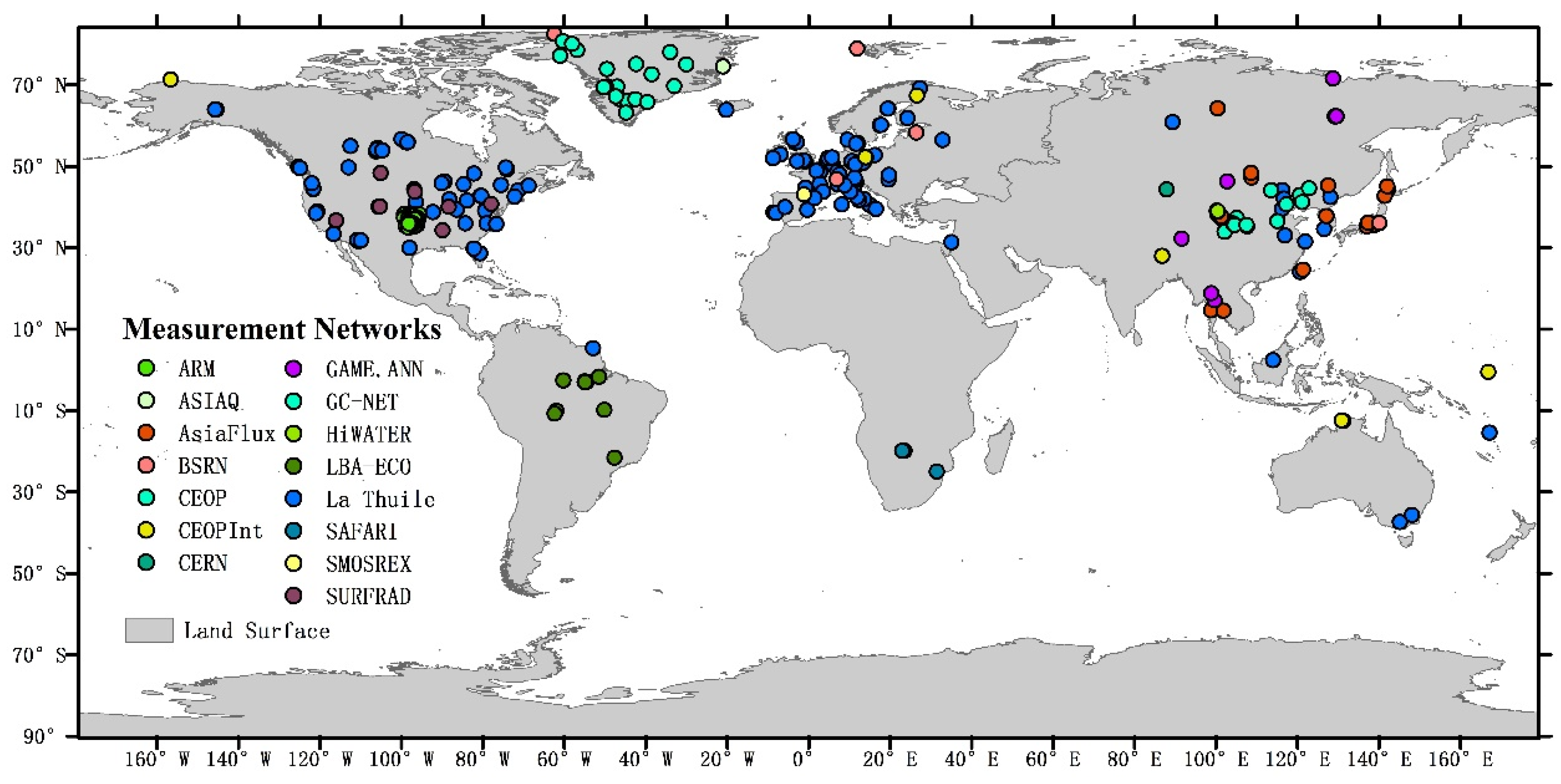
2.1.2. In Situ Observation Data

Observations taken from 15 measurement networks, shown in Figure 1, were collected, and the metadata for these measurement networks are given in Table 1 [26,27,28,29,30,31,32,33,34,35,36]. The sites are located around the Earth’s surface, representing different land cover types, such as forests (135 sites), scrublands (20 sites), grasslands (76 sites), bare lands (four sites), wetlands (18 sites), tundra (two sites), ice (23 sites), croplands (61 sites), and urban areas (one site). Some ground sites were eliminated from the monthly validation because their monthly in situ observations were less than 12.
Figure 1. Distribution of the 15 measurement networks.
Remotesensing 08 00090 g001
Table 1. Metadata for the 15 measurement networks.
Abbr.Full NameNum.URL
La ThuileLa Thuile dataset188[26]
CEOPCoordinated Enhanced Observation Network of China16\
CERNChinese Ecosystem Research Network1[27]
AsiaFluxAsiaFlux dataset19[28]
GAME.ANNGEWEX Asian Monsoon Experiment13\
SURFRADSurface Radiation Network7[29]
BSRNBaseline Surface Radiation Network5[30]
ARMAtmospheric Radiation Measurement29[31]
SMOSREXSurface Monitoring of Soil Reservoir Experiment1[32]
CEOPInt\7\
ASIAQAsiaq- Greenland Survey1[33]
GC-NETGreenland Climate Network21[34]
HiWATERHiWATER dataset20\
LBA-ECOThe Large-Scale Biosphere-Atmosphere Experiment in Ecology10[35]
SAFARIA Southern African Regional Science Initiative2[36]
Data from all those networks were checked site by site, and some extremely abnormal values were removed. Most networks had long time range observations, whereas CEOP and HiWATER in China had shorter time ranges and discontinuous observation data. All are trustworthy based on network control and continuous project support and have been utilized in many applications.

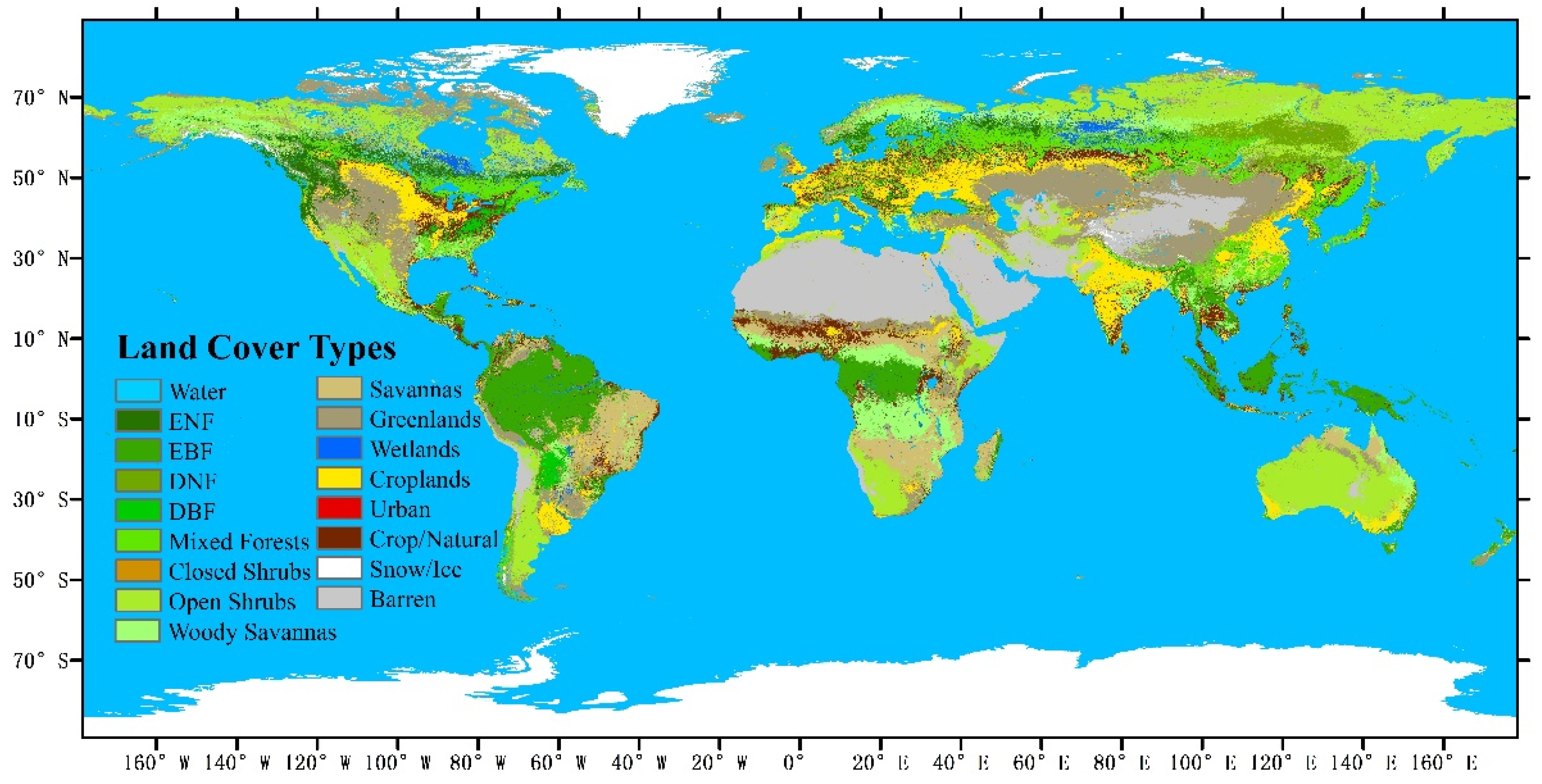
2.1.3. Land Cover Type Data

Given that the surface Rn is closely related to the land cover type, MCD12Q1 [37] land cover type data were used in this study, as shown in Figure 2 for reference.
Figure 2. Distribution of International Geosphere-Biosphere Program (IGBP) land cover types.
Remotesensing 08 00090 g002

2.1.4. Data for Attribution Analysis

As the sum of the four surface radiation components, Rn can be synthetically affected by many atmospheric and land surface conditions. Therefore, it is necessary to select multiple driving factors for further analysis in order to provide evidence to support the explanations for the variations in Rn. Normalized Difference Vegetation Index (NDVI), which characterizes the vegetation growth and coverage states, affected surface albedo directly [38]. Additionally, vegetation also influences surface temperature and diurnal temperature range, and further surface longwave radiation [39]. The snow cover affects surface albedo that regulates USW. Albedo largely determines surface shortwave net radiation. Solar radiation significantly affects the Tm that determines the ULW directly as a feedback according to Stefan-Boltzmann law. As for atmospheric factors, both precipitation (Pre) and cloud cover (CC) affect the DSW and DLW [40]. In addition, Pre greatly affects vegetation growth. So, all of the chosen factors are helpful to analyze the Rn variations. The characteristics of these data are listed in Table 2.
Table 2. Metadata for the Driving Factors.
Driving FactorsSourcesUnitsSpace ResolutionTime ResolutionTime Range
Precipitation (Pre)Climatic Research Unit (CRU) TS3.22 Precipitation [41]mm0.5°monthly1.2000–12.2013
Cloud Cover (CC)Climatic Research Unit (CRU) TS3.22 Cloud Cover [41]%0.5°monthly1.2000–12.2012
Temperature Range (TΔ)CRU TS3.22 Diurnal Temperature Range [41]°C0.5°monthly1.2000–12.2013
Surface Mean Temperature (Tm)CRU TS3.22 Mean Temperature [41]°C0.5°monthly1.2000–12.2013
NDVIGLASS products [42,43]\0.05°8 days1.2000–12.2013
Snow Cover (SC)MODIS/Terra [44]%0.05°monthly1.2000–12.2013
AlbedoGLASS products [42,45,46]\0.05°8 days1.2000–12.2013
CRU datasets are based on interpolated station observations. Harris et al. [47] found that each variable of the CRU datasets agree tightly with the other published datasets at regional and global scales, such as mean temperature data of the University of Delaware (UDEL), precipitation data of the Global Precipitation Climatology Centre (GPCC), DTR from Vose et al. [48]. The GLASS products, which are spatiotemporally continuous, have long temporal ranges and higher spatial resolutions than the similar satellite products. They are produced from multiple satellite data but mainly from MODIS data for the period of 2000–2013 [42].

2.2. Methodology

2.2.1. Validation

The three-hourly surface Rn values were calculated from the four radiation components using Equation (1). As the CERES data were released in GMT, while ground sites were in local time, the CERES sample data were converted into local time formats and averaged to the daily values for use in the for daily validations. The CERES monthly sample data were used for the monthly validations.
Due to the fact that different measurement networks have different temporal resolutions and units, the observations were handled as follows: for calculating daily in situ observations, measurement data must be recorded in every hour of one day; for obtaining the monthly in situ observations, at least six daily data should be recorded every 10 days in one month (the daily data should be recorded for more than 18 days in February). If the data did not meet these conditions, they would be eliminated before the validation. We unified the units of measurement to be in W·m−2 and calculated the average for the daily/monthly in situ observations. This method is trustworthy and controls the data quality strictly. Data recorded at sites that did not have at least 12 samples were also eliminated. In total, there were 340 sites used for the daily validations and 260 sites used for the monthly validations.
In order to express the land cover complexity in a better way, land cover data were re-sampled from 0.5 km to 0.05°. The normalized square deviation of the merging pixels was then taken to be the new pixel value. The new dataset was called the “land cover complexity”. This dataset was the base map on which the ground sites were displayed, and used as a reference for comparing the land surface complexity. In additionally, we also made a complexity data set with a 1° resolution, matching the CERES data. The code names for the International Geosphere-Biosphere Program (IGBP) land cover types are shown in Table 3.
Table 3. Code Names of IGBP Land Cover Types.
Code NamesLand Cover TypesCode NamesLand Cover Types
0Water9Savannas
1Evergreen Needle leaf Forest10Grasslands
2Evergreen Broadleaf Forest11Permanent Wetland
3Deciduous Needle leaf Forest12Croplands
4Deciduous Broadleaf Forest13Urban and Built-Up
5Mixed Forests14Cropland/Natural Vegetation
6Closed Shrublands15Snow and Ice
7Open Shrublands16Barren or Sparsely Vegetated
8Woody Savannas
The Mean Bias Error (MBE), Root-Mean-Square Error (RMSE), and coefficient of determination (R2) were selected to measure the validation results.

2.2.2. Spatiotemporal Analysis

The monthly CERES Rn data were chosen for the spatiotemporal analysis, but also aggregated to seasonal and annual scales. The driving factor datasets have different spatial and temporal resolutions, which are higher than those of the CERES. Before beginning the quantitative analysis, we re-sampled all of the datasets at a resolution of 1°, using the following principles. If all the merging pixels have no null values, average them directly. In the case where the number of null merging pixels is more than 60% of the total, this new pixel value is judged a null value. If the number of null pixels is less than 60%, take the average of the remaining non-null values as the new pixel value. All the datasets are re-sampled to obtain monthly mean values (the NDVI re-sampling is based on the maximum pixel value of each month). If the time range of the data recorded in a month is less than 20 days, the data in that month are excluded.
The effects of the driving factors on the Rn were analyzed using general linear models (GLMs) [49]. First, we obtained the correlation coefficient (R) between the driving factors and the Rn. Then, the driving factors entering the model were selected by a forward stepwise procedure by correlation order [50]. When adding a new independent variable or driving factor into the GLMs, the explained variance of the new model increases. We subtracted the previous explained variance to calculate the percentage sum of squares explained (%SS). However, the result cannot get rid of factors’ collinearity. The %SS of dependent driving factors may have a larger difference as the latter factor provides little information for the GLMs [51]. Considering the limitations of the %SS, the partial least squares (PLS) regression [52] was developed and combined with the variable importance in the projection (VIP) scores to be used in a further analysis. The aim of this further analysis was to characterize the relative importance of these driving factors, in terms of their influence on the Rn dynamics. All of the independent variables are projected into principal components, and the VIP score of independent variable j can be represented mathematically:
V I P j = k h = 1 m r 2 ( Y , c h ) w h j 2 h = 1 m r 2 ( Y , c h )
where k is the number of independent variable; ch is the one of m principal components; r(Y, ch) is the correlation index between ch and dependent variable Y; whj is the weight of independent variable j for ch. Thus, the PLS regression is the combination of multivariable linear regression modeling, correlation analysis, and principal components analysis, showing its strength when the independent variables are interrelated and when there are fewer data samples available [53].

3. Results Analysis and Discussion

3.1. Validation of the CERES Rn Product

3.1.1. Daily Scale

The daily CERES Rn samples, from March 2000 to July 2014, were compared with the observations taken from 340 sites. The resulting density of scatter diagram is shown in Figure 3.
Figure 3. Density of scatter plot of the CERES and in situ daily samples.
Remotesensing 08 00090 g003
Figure 3 indicates that the daily CERES Rn data show a strong consistency with the in situ observations. The MBE of the CERES data samples was 3.43 W·m−2, the RMSE was 33.56 W·m−2, and the R2 was 0.79. The MBE was positive, therefore showing that the CERES Rn data are slightly larger than the in situ observations.
The validation results of the CERES Rn, at each site, are shown in Figure 4. The grey scale represents the land cover complexity, to be used as a reference.
The MBE and RMSE values, at a number of sites in China, are much larger than most sites in Europe and America. This may be related to the measurement accuracy of different networks, as, for example, the La Thuile and the ARM networks have higher accuracy requirements. Compared with other networks, the CEOP, HiWATER, and CEOPInt, built in China, have poorer data continuity and a lower quantity of data. The CERES accuracy in Greenland appears to be lower. Inamdar et al., also found the CERES net shortwave radiation has large errors in the underlying surface snow [54]. The CERES Rn showed bad performance on a site in the central southern region of the United States. By checking the 0.05° land cover complexity results, we determined that this site is located on a more complicated underlying surface. Considering that the CERES Rn showed strong agreement with other sites in this region, the accuracy is still considered trustworthy.
Figure 4. Daily validation results of the CERES Rn data at individual sites (a) MBE; (b) RMSE; and (c) R2.
Remotesensing 08 00090 g004

3.1.2. Monthly Scale

The monthly CERES Rn samples were compared with the observations taken from 260 sites. The resulting density of scatter diagram is shown in Figure 5.
Figure 5. Density of scatter plot of the CERES and in situ monthly samples.
Remotesensing 08 00090 g005
At a monthly scale, the MBE was 3.40 W·m−2, the RMSE was 25.57 W·m−2, and the R2 was 0.84. This indicates that the CERES Rn data are slightly larger than the in situ observations, regardless of noise.
The validation results, at each ground site, are displayed in Figure 6.
Compared with the daily validation results, the performance of the monthly product is much better. It should be noted that there appears to be a poorer precision at a number of sites near the coast, and in Greenland. This reduction in precision may be caused by the large pixel areas with higher land cover complexity. Both daily validation and monthly validation showed lower accuracy of CERES Rn over Greenland.
The preprocessing of in situ data and CERES data was very strict, and the results are trustworthy. The validation results demonstrate that the CERES Rn product is, overall, highly accurate, although the accuracy is slightly lower for high latitudes.
Figure 6. Monthly validation results of the CERES Rn data at individual sites (a) MBE; (b) RMSE; and (c) R2.
Remotesensing 08 00090 g006aRemotesensing 08 00090 g006b

3.2. Spatiotemporal Analysis

3.2.1. Global Analysis of Rn

The monthly CERES Rn data, from 2001 to 2013, were used to detect the mean values of the Rn and annual trends in the Rn across the land surface, as showed in Figure 7. Data from years 2000 and 2014 covered less than one full year and were used only for the seasonal analysis.
There are entirely different distributions and trends of the Rn across the land surface over the past 13 years. It is evident that Rn, in some regions, has been increasing, such as in Greenland, the African tropical rainforest regions, the southeast of Brazil, the coast of Antarctica, and the west of Australia. Over the southwest of Greenland, Rn increased the fastest, at a rate of 4.21 W·m−2 per year. Conversely, there are some regions where Rn has decreased over time, such as in the southeast of Argentina, the African savannah, the southern Great Plains, and especially on the eastern side of the Andes Mountains, where Rn has decreased at a rate of 5.10 W·m−2 per year.
Figure 7. Mean values of the Rn from 2001 to 2013 (a); and annual trend of the Rn (b). The pixels in (b) marked with a dot indicate their statistical significance, with p-values < 0.05.
Remotesensing 08 00090 g007
In order to understand what caused these significant changes, we selected two geographical hotspot regions (the southern Great Plains and south-central Africa, where significant changes happened, the CERES Rn product and ancillary data for attribution analysis are relatively accurate), marked by the thick lines in Figure 7, for further analysis.

3.2.2. Southern Great Plains

The Great Plains is a well-known geographic area of the United States, and its southern chosen region covers parts of Colorado, Kansas, New Mexico, Oklahoma, and Texas [55]. This region is a major cotton and wheat production area of the U.S., and animal husbandry is another important industry [56]. The distribution of surface Rn influences its continental arid climate, which determines the agricultural yield and husbandry production in this region. Moreover, this region includes Tornado Alley [57]; the Rn variation affects the wind speed, which causes sand–dust disasters and tornadoes. The southern Great Plains is currently experiencing a remarkable decrease in Rn.
The temporal trend of the Rn over the Southern Great Plains was determined by a linear regression. The annual and seasonal trend plots were generated, and shown in Figure 8. The four seasons are conventionally defined as spring (March, April, and May), summer (June, July, and August), autumn (September, October, and November), and winter (December, January, and February).
Figure 8. Annual and seasonal trends of Rn over the southern Great Plains. The pixels marked with a dot indicate their statistical significance, with p-values < 0.05. Units: W·m−2 per year. (a) annual trend; (b) trend in spring; (c) trend in summer; (d) trend in autumn; and (e) trend in winter.
Remotesensing 08 00090 g008
The Rn decreased over the entire southern Great Plains by −0.33 W·m−2 per year. The fastest decrease occurred in summer, with a gradient of −0.58 W·m−2 per year, while the slowest decrease in spring was only −0.09 W·m−2 per year. Furthermore, the Rn decreased in the central region, and increased in the west edge. In the summer, the central part decreased sharply at a rate of −2.41 W·m−2 per year. However, also in the summer, the Rn in the northwest increased with a gradient of 1.62 W·m−2 per year. Rn in the east flat area did not show any significant trend.
In the significantly changing areas, the correlation analysis was carried out and %SS values were calculated between the CERES Rn and the driving factors, as shown in Table 4.
Table 4. Statistics for the correlation coefficient (R) and percentage sum of squares explained (%SS) between the Rn and the driving factors for the southern Great Plains. Numbers marked with a * indicates p-values < 0.10, and ** indicates p-values < 0.05, in which case the results are deemed to be significant. R stands for the correlation coefficient, Rn for the net radiation, Pre for precipitation, CC for cloud cover, TΔ for temperature range, Tm for surface temperature, and SC for snow cover.
AnnualSpringSummerAutumnWinter
R%SSR%SSR%SSR%SSR%SS
Rn and Pre0.47 *5−0.1620.26250.021−0.450
Rn and CC0.56 **16−0.0500.60 **360.1713−0.47 *4
Rn and TΔ−0.77 **12−0.030−0.53 **0−0.0900.290
Rn and Tm−0.150−0.040−0.3980.2520.71 **2
Rn and Albedo−0.270−0.1234−0.58 **4−0.3512−0.77 **8
Rn and NDVI0.71 **510.0630.60 **50.71 **500.668
Rn and SC−0.1180.132−0.131−0.343−0.78 **62
At an annual scale, NDVI explained 51% of the Rn variation, and CC explained 16%. In the spring, albedo explained 34% of the Rn variation. The lower %SS of the NDVI and SC may be caused by the co-linearity in the GLMs. In summer, CC and Pre played an important role, accounting for 61% of the Rn variation together. In autumn, NDVI explained 50% of the Rn variation. In winter, SC explained 62% of Rn variation.
However, due to the relevant dependency of certain variables within the GLMs (for example, albedo and SC in the winter), some factors cannot be used individually in an explanatory capacity. Additionally, the majority of correlation coefficients were not significant. Therefore, we conducted a further analysis utilizing the PLS regression to deal with the problems brought on by the interrelated nature of these driving factors. The VIP scores of these driving factors are shown in Figure 9.
Figure 9. Variable importance in the projection (VIP) scores of the driving factors in the southern Great Plains.
Remotesensing 08 00090 g009
Considering the %SS and VIP scores, it is clear that NDVI and TΔ were more dominating at an annual scale. Pre and CC effects also performed noticeably well. We think that the decreasing NDVI increased the albedo in the southern Great Plains, which affected the Rn in shortwave net radiation, and declining vegetation caused the larger TΔ and negative correlation with Rn, which affected the longwave net radiation. CC and precipitation affected the DSW and the decreasing precipitation or drought might be one of the reasons that influenced the NDVI. In the spring, precipitation, SC, and albedo were the key factors. SC changed the albedo and affected the USW so they were negatively correlated with Rn, and precipitation in the spring often was in the form of snow, further affecting the USW, especially of the western higher altitude areas.
In the summer, many factors, such as CC, TΔ, Tm, albedo, and NDVI, have large VIP scores. The CC, which reduces the DSW, showed positive correlation with Rn notably. We think that DSW was ample in the summer, as the NDVI decreased and albedo went up, more shortwave radiation was lost, longwave radiation played an important role in Rn variation. The Tm performance provided the proof to support this viewpoint, while CC might just decrease matched with Rn variation due to little rainfall, and fewer CC decreased the DLW especially in the night, and increased the TΔ combined with fewer NDVI due to the heat preservation [58].
In autumn, the key factors were the NDVI and albedo. SC also became an active factor. NDVI and SC both affected the Rn by changing the albedo, so land cover types played a more vital role and atmospheric factors had limited influence.
In the winter, the SC and NDVI had the highest VIP scores. It is clear that snowfall increased the albedo and NDVI was easily affected by the SC and vegetation growth periodicity in the winter, so these two factors both affected the albedo, thus changing the Rn.
Overall, we deduced that the NDVI was the main driving factor in the southern Great Plains, and precipitation played an indispensable role.

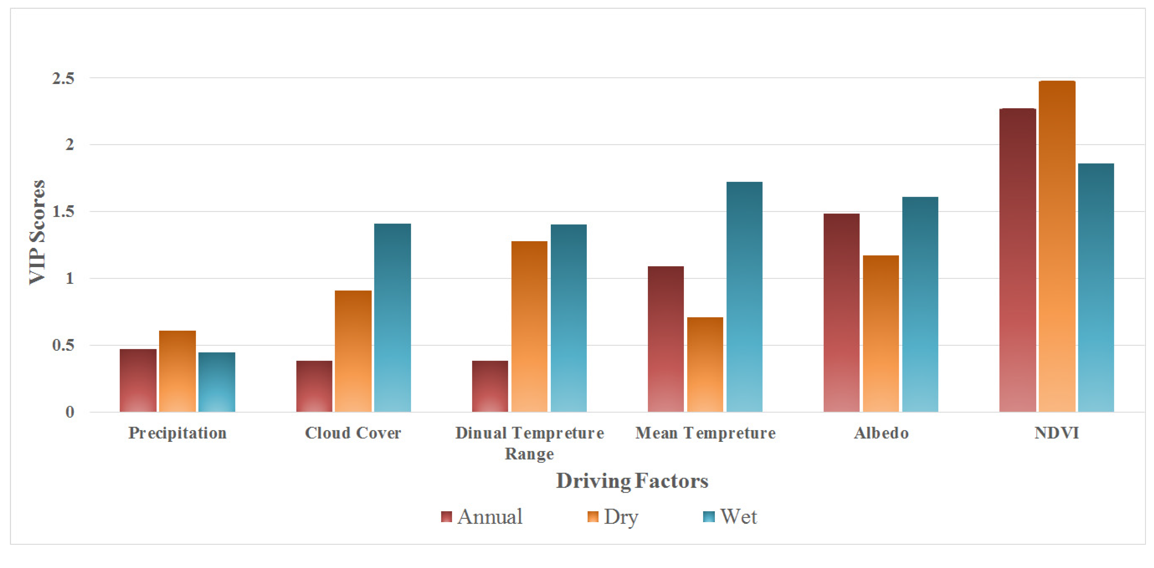
3.2.3. South-Central Africa

The second hot spot is situated in south-central Africa, including a majority of the Congo basin and part of the South African Veld. Abundant creatures and mineral resources exist in south-central Africa [59,60]. Countries located here are dominated by agriculture and mining industry. Therefore, understanding the Rn variation can help guide the population towards developing agriculture in a better way. Abundant flora and fauna exist in south-central Africa; the Rn variation could be an indicator of climate change that determines the habitat environment [61]. Therefore, research and protection of the biodiversity in this region is crucial. It is noteworthy that a clear decrease in Rn was observed. As this area has a tropical savanna climate, we performed the Rn variation analysis that is shown in Figure 10, separately, during the dry season (from May to October) and wet season (from the previous November to April).
Figure 10. Annual and seasonal trends of the Rn variation over south-central Africa. The pixels marked with a dot indicate their statistical significance, with p-values < 0.05. Units: W·m−2 per year. (a) annual trend; (b) trend in dry seasons; and (c) trend in wet seasons.
Remotesensing 08 00090 g010
In the annual analysis, the Rn decreased at a rate of −0.63 W·m−2 per year, overall. The dry season decreased at a slower rate of −0.39 W·m−2 per year, whereas the wet season decreased at a faster rate of −0.82 W·m−2 per year. With the exception of the western and eastern coasts, the Rn for the majority of south-central Africa was observed to decrease. The correlation analysis and %SS were calculated, and are shown in Table 5. South-central Africa had very little snow cover, and therefore the SC factor was excluded from the analysis.
Table 5. Statistics for the R and %SS between the Rn and the driving factors in south-central Africa. Numbers marked with a * indicates p-values < 0.10 and ** indicates p-values < 0.05, in which case the results are deemed to be significant.
AnnualDry SeasonWet Season
R%SSR%SSR%SS
Rn and Pre0.1520.112−0.123
Rn and CC−0.1000.240−0.391
Rn and TΔ0.060−0.3720.399
Rn and Tm0.3780.1520.48 *5
Rn and Albedo−0.52 *1−0.34100.446
Rn and NDVI0.80 **630.75 **560.51 *26
It is clear that the NDVI was the dominant driving factor. It had the largest explanatory power, accounting for more than 50% of the Rn variation for both the annual and dry season analyses. The albedo showed higher correlation with Rn but limited %SS. The results likely occurred because albedo does not provide more information than NDVI owing to the collinearity with NDVI. Tm showed a positive correlation with Rn; it is widely accepted that Tm determines the ULW but is affected by the shortwave radiation. We conclude that shortwave radiation was the major part of the surface radiation budget here in the wet season. Considering the limitation mentioned previously, the VIP scores of the driving factors in south-central Africa are shown in Figure 11.
Figure 11. Variable importance in the projection (VIP) scores of the driving factors in south-central Africa.
Remotesensing 08 00090 g011
The VIP scores corresponded very well with the %SS. No matter what period it is, the NDVI is the major driving factor, and we thought that the albedo, here, was also predominantly affected by this factor, as we infered from %SS. Additionally, the Tm had a significant impact during the wet season compared with the dry season. The Pre and CC had limited impact on the variation of the Rn during the annual analysis and dry season. CC in the wet season got higher VIP scores; we inferred that the increase of CC resisted more DSW, which controlled the surface radiation budget as we discussed. CC also influenced the TΔ and they got similar performance in all time, and precipitation had little variation in all time period so it had limited impact on Rn variation. It was hypothesized that the variation of Rn was perhaps caused by the degradation of forests and grassland due to drought in the dry season and human activities.
However, several uncertainties should be discussed. The accuracy of the atmospheric factors obtained from the CRU in Africa is not as high as the data in the southern Great Plains owing to the lower number of sites. Harris et al. [47] compared the CRU mean temperature data with data from UDEL in southern Africa and detected highly similar trends with a correlation coefficient of 0.91. Precipitation data were also compared with GPCC data with a correlation index of 0.89. Therefore, the CRU data are still trustworthy in this region. The reasons behind the high number of non-significant correlation coefficients were analyzed and were outlined here: (1) the R was calculated over areas with distinctly changing Rn, which includes different land cover types. Different underlying surfaces and elevation may lead to the different, or even contradictory, relationships between the Rn and the driving factors; (2) the time range of the CERES is short; and (3) the Rn can be influenced by many driving factors, and the Rn, itself, can influence the land surface or sky conditions though negative feedbacks.

4. Conclusions

There is a vast potential for developing remote sensing for use in determining the SRB, and the CERES product has become one of the most representative products. However, with a low number of in situ sites and poor distribution of CAVE sites, additional validation efforts are still required in order to determine the global accuracy of the CERES radiation products. This study validated the CERES Rn product close to the earth’s land surface at daily and monthly basis, and analyzed its spatiotemporal variation from 2001 to 2013. Two hot spot regions (the southern Great Plains and south-central Africa) were then selected for use in determining the driving factors. The conclusions of this study are summarized in the following points:
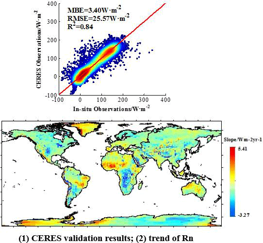
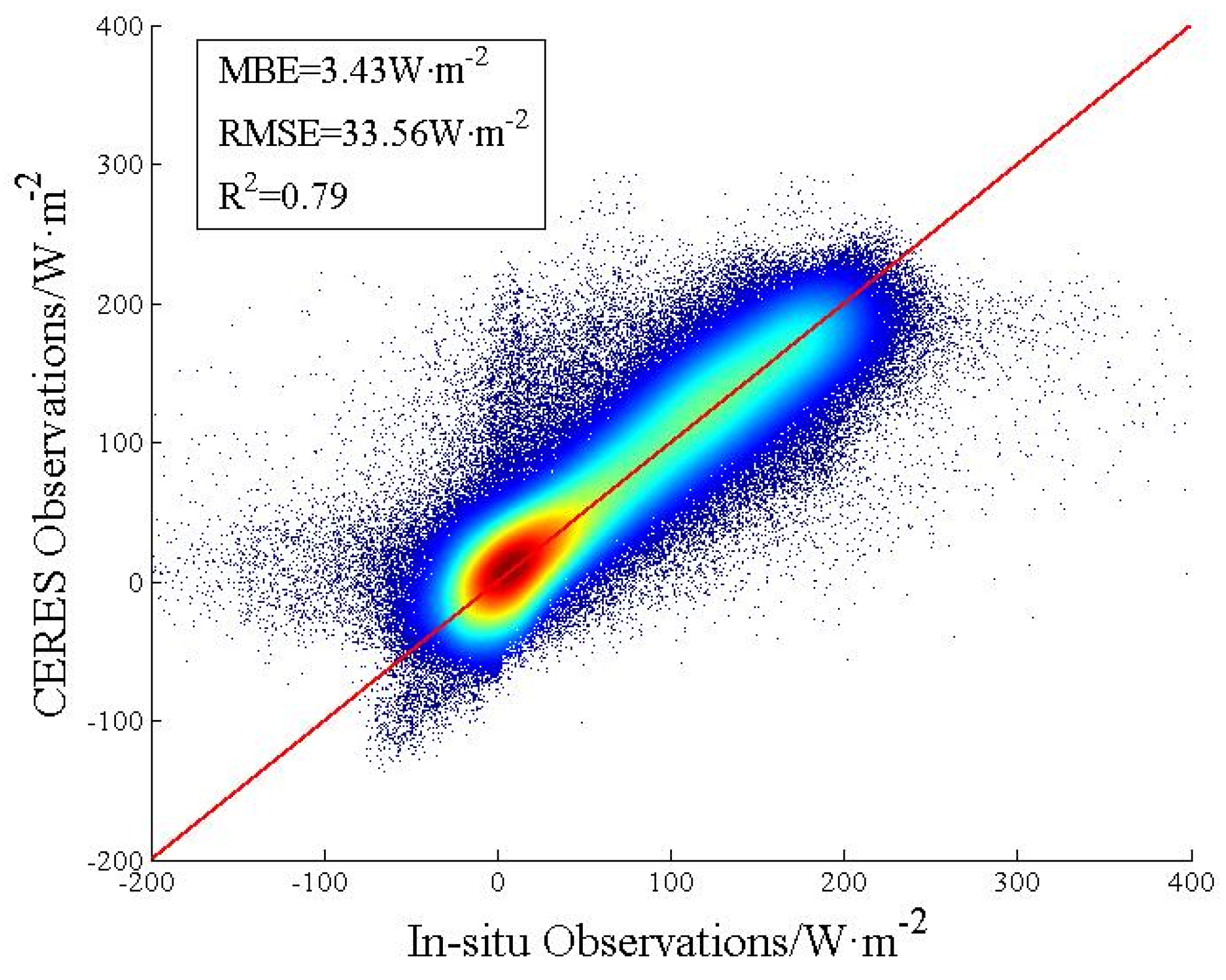
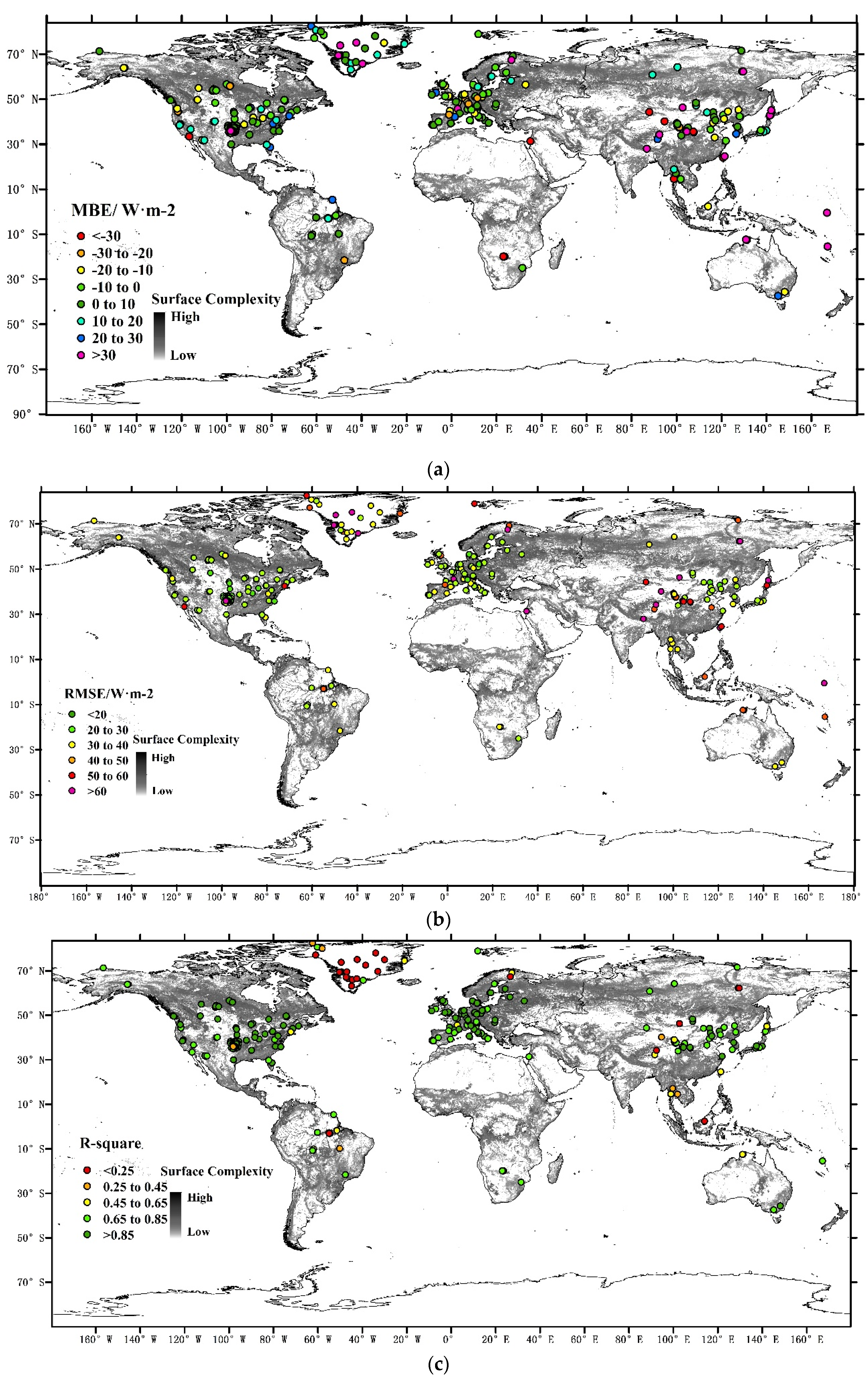
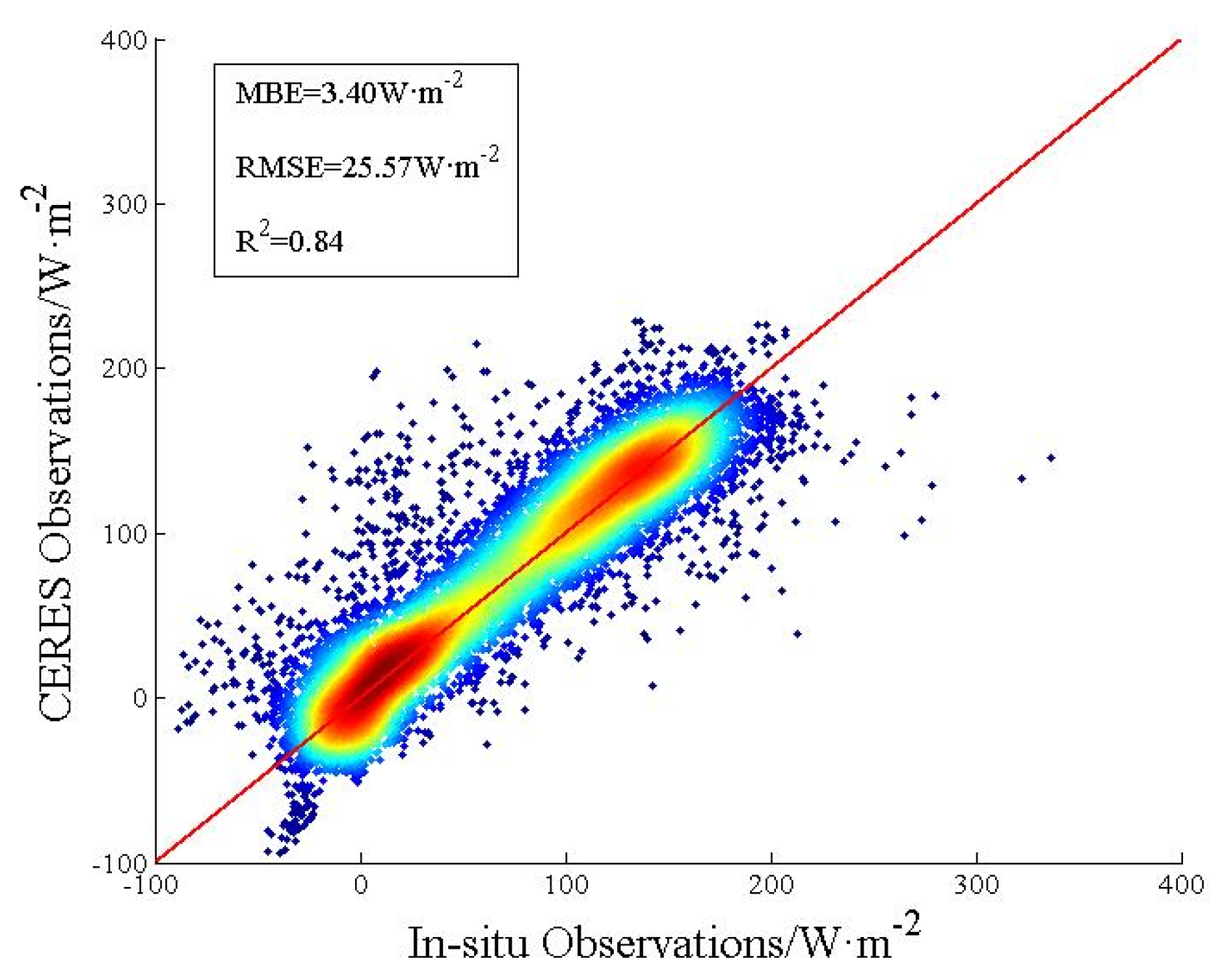
  • This paper validated the CERES_SYN1deg_Ed3A all-sky surface Rn at a daily and monthly basis, respectively. The daily validations had an MBE of 3.43 W·m−2, RMSE of 33.56 W·m−2, and R2 of 0.79. The monthly validations had an MBE of 3.40 W·m−2, RMSE of 25.57 W·m−2, and R2 of 0.84. Considering that the CERES_Ed2b was previously found to have a systematic bias of 14~21 W·m−2 [16], the integral accuracy of the CERES_SYN1deg_Ed3A is high enough for use in scientific research.
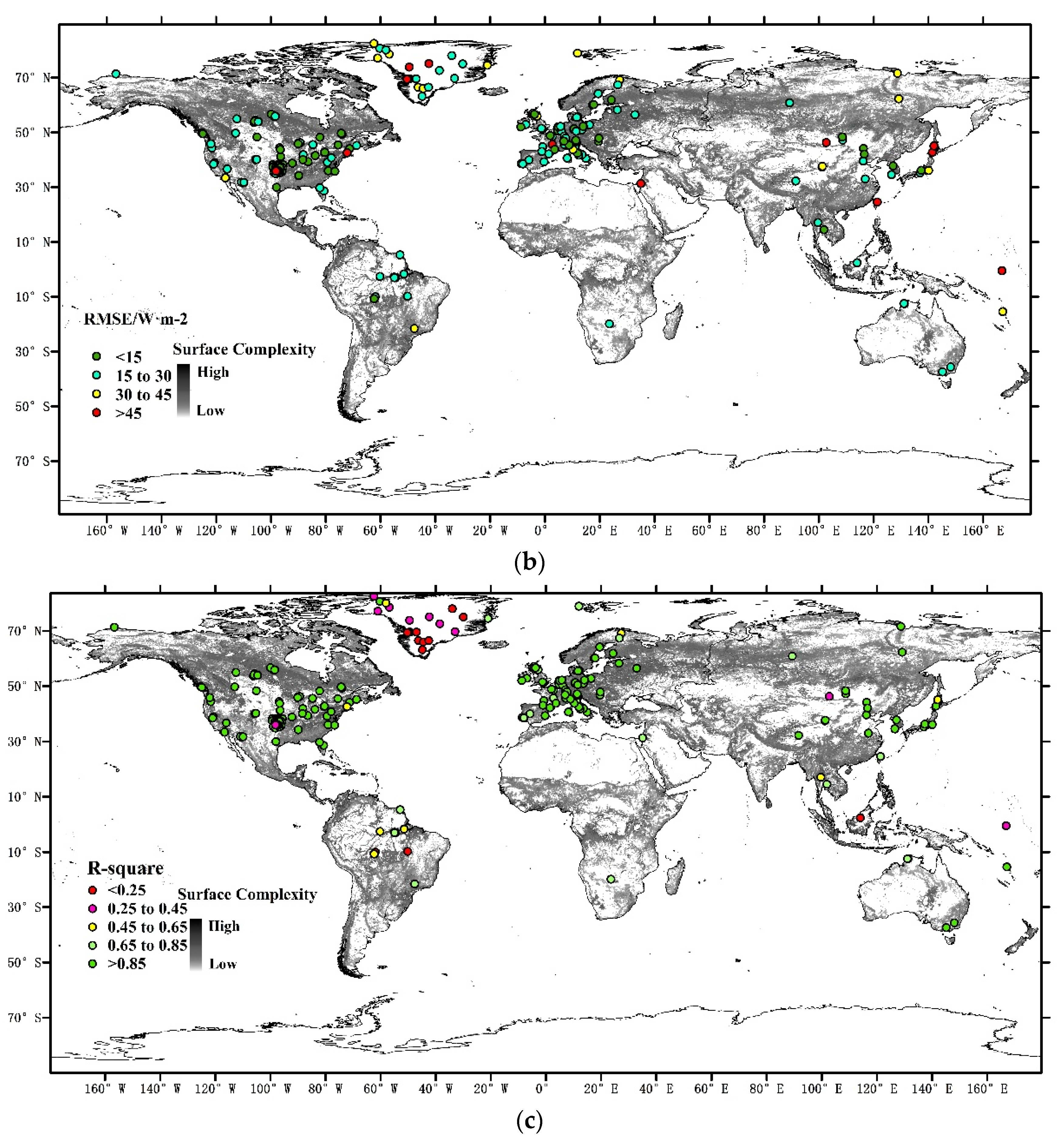
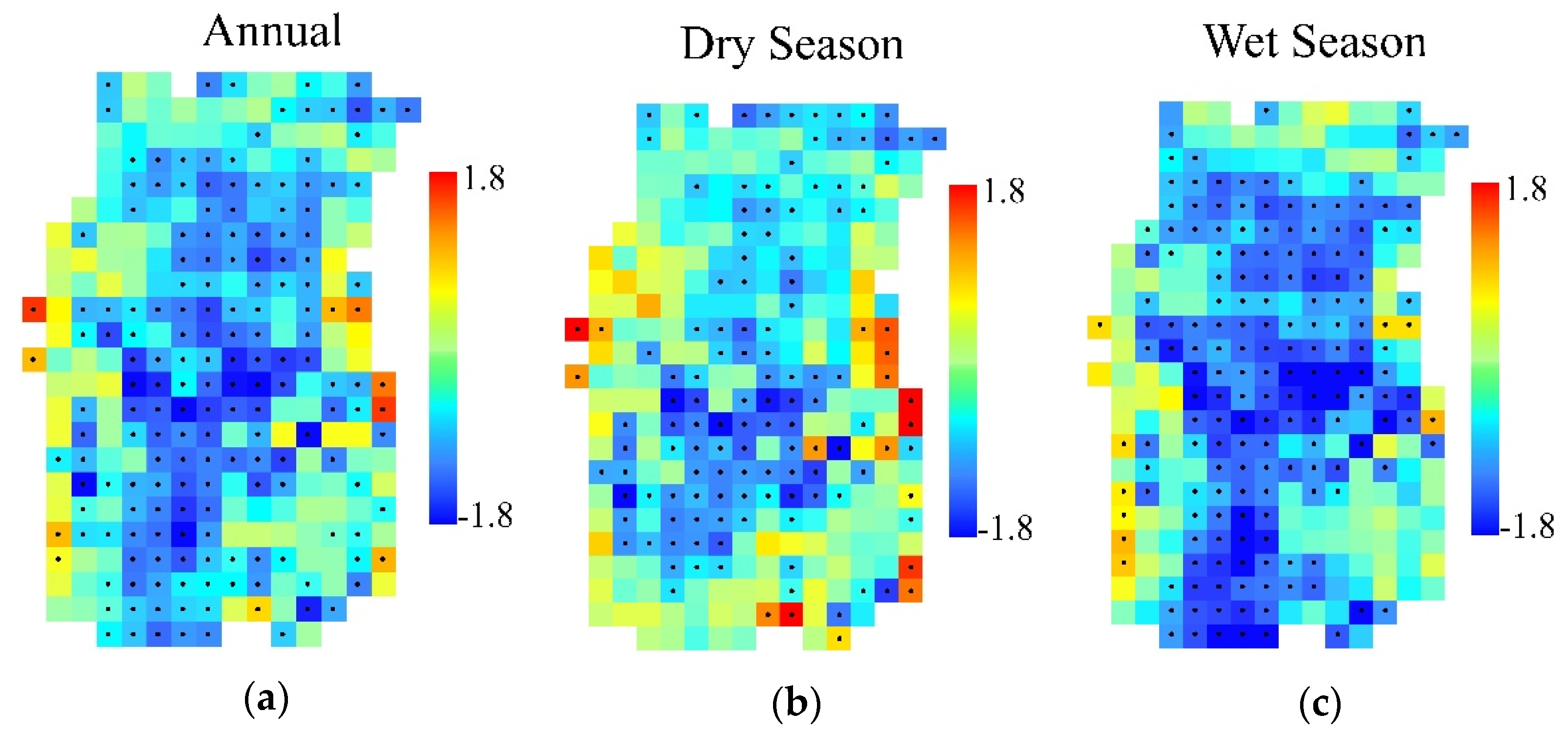
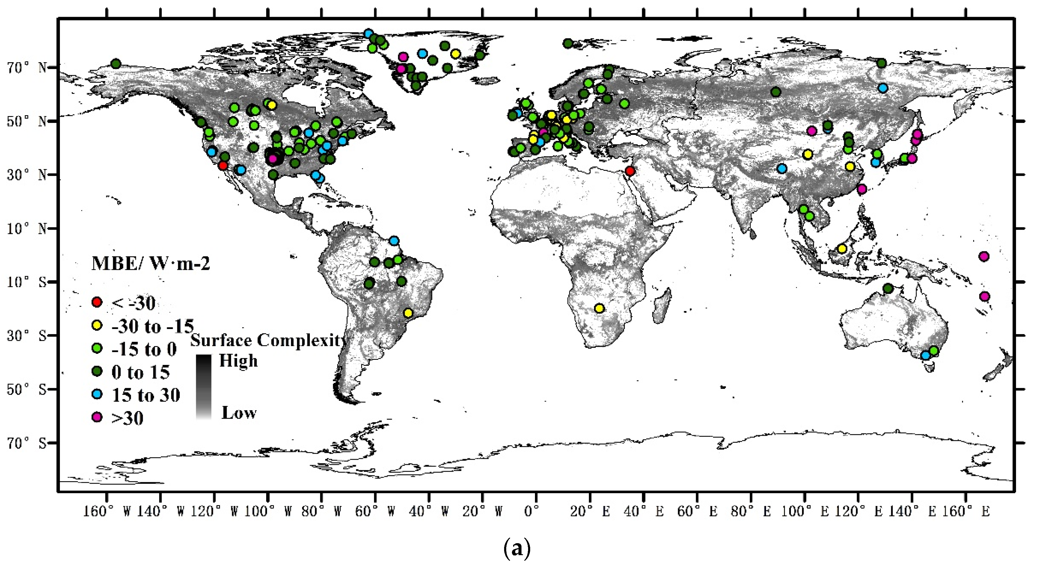
  • The accuracy distribution of the daily and monthly CERES Rn products were calculated. It was found that areas in the middle and low latitudes had a higher accuracy, and that the R2 was lower for areas in the high latitudes, such as Greenland. This may be caused by the lower accuracy of CERES inversion over the snow surface. The uncertainty near the coast was caused by the coarse resolution of the CERES products matching with in situ observations.
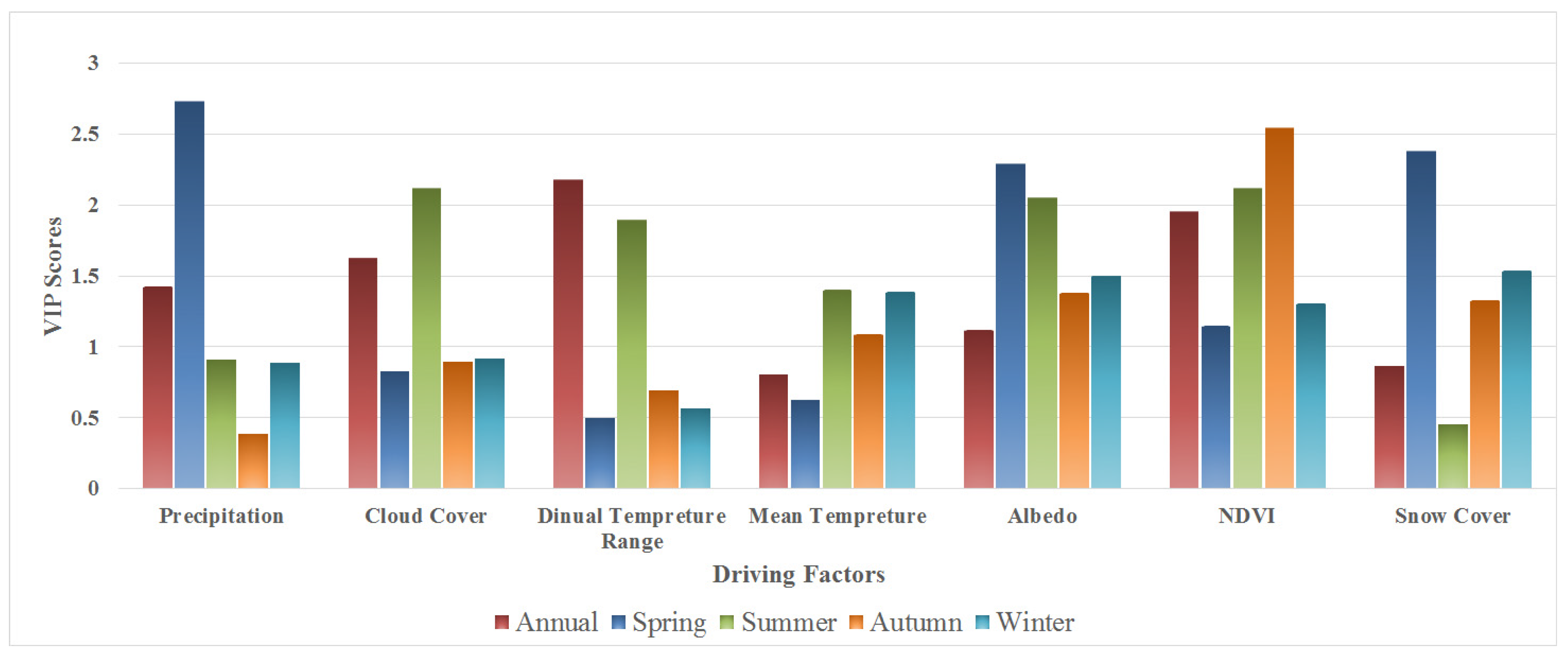
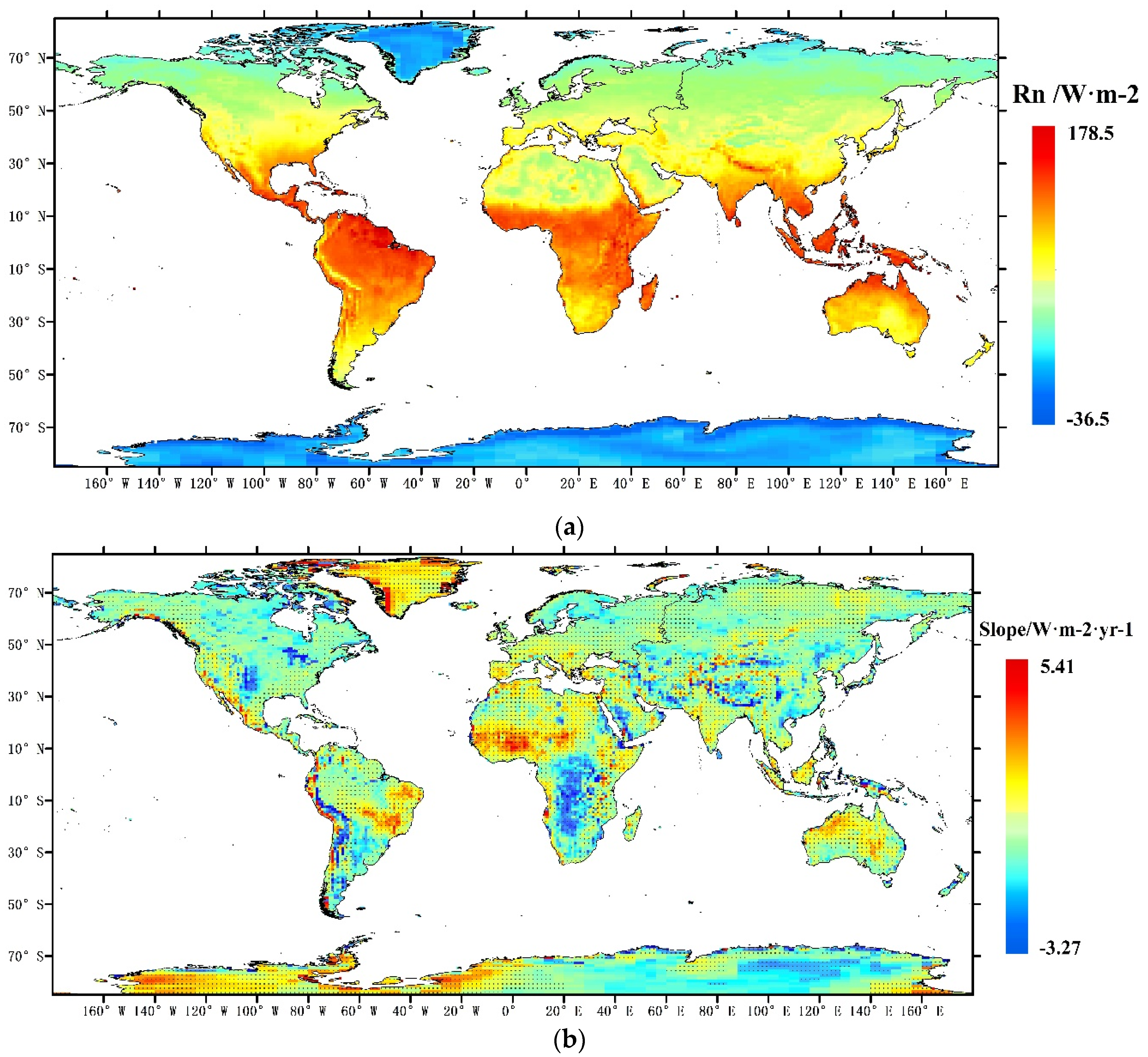
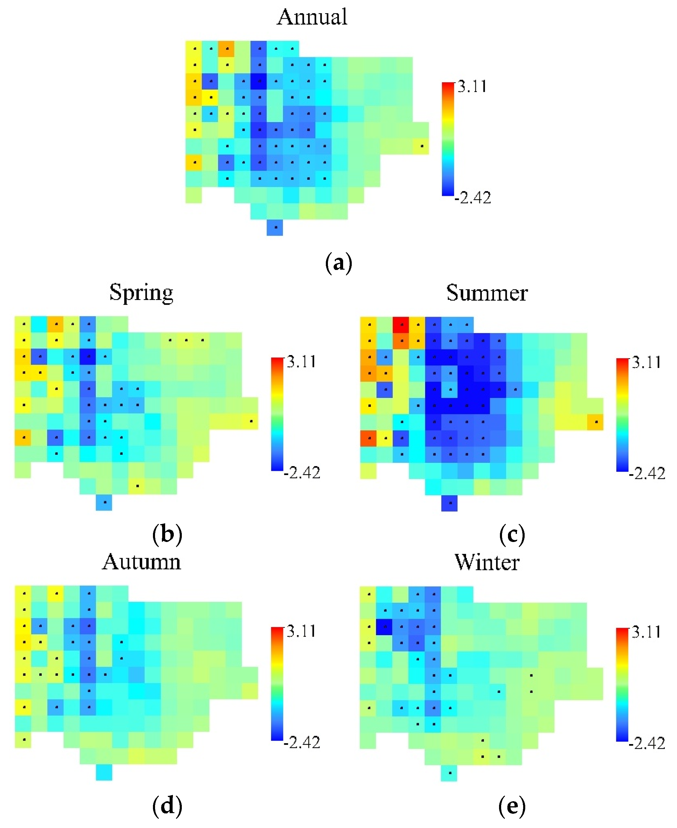
  • This study analyzed the spatiotemporal variation of the monthly CERES Rn, from 2001 to 2013, and found that different regions exhibited vastly differing rates of change. In terms of the hot spot analysis, the Rn decreased slightly over the entire southern Great Plains, with a gradient of −0.33 W·m−2 per year. As for the attribution analysis, percentage sum of squares explained and VIP scores were calculated. From the annual and seasonal analysis, we concluded that NDVI, which represents the surface vegetation condition, was the major driving factor of the Rn variation over the southern Great Plains and that precipitation played an indispensable role. We determined that little precipitation was one of reasons for the deterioration of the vegetation. Moreover, barren soil increased the TΔ and added more ULW. In the winter, SC was the main factor of Rn variation because it easily changed the albedo and controlled shortwave radiation. The Rn over south-central Africa decreased at a rate of −0.63 W·m−2 per year, with NDVI as the main driving factor. Regardless of the analysis period, NDVI was always the leading factor, as evidenced by the high VIP scores and %SS. Different from the case of the Great Plains, precipitation showed little correlation with Rn variation. This may be attributed to the little variation of precipitation, particularly during the wet season.
To identify the contributing factors that caused the changes in Rn in the two hotspots regions, CRU data were used. Although CRU data is based on interpolated ground stations, the data can be considered as, overall, reliable for our analysis in the hotspot regions.

Acknowledgments

This study was funded by the National High-Technology Research and Development Program of China under Grant 2013AA122800, the Natural Science Foundation of China (No. 41401381 and No. 41101310), the Special Foundation for Young Scientists of State Laboratory of Remote Sensing Science (grant 15RC-12), and the Fundamental Research Funds for the Central Universities under Grant 2013NT28. This work used the eddy covariance data acquired by the FLUXNET community and, in particular, by the following networks: AmeriFlux (U.S. Department of Energy, Biological and Environmental Research, Terrestrial Carbon Program (DE-FG02-04ER63917)), AfriFlux, AsiaFlux, CarboAfrica, CarboEuropeIP, CarboItaly, CarboMont, ChinaFlux, Fluxnet-Canada (supported by CFCAS, NSERC, BIOCAP, Environment Canada, and NRCan), GreenGrass, KoFlux, LBA, NECC, OzFlux, TCOS-Siberia, and USCCC. We acknowledge the financial support for the eddy covariance data harmonization provided by CarboEuropeIP, FAO-GTOS-TCO, Ileaps, Max Planck Institute for Biogeochemistry, National Science Foundation, University of Tuscia, Université Laval, Environment Canada, and the U.S. Department of Energy. Additionally, we acknowledge the dataset development and technical support provided by Berkeley Water Center, Lawrence Berkeley National Laboratory, Microsoft Research eScience, Oak Ridge National Laboratory, University of California—Berkeley, and the University of Virginia. We would also like to thank Yan Li and Ran Li from the Xinjiang Institute of Ecology and Geography, CAS, and Jean Christophe Calvet from CNRM-GAME for sharing their data.

Author Contributions

Bo Jiang and Shunlin Liang designed the experiment, Xiaotong Zhang collected the required data, Aolin Jia performed the experiment, Aolin Jia, Bo Jiang and Shunlin Liang conducted the analysis of the results, and all of the aforementioned contributed towards writing the manuscript.

Conflicts of Interest

The authors declare no conflict of interest.

References

  1. Liang, S. Quantitative Remote Sensing of Land Surfaces; John Wiley & Sons: Hoboken, NJ, USA, 2005; Volume 30. [Google Scholar]
  2. Wild, M.; Folini, D.; Schär, C.; Loeb, N.; Dutton, E.G.; König-Langlo, G. The global energy balance from a surface perspective. Clim. Dyn. 2013, 40, 3107–3134. [Google Scholar] [CrossRef]
  3. Liang, S.; Wang, K.; Zhang, X.; Wild, M. Review on estimation of land surface radiation and energy budgets from ground measurement, remote sensing and model simulations. IEEE J. Sel. Top. Appl. Earth Obs. Remote Sens. 2010, 3, 225–240. [Google Scholar] [CrossRef]
  4. Gui, S. Satellite Remote Sensing of Surface Net Radiation Doctor; Wuhan University: Wuhan, China, 2010. [Google Scholar]
  5. Jiang, B.; Zhang, Y.; Liang, S.; Wohlfahrt, G.; Arain, A.; Cescatti, A.; Georgiadis, T.; Jia, K.; Kiely, G.; Lund, M. Empirical estimation of daytime net radiation from shortwave radiation and ancillary information. Agric. For. Meteorol. 2015, 211, 23–36. [Google Scholar] [CrossRef]
  6. Jiang, B.; Zhang, Y.; Liang, S.; Zhang, X.; Xiao, Z. Surface Daytime Net Radiation Estimation Using Artificial Neural Networks. Remote Sens. 2014, 6, 11031–11050. [Google Scholar] [CrossRef]
  7. Wielicki, B.A.; Barkstrom, B.R.; Harrison, E.F.; Lee, R.B.; Louis Smith, G.; Cooper, J.E. Clouds and the Earth’s Radiant Energy System (CERES): An earth observing system experiment. Bull. Am. Meteorol. Soc. 1996, 77, 853–868. [Google Scholar] [CrossRef]
  8. Charlock, T.P.; Alberta, T.L. The CERES/ARM/GEWEX Experiment (CAGEX) for the retrieval of radiative fluxes with satellite data. Bull. Am. Meteorol. Soc. 1996, 77, 2673–2683. [Google Scholar] [CrossRef]
  9. Fu, Q.; Liou, K. Parameterization of the radiative properties of cirrus clouds. J. Atmos. Sci. 1993, 50, 2008–2025. [Google Scholar] [CrossRef]
  10. Rutan, D.A.; Charlock, T.P.; Rose, F.G.; Smith, N.M. CERES/ARM Validation Experiment. In Proceedings of the 11th Conference on Satellite Meteorology and Oceanography, Madison, WI, USA, 15–18 October 2001; pp. 606–609.
  11. Rutan, D.; Rose, F.; Smith, N.; Charlock, T. CERES/ARM Validation Experiment. In Proceedings of the 11th ARM Science Team Meeting, Atlanta, GA, USA, 19–23 March 2001; pp. 1–4.
  12. Rutan, D.A.; Charlock, T. Validation of CERES/SARB data product using ARM surface flux observations. In Proceedings of the 14th ARM Science Team Meeting Proceedings, Albuquerque, NM, USA, 22–26 March 2004.
  13. Gui, S.; Liang, S.; Li, L. In Validation of surface radiation data provided by the CERES over the Tibetan Plateau. In Proceedings of the 2009 17th International Conference on Geoinformatics, Fairfax, VA, USA, 12–14 August 2009; pp. 1–6.
  14. Wang, L.; Lü, D.; He, Q. The impact of surface properties on downward surface shortwave radiation over the Tibetan Plateau. Adv. Atmos. Sci. 2015, 32, 759–771. [Google Scholar] [CrossRef]
  15. Pan, X.; Liu, Y.; Fan, X. Comparative Assessment of Satellite-Retrieved Surface Net Radiation: An Examination on CERES and SRB Datasets in China. Remote Sens. 2015, 7, 4899–4918. [Google Scholar] [CrossRef]
  16. Kratz, D.P.; Gupta, S.K.; Wilber, A.C.; Sothcott, V.E. Validation of the CERES Edition 2B surface-only flux algorithms. J. Appl. Meteorol. Climatol. 2010, 49, 164–180. [Google Scholar] [CrossRef]
  17. Charlock, T.; Rose, F.G.; Rutan, D.A.; Jin, Z.; Su, W.; Rutledge, K.; Smith, W. Retrieval and Validation of Radiative Fluxes at the Ocean Surface with CIRES; World Meteorological Organization: Geneva, Switzerland, 2001; pp. 228–231. [Google Scholar]
  18. Charlock, T.; Rose, F.; Jin, Z.; Smith, W.; Rutledge, K.; Rutan, D. Validation of the CERES Surface and Atmospheric Radiation Budget Using the CLAMS Aircraft Campaign and COVE Ocean Platform; AGU Spring Meeting: Washington, DC, USA, 2002; p. 11. [Google Scholar]
  19. Wild, M.; Folini, D.; Hakuba, M.Z.; Schär, C.; Seneviratne, S.I.; Kato, S.; Rutan, D.; Ammann, C.; Wood, E.F.; König-Langlo, G. The energy balance over land and oceans: An assessment based on direct observations and CMIP5 climate models. Clim. Dyn. 2014, 44, 3393–3429. [Google Scholar] [CrossRef]
  20. Jiménez-Muñoz, J.C.; Sobrino, J.A.; Mattar, C. Recent trends in solar exergy and net radiation at global scale. Ecol. Model. 2012, 228, 59–65. [Google Scholar] [CrossRef]
  21. Gao, Y.; Honglin, H.E.; Zhang, L.; Qianqian, L.U.; Guirui, Y.U.; Zhang, Z. Spatio-temporal Variation Characteristics of Surface Net Radiation in China over the Past 50 Years. J. Geoinf. Sci. 2013, 15, 1–10. [Google Scholar] [CrossRef]
  22. Shi, Q.; Liang, S. Characterizing the surface radiation budget over the Tibetan Plateau with ground-measured, reanalysis, and remote sensing data sets: 2. Spatiotemporal analysis. J. Geophys. Res. Atmos. 2013, 118, 8921–8934. [Google Scholar] [CrossRef]
  23. Smith, G.; Priestley, K.; Loeb, N.; Wielicki, B.; Charlock, T.; Minnis, P.; Doelling, D.; Rutan, D. Clouds and Earth Radiant Energy System (CERES), a review: Past, present and future. Adv. Space Res. 2011, 48, 254–263. [Google Scholar] [CrossRef]
  24. Young, D.; Minnis, P.; Doelling, D.; Gibson, G.; Wong, T. Temporal interpolation methods for the Clouds and the Earth’s Radiant Energy System (CERES) experiment. J. Appl. Meteorol. 1998, 37, 572–590. [Google Scholar] [CrossRef]
  25. CERES Official Website. Available online: http://ceres.larc.nasa.gov/ (accessed on 15 March 2015).
  26. Fluxnet. Available online: http://www.fluxdata.org/ (accessed on 18 May 2014).
  27. CERN. Available online: http://www.cerndata.ac.cn/ (accessed on 21 May 2014).
  28. AsiaFlux. Available online: http://www.asiaflux.net/ (accessed on 22 April 2014).
  29. ESRL Global Mnotoring Division-Global Radiation Group. Available online: http://www.esrl.noaa.gov/gmd/grad/surfrad/ (accessed on 5 June 2014).
  30. BSRN-World Radiation Monitoring Center Baseline Surface Radiation Network. Available online: http://www.bsrn.awi.de/ (accessed on 11 April 2014).
  31. U.S. Department of Energy. ARM-Data. Available online: http://www.archive.arm.gov/ (accessed on 25 March 2014).
  32. Centre d’Etudes Spatiales de la BIOsphère. Available online: http://www.cesbio.ups-tlse.fr/ (accessed on 3 May 2014).
  33. Asiaq-Greenland Survey. Available online: http://www.archive.arm.gov/ (accessed on 16 April 2014).
  34. Greenland Climate Network (GC-Net). Available online: http://cires.colorado.edu/science/groups/steffen/gcnet/ (accessed on 27 March 2014).
  35. LBA-ECO. Available online: http://www.lbaeco.org/ (accessed on 14 March 2014).
  36. SAFARI. Available online: http://daac.ornl.gov/S2K/safari.shtml (accessed on 12 June 2014).
  37. Broxton, P.D.; Zeng, X.; Sulla-Menashe, D.; Troch, P.A. A global land cover climatology using MODIS data. J. Appl. Meteorol. Climatol. 2014, 53, 1593–1605. [Google Scholar] [CrossRef]
  38. Pettorelli, N.; Vik, J.O.; Mysterud, A.; Gaillard, J.-M.; Tucker, C.J.; Stenseth, N.C. Using the satellite-derived NDVI to assess ecological responses to environmental change. Trends Ecol. Evol. 2005, 20, 503–510. [Google Scholar] [CrossRef] [PubMed]
  39. Van de Griend, A.; Owe, M. On the relationship between thermal emissivity and the normalized difference vegetation index for natural surfaces. Int. J. Remote Sens. 1993, 14, 1119–1131. [Google Scholar] [CrossRef]
  40. Brutsaert, W. On a derivable formula for long-wave radiation from clear skies. Water Resour. Res. 1975, 11, 742–744. [Google Scholar] [CrossRef]
  41. Jones, P.D.; Harris, I. Climatic Research Unit (CRU) Time-Series Datasets of Variations in Climate with Variations in Other Phenomena; Centre for Environment Data: Didcot, UK, 2008. [Google Scholar]
  42. Zhao, X.; Liang, S.; Liu, S.; Yuan, W.; Xiao, Z.; Liu, Q.; Cheng, J.; Zhang, X.; Tang, H.; Zhang, X. The Global Land Surface Satellite (GLASS) remote sensing data processing system and products. Remote Sens. 2013, 5, 2436–2450. [Google Scholar] [CrossRef]
  43. Liang, S.; Zhao, X.; Liu, S.; Yuan, W.; Cheng, X.; Xiao, Z.; Zhang, X.; Liu, Q.; Cheng, J.; Tang, H. A long-term Global LAnd Surface Satellite (GLASS) data-set for environmental studies. Int. J. Digit. Earth 2013, 6, 5–33. [Google Scholar] [CrossRef]
  44. Hall, D.; Salomonson, V.; Riggs, G. MODIS/Terra Snow Cover Monthly L3 Global 0.05deg CMG; National Snow and Ice Data Center: Boulder, CO, USA, 2006. [Google Scholar]
  45. Liu, Q.; Wang, L.; Qu, Y.; Liu, N.; Liu, S.; Tang, H.; Liang, S. Preliminary evaluation of the long-term GLASS albedo product. Int. J. Digit. Earth 2013, 6, 69–95. [Google Scholar] [CrossRef]
  46. Liu, N.; Liu, Q.; Wang, L.; Wen, J. A temporal filtering algorithm to reconstruct daily albedo series based on glass albedo product. In Proceedings of the IEEE International Geoscience and Remote Sensing Symposium (IGARSS), Vancouver, BC, Canada, 24–29 July 2011; pp. 4277–4280.
  47. Harris, I.; Jones, P.; Osborn, T.; Lister, D. Updated high-resolution grids of monthly climatic observations—The CRU TS3. 10 Dataset. Int.J. Climatol. 2014, 34, 623–642. [Google Scholar] [CrossRef] [Green Version]
  48. Vose, R.S.; Easterling, D.R.; Gleason, B. Maximum and minimum temperature trends for the globe: An update through 2004. Geophys. Res. Lett. 2005, 32. [Google Scholar] [CrossRef]
  49. Wang, X.; Fang, J.; Sanders, N.J.; White, P.S.; Tang, Z. Relative importance of climate vs local factors in shaping the regional patterns of forest plant richness across northeast China. Ecography 2009, 32, 133–142. [Google Scholar] [CrossRef]
  50. Austin, M.; Pausas, J.G.; Nicholls, A. Patterns of tree species richness in relation to environment in southeastern New South Wales, Australia. Aust. J. Ecol. 1996, 21, 154–164. [Google Scholar] [CrossRef]
  51. Zhang, Y.; Liang, S. Changes in forest biomass and linkage to climate and forest disturbances over Northeastern China. Glob. Chang. Biol. 2014, 20, 2596–2606. [Google Scholar] [CrossRef] [PubMed]
  52. Næsset, E.; Bollandsås, O.M.; Gobakken, T. Comparing regression methods in estimation of biophysical properties of forest stands from two different inventories using laser scanner data. Remote Sens. Environ. 2005, 94, 541–553. [Google Scholar] [CrossRef]
  53. Wold, S.; Sjöström, M.; Eriksson, L. PLS-regression: A basic tool of chemometrics. Chemom. Intell. Lab. Syst. 2001, 58, 109–130. [Google Scholar] [CrossRef]
  54. Inamdar, A.K.; Guillevic, P.C. Net Surface Shortwave Radiation from GOES Imagery—Product Evaluation Using Ground-Based Measurements from SURFRAD. Remote Sens. 2015, 7, 10788–10814. [Google Scholar] [CrossRef]
  55. Rossum, S.; Lavin, S. Where are the Great Plains? A cartographic analysis. Prof. Geogr. 2000, 52, 543–552. [Google Scholar] [CrossRef]
  56. Browne, R.B. Encyclopedia of the Great Plains. J. Am. Cult. 2005, 28. [Google Scholar] [CrossRef]
  57. Perkins, S. Tornado alley, USA: New map defines nation’s twister risk. Sci. News 2002, 161, 296–298. [Google Scholar] [CrossRef]
  58. Dai, A.; Trenberth, K.E.; Karl, T.R. Effects of clouds, soil moisture, precipitation, and water vapor on diurnal temperature range. J. Clim. 1999, 12, 2451–2473. [Google Scholar] [CrossRef]
  59. Cowling, R.M.; Richardson, D.M.; Pierce, S.M. Vegetation of Southern Africa; Cambridge University Press: Cambridge, UK, 2004. [Google Scholar]
  60. Hamann, R.; Kapelus, P. Corporate social responsibility in mining in Southern Africa: Fair accountability or just greenwash? Development 2004, 47, 85–92. [Google Scholar] [CrossRef]
  61. Tyson, P.D.; Preston-Whyte, R.A. Weather and Climate of Southern Africa; Oxford University Press: Oxford, UK, 2000. [Google Scholar]

