Dynamic Mapping of Evapotranspiration Using an Energy Balance-Based Model over an Andean Páramo Catchment of Southern Ecuador

Abstract

Understanding of evapotranspiration (ET) processes over Andean mountain environments is crucial, particularly due to the importance of these regions to deliver water-related ecosystem services. In this context, the detection of spatio-temporal changes in ET remains poorly investigated for specific Andean ecosystems, like the páramo. To overcome this lack of knowledge, we implemented the energy-balance model METRIC with Landsat 7 ETM+ and MODIS-Terra imagery for a páramo catchment. The implementation contemplated adjustments for complex terrain in order to obtain daily, monthly and annual ET maps (between 2013 and 2014). In addition, we compared our results to the global ET product MOD16. Finally, a rigorous validation of the outputs was conducted with residual ET from the water balance. ET retrievals from METRIC (Landsat-based) showed good agreement with the validation-related ET at monthly and annual steps (mean bias error <8 mm·month⁻¹ and annual deviation <17%). However, METRIC (MODIS-based) outputs and the MOD16 product were revealed to be unsuitable for our study due to the low spatial resolution. At last, the plausibility of METRIC to obtain spatial ET retrievals using higher resolution satellite data is demonstrated, which constitutes the first contribution to the understanding of spatially-explicit ET over an alpine catchment in the neo-tropical Andes.

1. Introduction

The importance to investigate the hydrological responses of tropical mountains to climate change scenarios [1,2,3,4,5] and also to the influence of land cover changes [6,7,8,9] lies in the imperative conservation of water resources and the tropical mountain environment. One of the main hydrological response variables is evapotranspiration (ET). This water depletion key indicator plays a fundamental and still poorly understood role in water regulation processes, particularly in highland areas. Therefore, accurate area-wide estimates of ET over mountain environments is crucial for the sustainable management of water resources and the conservation of pristine ecosystems like the páramo, a high and humid neo-tropical alpine grasslands in the Andean cordillera of South America [10].

Only a few studies of reference ET at the point scale have been conducted in this ecosystem [11,12], considering that ET is hardly assessable in space with field measurements. To overcome this problem, remote sensing-based models for spatial ET estimation are under evolution with important improvements in accuracy levels reported during the last decade [13,14,15,16,17,18,19,20,21,22,23] using diverse approaches. The METRIC approach (Mapping EvapoTranspiration at high Resolution with Internalized Calibration) developed by Allen et al. [24] is a state-of-the-art model for mapping actual ET using satellite imagery with the thermal infrared band. METRIC and its predecessor SEBAL [25] are similar to other energy balance-based models, such as the Two-Source Energy Balance (TSEB) model [26], Surface Energy Balance System (SEBS) model [27], Simple Remote Sensing EvapoTranspiration (sim-ReSET) model [28], Two-Source Model (TSM) [29] and the Atmosphere-Land Exchange Inverse (ALEXI) model [30]. These approaches can deliver representative ET at landscape (Landsat or similar mid-high resolution products) or regional (MODIS) scales.

The METRIC model has been applied in several locations worldwide, especially in croplands to estimate the seasonal and spatial variability of ET at different spatial scales and time resolutions [24,31,32,33,34,35,36]. New studies reveal the good performance of the model when applied over river basins and riparian vegetation [37,38,39,40], but only very few implementations have been conducted over complex terrain [41,42,43,44]. Nevertheless, applications of energy balance-based algorithms over mountainous areas have been reported in recent studies with promising results [45,46,47,48,49,50]. Unlike the most common applications of these type of models in flat cropland areas, a modification of the algorithms is needed for irregular terrain. This encompasses the adjustment of the incoming energy estimates for slope and aspect terrain effects and also adjustments that account for wind speed and surface roughness increments according to topography variations [51,52,53]. In addition, a correction of the total daily radiation for inclined surfaces needs to be accounted for in the model (see [54]).

An alternative approach to retrieve ET from satellite data is the use of vegetation indices (VI) and their derivatives [55,56,57,58,59,60]. Of particular interest is the revised remote sensing Penman–Monteith model (RS-ET) [55,60]. This model was developed for regional and global ET mapping (MOD16 product) and uses the Enhanced Vegetation Index (EVI), the albedo, the Leaf Area Index (LAI), the land cover type and climate data from reanalysis. Some VI models are highly promising due to the ease of implementation over large vegetated areas [61]. The comparison of energy balance and vegetation index models against ground-based measurements and the water balance-ET responses is needed to assess site-specific ET estimates [62]. This has been tested in several studies with interesting results [13,15,63].

In summary, ET retrievals remain challenging for the Andean mountains. To our knowledge, no study has so far focused on the spatio-temporal determination of ET in páramo ecosystems of South America with remotely sensed data. Moreover, although the validation of remote sensing-based ET through the residual ET derived from the water balance is a convenient method [13], it has never been applied to an Andean catchment before.

Thus, the aims of the present study are: (1) to retrieve daily and monthly ET maps by application of the METRIC model adapted to the páramo conditions at two different resolutions (Landsat and MODIS); (2) to compare the Landsat and MODIS METRIC ET retrievals to a VI model-based ET product (MOD16); and (3) to validate the remote sensing-based ET outputs with ET obtained as the residual of the water balance of the catchment in monthly and annual time steps. For our case, the METRIC implementation to landscape and regional scales will permit one to assess which product is more accurate.

2. Materials and Methods

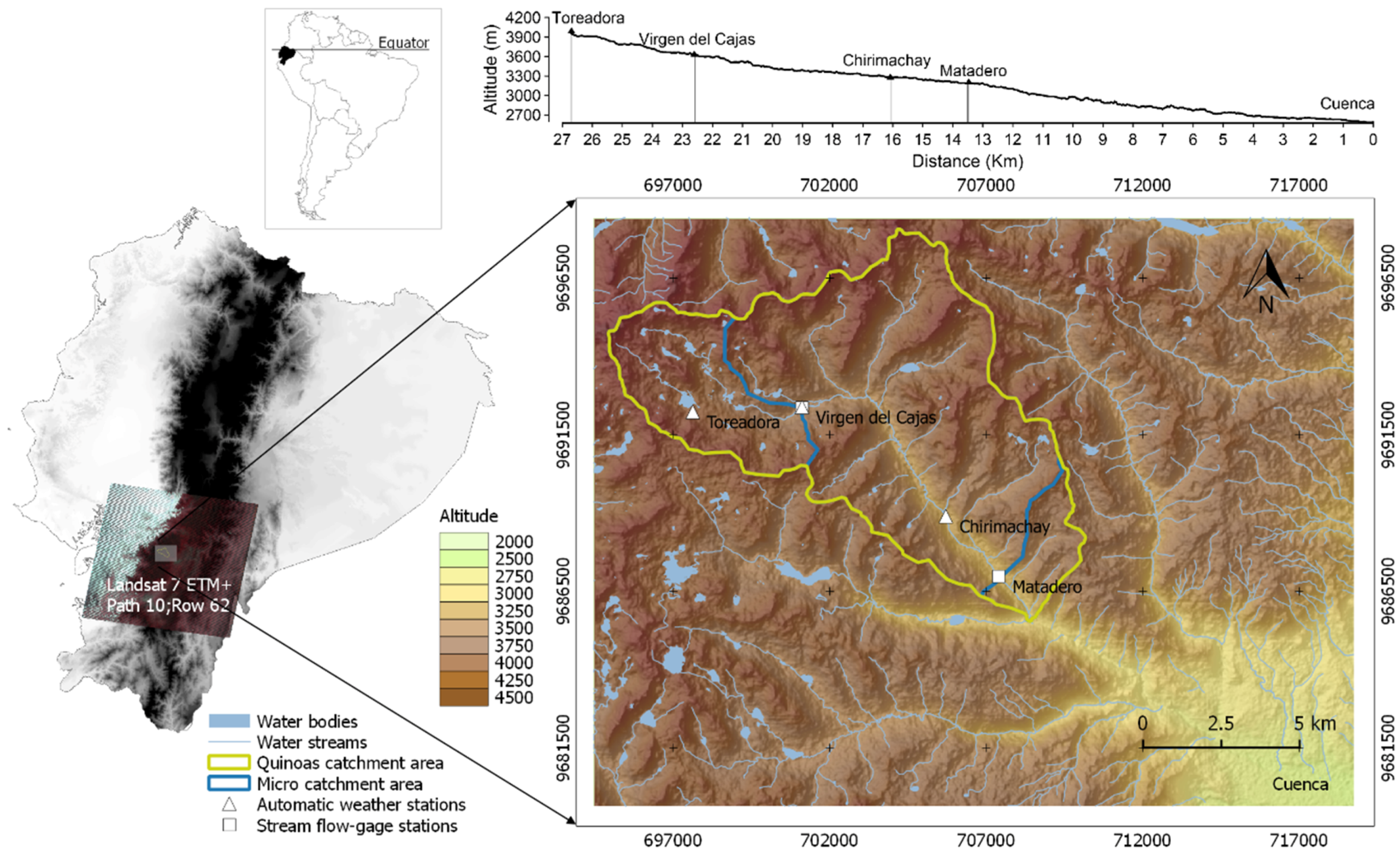
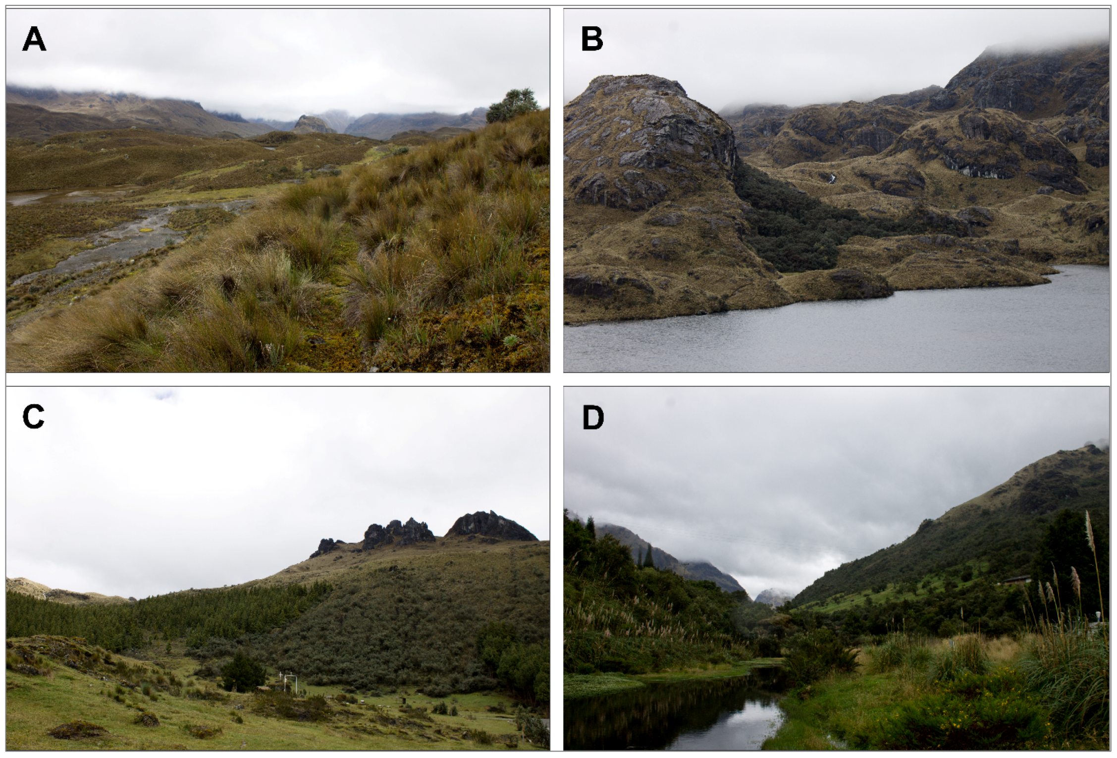
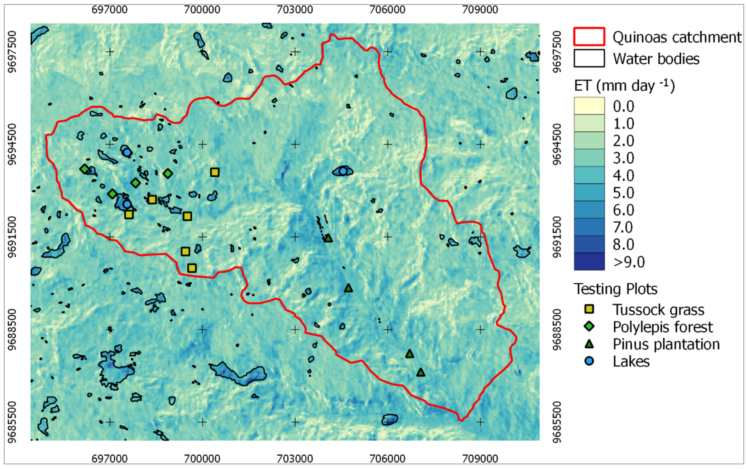
2.1. Study Area

Our study area is a páramo catchment exposed to the east mountainside of the Andes (2800 to 4250 masl) in southern Ecuador [64]. The climate of this region is mainly influenced by the continental air masses (moisture-laden) from the Amazon basin, to a lesser degree by the Inter Tropical Convergence Zone (ITCZ) fluctuations and in a few cases by dry cool air masses from the west (Humboldt current influence). Consequently, steady low temperatures and a prevalent convective and orographic cloud formation occur [65,66,67]. Although the Amazonian air masses tend to lose a high percentage of humidity due to condensation over the eastern lower flanks of the cordillera, annual precipitation totals between 800 and 1500 mm are common in the Andean highlands [68]. Hence, the páramo ecosystems have a surplus of water, constantly nourished by rainfall events and drizzle, as well as a slight fog interception [69].

In this region, the Quinoas catchment (94.1 km²) plays a significant role as a headwater catchment inside of the Cajas Massif, a UNESCO World Biosphere Reserve [70]. This catchment is located in the Paute River, a tributary of the Santiago River, which in turn is part of the Amazon basin. In the inter-Andean basin [71] below the páramo, more than 580,000 inhabitants benefit from the water supply from Quinoas and other neighboring catchments. Besides human consumption, agriculture, industrial activities and hydropower generation are supported by this abundant resource [72]. The catchment is mostly shaped by glacial landforms with slopes that usually range from 0% to 45%. Predominant soil types according to the FAO soil classification system are andosols and histosols [73], with a very high content of organic matter (30% and 60%, respectively) and a field capacity that ranges between 0.39 and 0.90 cm³·cm⁻³ (mean = 0.64) [74,75,76]. Wetlands and small lakes are important elements in the highlands.

Prevailing vegetation is tussock grass (Calamagrostis sp. and Festuca sp.), which covers more than 70% of the territory and coexists with cushion plant patches (e.g., Plantago sp., Valeriana sp. and Gentiana sp.), small forest patches of Polylepis sp. and Gynoxys sp. (<5%) and low shrubs, like Weinmannia sp. and Buddleia sp., among others [77,78]. Mid and low valley areas of the catchment (<3000 masl) are covered by sub-páramo (dominated by shrubs and grasses), upper Andean forest and grasslands with some areas afforested with Pinus patula sp. (25%). Andean tussock grasses and most of the native vegetation are perennial due to the slight seasonality [79,80,81]. Figure 1 shows the location of the study area, including topographic information, and Figure 2 shows predominant vegetation types in the catchment.

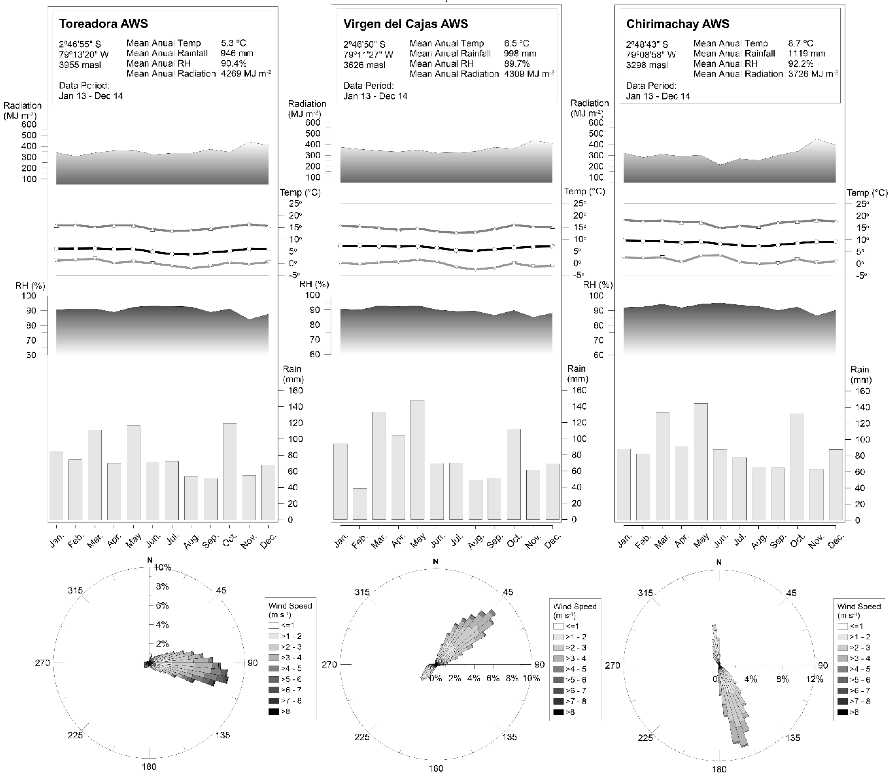
2.2. Weather and Stream Flow-Gage Stations

Three automatic weather stations (AWSs) and two stream flow-gage stations were installed in the catchment (details are in Figure 1 and

Table 1. Location of weather and stream flow-gage stations and typical vegetation cover in the surrounding area.

Station	Latitude and Longitude (UTM)	Elevation (masl)	Vegetation Type and Approximate Height
Toreadora 1	9692227.1; 697618.7	3955	Tussock Grass (“Pajonal”) (0.40 m)
Virgen del Cajas 1,2	9692382.2; 701110.7	3626	Mixed High Grass (0.40 m)/Low Grass (0.15 m)
Chirimachay 1	9688895.5; 705703.9	3298	Mixed: High Grass (0.40 m)/Native Subalpine and Forest (8 m)
Matadero 2	9686975.5; 707391.7	320	Mixed: High Grass (0.40 m)/Native Subalpine and Forest (>8 m)

¹ Automatic weather stations (AWSs); ² stream flow-gage station.

).

Meteorological and stream flow-gage data were collected every 5 min during 2013 and 2014 with a quality assessment [82]. Stream flow-gage datasets were available from July 2013 to June 2014.

Table 2. List of sensors used in the study.

Variable	Sensors	Unit	Accuracy	Time Resolution
Air Temperature/Relative Humidity 1,2	Campbell CS-215 + Radiation Shield	°C/% RH	±0.3 °C/±2% RH	5 min
Wind Speed and Direction 1	Met-One 034B Wind Set	m·s−1	±0.11 m·s−1	5 min
Pressure 1,2	Vaisala PTB110 Barometer	hPa	±0.3 hPa	5 min
Solar Radiation 1	Campbell CS300 Pyranometer	W·m−2	±5% daily total	5 min
Rainfall 1	Texas TE525MM Rain Gage	mm	±1%	5 min
Water Level 2	Campbell SR50A-L Sonic Ranging Sensor	m	±0.025 m	5 min

¹ At AWSs: Toreadora, Virgen del Cajas and Chirimachay; ² at stream flow-gage stations: Virgen del Cajas and Matadero.

and Figure 3 describe the deployed sensors and the meteorological data.

According to Figure 3, there is no significant temperature seasonality. However, considerable changes occur in the diurnal course. The average variability of the diurnal temperature range is 8.7 °C (average daily Tmax = 17.8° and Tmin = 1.8°) for all AWSs sites. Wind speed varies seasonally, with mean daily values of 3.0, 2.0 and 1.9 m·s⁻¹ from June to September and 1.9, 1.5 and 1.6 m·s⁻¹ for the rest of the year for Toreadora, Virgen del Cajas and Chirimachay, respectively. Likewise, daily total solar radiation also shows a light seasonal pattern, with average values of 13.9, 13.8 and 13.8 MJ·m⁻²·day⁻¹ from November to December and 11.3, 11.3 and 9.7 MJ·m⁻²·day⁻¹ for the rest of the year. Increased radiation in November leads to a decrease in relative humidity. In the same way, rainfall can be characterized by a bimodal pattern with a peak between March and May and another in October. The same rainfall regimes for the study area and for the inter-Andean basin were also reported by Célleri et al. [83].

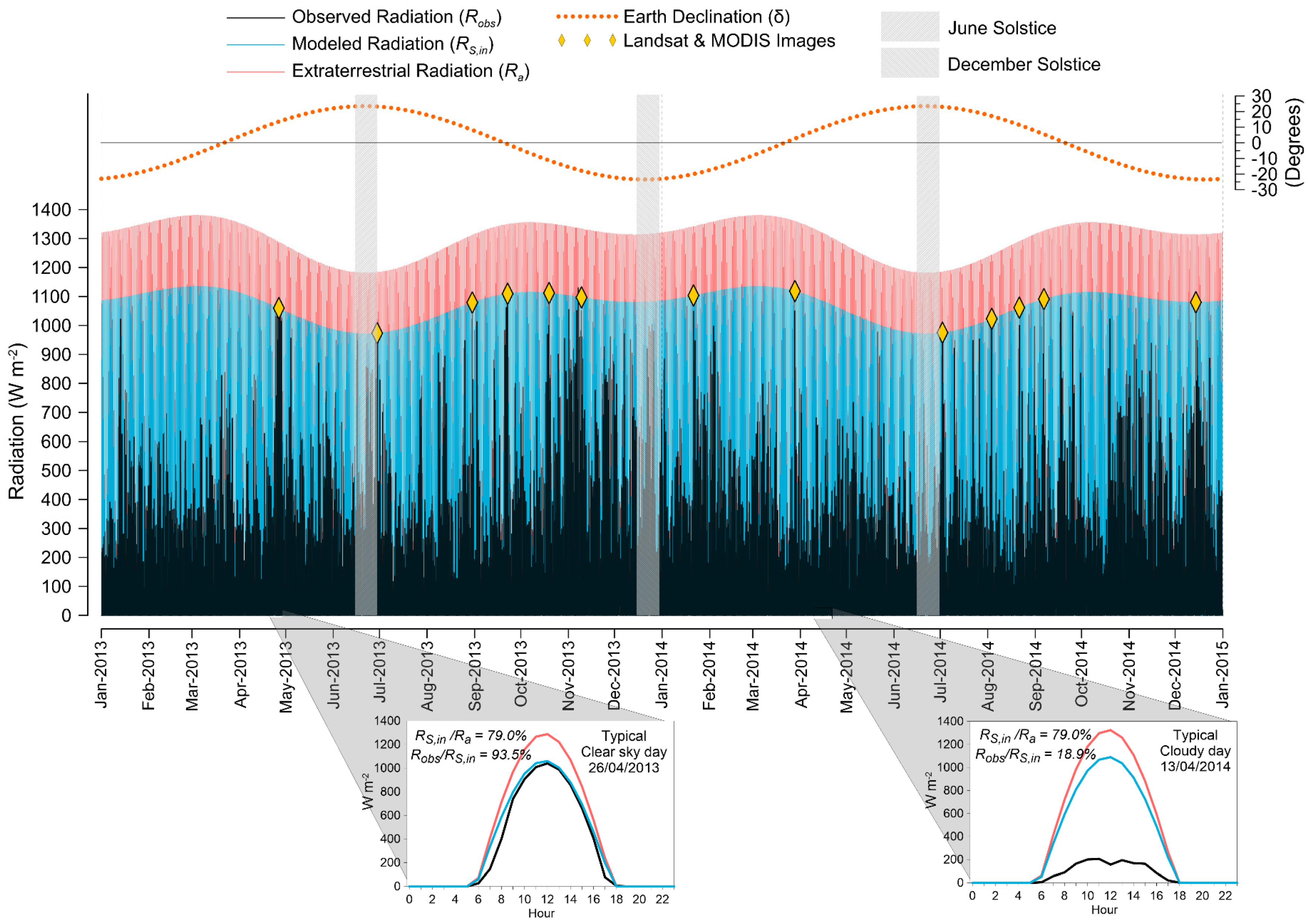
2.3. Landsat and MODIS Imagery

For the period April 2013 to December 2014, six Landsat 7 ETM+ SLC-off (scan line corrector off) scenes (30-m resolution) were obtained from the USGS Earth Explorer Nine cloud-free MODIS-Terra images (Level 1, 500-m resolution) were acquired from the Land Processes Distributed Active Archive Center (LP DAAC). MODIS-Terra data were selected considering sensor view angles <20° in order to avoid pixel deformation [36]. Finally, monthly MOD16 Evapotranspiration data (1000-m resolution) were taken from The Numerical Terradynamic Simulation Group (NTSG-University of Montana). Although optical satellite imagery is normally contaminated by frequent cloud cover over the Andes of Ecuador, especially in the southern Cordillera, all images used were hardly affected by clouds (

Table 3. Landsat and MODIS imagery for the study area.

Landsat 7 ETM + SLC-off Scene ID	Date	Path/Row	Cloud and Cloud-Shadow over the Quinoas Study Area * (%)
LE70100622013116EDC00	26 April 2013	10/62	0.0
LE70100622013180EDC00	29 June 2013	10/62	<9.4
LE70100622013292EDC00	19 October 2013	10/62	<12.1
LE70100622014087EDC00	28 March 2014	10/62	<9.5
LE70100622014183EDC00	2 July 2014	10/62	<12.5
LE70100622014215EDC00	3 August 2014	10/62	<38.0
MODIS-Terra Scene ID	Date	Tile Covering	Cloud and Cloud-Shadow over the Quinoas Study Area * (%)
MOD02HKM.A2013118.1530	28 April 2013	H10/V9	<5.0
MOD02HKM.A2013242.1555	30 August 2013	H10/V9	<3.0
MOD02HKM.A2013265.1600	22 September 2013	H10/V9	<30.0
MOD02HKM.A2013313.1600	9 November 2013	H10/V9	<8.0
MOD02HKM.A2014021.1555	21 January 2014	H10/V9	<35.5
MOD02HKM.A2014087.1540	28 March 2014	H10/V9	<30.9
MOD02HKM.A2014233.1530	21 August 2014	H10/V9	<20.0
MOD02HKM.A2014249.1530	6 September 2014	H10/V9	<5.0
MOD02HKM.A2014348.1600	14 December 2014	H10/V9	<2.5
MOD16 Global ET Product	Date	Tile Covering
MOD16A2 monthly imagery	January 2013 to December 2014	H10/V9

* Identified before the mosaicking procedure.

).

2.4. Pre-Processing of the Images

First, a radiometric correction for the Landsat and MODIS images was applied using the method recommended by Allen et al. [24] and Tasumi et al. [84]. The typical Landsat 7 SLC-off banding effect affected less than 2.3% of the image cover for our study area (due to its location in the center of the images with path/row = 10/62). Nonetheless, a gap filling correction was done to correct this problem using a focal analysis technique [85]. Finally, a mosaicking filling process was applied for the partially cloudy images. The latest was conducted using the FMASK algorithm for cloud and shadow detection [86], as well as a time-weighted interpolation technique recommended by Kjaersgaard et al. [87]. This process is explained in detail in the Supplementary Information of this paper. For the topographic correction in METRIC, we used the GDEM ASTER v2 digital elevation model (DEM) (30-m resolution), which was obtained from the NASA Land Processes Distributed Active Archive Center [88,89]. For the development of surface roughness maps, a land use/land cover map (LULC) was obtained from the Geoportal database of the Ministerio del Ambiente del Ecuador [90].

2.5. METRIC Model Implementation

METRIC delivers the instantaneous latent heat flux on a pixel-by-pixel basis as a residual of the subtraction of the soil and sensible heat fluxes from the available net radiation. METRIC includes a calibration procedure using inverse modeling at extreme climatic conditions where sensible heat fluxes are calibrated to wet and dry anchor pixels [24]. Figure S1 in the Supplementary Information of this paper shows the implementation flowchart of the METRIC model with Landsat and MODIS imagery, hereinafter called METRIC_L and METRIC_M, respectively. We used ERDAS Imagine™ and R software to implement the model.

2.5.1. METRIC Landsat-Based Implementation

A detailed explanation of the equations used in METRIC_L is given by Allen et al. [24] and also is shown in the Supplementary Information of this paper. The latter also included specific calibrations of the model implementation for Landsat imagery considering the following:

(i)

The incoming shortwave radiation was calculated considering terrain slope and aspect corrections for our location [24,91].

(ii)

The albedo was calculated according to [84].

(iii)

The emissivities were computed using the approach of Tasumi [92].

(iv)

LAI was derived from [93] and computed using the Soil-Adjusted Vegetation Index (SAVI) with a local calibration of the soil brightness-dependent factor (L) [94].

(v)

The surface temperature was estimated according to [95,96].

(vi)

Soil heat flux was calculated using the approach of [97,98].

(vii)

Sensible heat flux was calculated according to [24], where the roughness length values were assigned using a land use and land cover map (LULC) and specific values for the biome of the páramo [52,90,99,100].

(viii)

We implemented the method recommended by [53] for an adjustment of roughness length, z_om, a correction of wind speed for mountainous effects and a specific calibration of the temperature lapse rate for each image.

(ix)

Once radiation, soil and sensible fluxes were calculated, we obtained latent heat as the residual of the balance and subsequently the instantaneous ET [24], then converted it to a daily basis using the approach recommended by [24,101].

(x)

Cloud-contaminated pixels were previously assessed according to [24,37,86,87,102].

(xi)

Finally, ET on a daily basis was obtained applying a correction for solar radiation variability over sloping terrain [54], and monthly ET was calculated according to [38].

2.5.2. METRIC MODIS-Based Implementation

The METRIC_M implementation follows the same method as Landsat imagery, except for modifications in specific intermediate components and the use of a linear correlation of the reference evapotranspiration fraction (ET_rf) and the Normalized Difference Vegetation Index (NDVI) to assist in the selection process of the cold and hot pixels in accordance with the methodology of Trezza et al. [36]. The input imagery products we used were MOD02HKM v5 (calibrated radiances), MOD11_L2 v5 (land surface temperature), MOD03 (geolocation fields) and MOD35 (cloud mask). To obtain net radiation, we used the same methodology as METRIC_L with the following exceptions: albedo for MODIS_M was calculated by integrating the at-surface reflectances from Bands 1 to 7 of the MOD02 product [84]; surface temperature was obtained from the MODIS surface temperature product MOD11_L2; to obtain LAI, we applied the relationship between LAI-NDVI for different biomes described in the MODIS LAI backup method [103]; for our study, we calculated a linear relationship between the ET_rf and NDVI (previously obtained in the METRIC_L implementation) and aggregated it to the MODIS scale. According to a similar statistical approach by Allen et al. [104], we selected 20% of the coldest pixels from an NDVI population with the 20% highest values to obtain a local site calibrated relationship as shown in Equation (1).

$$\begin{gathered} E{T}_{r}f=0.804\times NDVI+0.289 ; \text{for} NDVI< 0.75 \\ E{T}_{r}f=1.05 ; \text{for} NDVI\ge 0.75 \end{gathered}$$

(1)

In the same way as in METRIC_L, we selected the hot pixels considering candidates with low vegetated pixels, relative high temperature and homogeneous terrain. A similar statistical-based approach was used. Cloud masking was performed using the MOD35 (cloud mask) product from USGS [105], and an interpolation for cloud masked images. Finally, the calculation of daily and monthly ET was carried out in a similar way as the METRIC_L implementation.

2.6. Analysis of the METRIC_L and METRIC_M Retrievals

In order to analyze the variability of daily ET according to the predominant vegetation of the study site, we selected and classified testing plots with homogeneous land cover. The selected plots in the ET maps were classified as follows: (i) tussock grass (6 sites in the head of the catchment); (ii) Polylepis sp. forest patches (4 sites in the high and mid locations); (iii) Pinus sp. forest plantations (4 in the lowlands); and (iv) water bodies (3 small lakes in the uplands). The plots had at least 500 × 500 m of properly identified biome during ground truth fieldwork campaigns. Polylepis plots are usually neighboring water bodies, and Pinus plots are mostly located in steep terrain. Daily time series of the ET maps were statistically analyzed (using mean, maximum and standard deviation) from one high radiation month (November) and one typical rainy month (April) in order to compare extreme situations. In addition to this, ET_rf (which is equal to a crop coefficient at the reference alfalfa basis according to Allen et al. [24]) retrieved METRIC_L and METRIC_M for the tussock grass sites were compared to literature values of grass-based crop coefficient (K_c) obtained by applying a conversion value (K_ratio) according to Allen et al. [106]. The method to obtain K_ratio is described in the Supplementary Information of this paper.

2.7. Comparison of METRIC Retrievals with MOD16 Product

METRIC_L and METRIC_M monthly ET retrievals were resampled (using nearest-neighbor interpolation) to a 1000-m resolution and were compared to the MODIS ET (MOD16) monthly product for the May 2013 to July 2014 period. The monthly MOD16 HDF archives were processed according to Mu et al. [107]. We used histogram-frequency analysis and the Kolmogorov–Smirnov distribution test to compare monthly ET maps for each product.

2.8. Validation of METRIC Retrievals with ET from the Water Balance

ET was directly inferred from the water balance as a difference between total precipitation and discharge (i.e., ET = P − Q) in two nested micro catchments inside the Quinoas catchment (areas of 19.5 and 87.2 km², respectively; see Figure 1 for the location). This approach was used because no evidence of groundwater contribution to discharge has been found in previous studies in the páramo sites of Ecuador [74,108]. Discharge data from the stream flow-gage stations of Virgen del Cajas and Matadero were used to calculate the runoff and runoff coefficients (i.e., Q/P) of each micro catchment. We applied the Manning equation [109] to convert water-level data into flow rates. A discharge vs. water-level analysis was conducted with constant-rate-based calibrations of stream flow measurements applying the salt-dilution technique [110,111]. Precipitation for the area was averaged using the Thiessen polygon method for the rain gauges data of the AWSs. A validation analysis of METRIC_L and METRIC_M retrievals with ET from the water balance was conducted using mean bias error (MBE), root mean square error (RMSE) and percent mean bias error (%MBE) according to Equations (2) to (4):

$$\text{MBE}=\frac{1}{n}{\displaystyle \sum }_{i=1}^n\left(E{T}_{\text{METRIC}/\text{MOD}16}-E{T}_{WB}\right)$$

(2)

$$\text{RMSE}=\sqrt{\frac{1}{n}{\displaystyle \sum }_{i=1}^n{\left(E{T}_{\text{METRIC}/\text{MOD}16}-E{T}_{WB}\right)}^2}$$

(3)

$$\%\text{MBE}=\frac{1}{n}{\displaystyle \sum }_{i=1}^n\frac{\left(E{T}_{\text{METRIC}/\text{MOD}16}-E{T}_{WB}\right)}{E{T}_{WB}}\times 100$$

(4)

where $E{T}_{\text{METRIC}/\text{MOD}16}$ is the monthly ET value of METRIC_L, METRIC_M or MOD16. $E{T}_{WB}$ is the monthly value of ET from the water balance. Finally, n is the number of months. In this analysis, we included the MOD16 ET product for comparative purposes against METRIC retrievals.

3. Results and Discussion

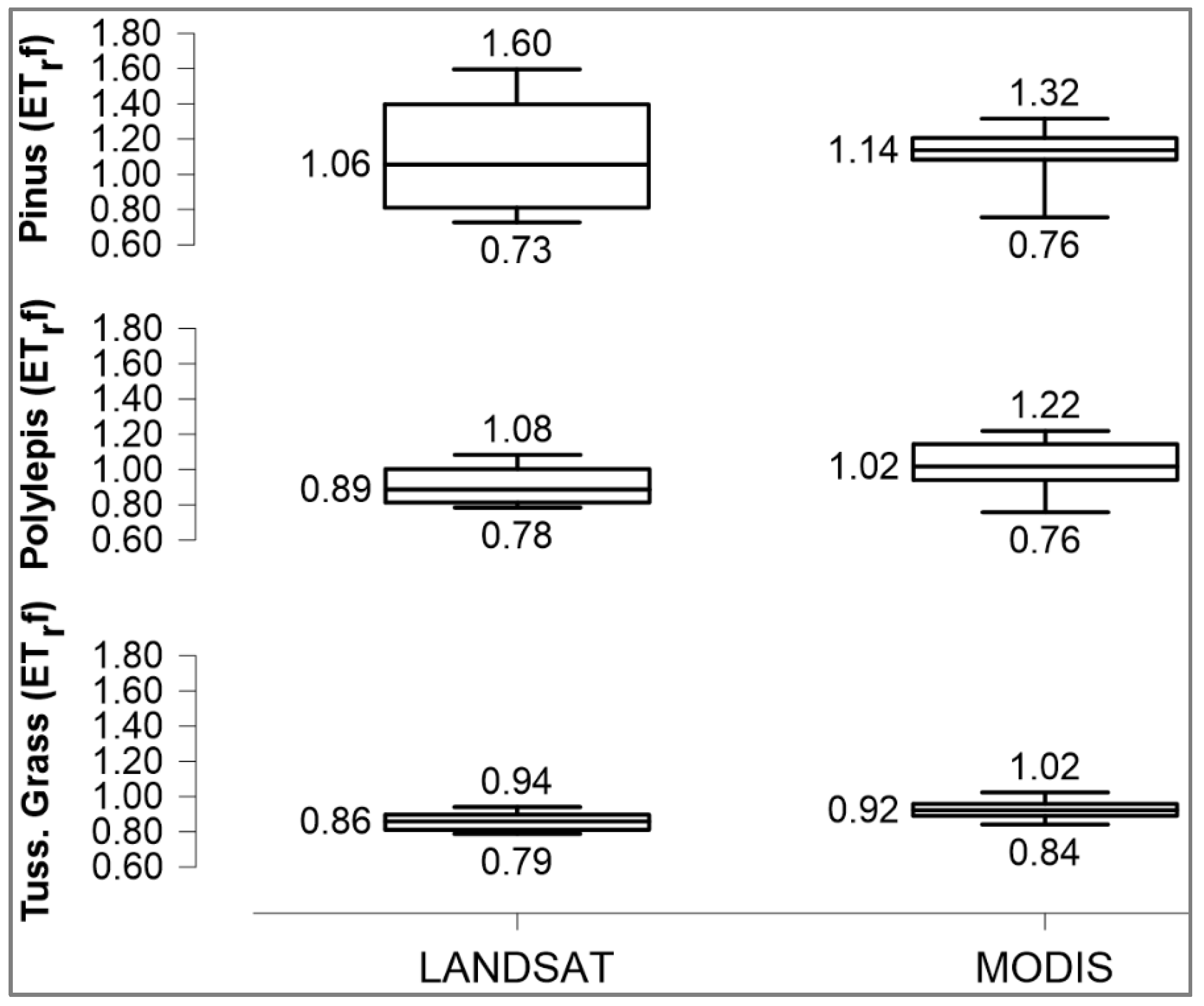
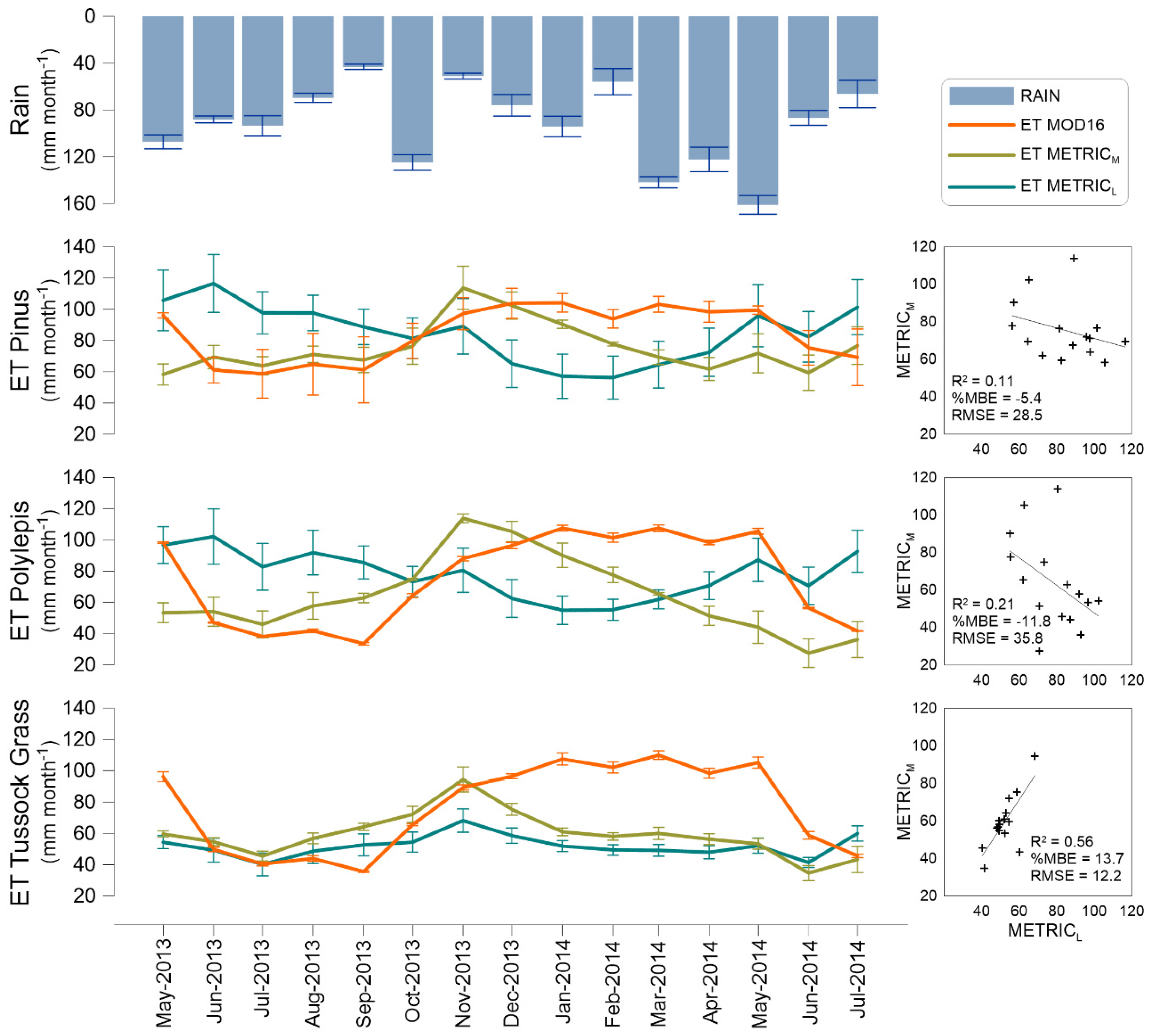
3.1. Reference Evapotranspiration Fraction (ET_rf) and Crop Coefficient (K_c)

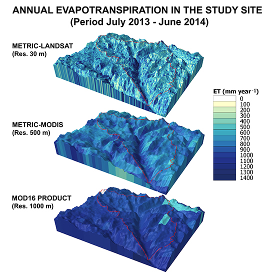
The ET_rf values for the three vegetated covers (testing plots) are illustrated in the boxplots of Figure 4 for the study period. We observe that METRIC_M ET_rf values were slightly higher than those obtained with Landsat. Trezza et al. [36] reported similar values of ET_rf for Landsat retrievals, but lower values for MODIS over high vegetation in the Middle Rio Grande valley of New Mexico. The differences in the medians between both products were 0.06, 0.13 and 0.08, respectively, for tussock grass, Polylepis and Pinus. The variation of ET_rf for the mentioned vegetation types can be attributed to the following factors: (1) the proximity of the Polylepis plots to water bodies and wetlands; and (2) the MODIS thermal band (MOD11-LST, 1000-m resolution) can be compromised by neighboring effects (especially in the steep terrain of Pinus plantations). The lower ET_rf variation for tussock grass sites was attributed to the relative surface thermal homogeneity; however, for the MODIS product, this variation probably was affected by the coarse resolution of its thermal band.

In order to compare the ET_rf values of the tussock grass to others reported in similar studies, we multiplied them by the K_ratio = 1.143 (calculated in an annual period). This value permitted converting ET_rf into an equivalent grass-based crop coefficient (K_c) as mentioned above. The equivalent range obtained for METRIC_L was 0.90–1.07. These values were closer to those obtained in highland irrigated meadows of northern Portugal (K_c = 0.88–0.89) [41] and to those reported for irrigated pastures in the lowlands of Galicia (K_c = 1.05) [112]. For METRIC_M, the equivalent range of K_c was 0.96–1.17. The latter retrievals were higher than Landsat values, which is probably due to the coarse resolution of the MODIS product and the heterogeneous vegetation cover within a single pixel. In addition, our results showed higher K_c than those reported by Buytaert et al. [81]: K_c = 0.42 for tussock grass and K_c = 0.95 for interfered areas in a field-scale study of páramo catchments. Our ET_rf and, thus, K_c estimations were supported by the evidence of no water stress and a constant humid condition of the soil.

3.2. 24-h ET Maps

Figure 5 presents an ET map for 19 October 2013 corresponding to the Landsat image of that cloud-free day. The testing plots are also marked in the map.

As thermally expected, lower ET values generally occurred in the crests, while higher ET values were found in the valley. The map shows that ET consistently decreases as altitude increases. The highest values were observed over water bodies and densely-vegetated areas, especially over the mountain forests and the riparian vegetation. The ET derived from the high vegetation in the northeast-facing slopes of the center valley is noticeable, particularly due to the amount of radiation in this month and the aspect/declination of these slopes. As expected, land cover directly impacts the amount of ET of the map. Daily ET statistics of METRIC_L and METRIC_M for single relatively dry and humid months in the testing plots are shown in

Table 4. METRIC_L and METRIC_M ET average daily values (mm·day⁻¹) according to site type.

	n	November 2013 (High Radiation Month)			April 2014 (Low Radiation, Rainy Month)			Period. Diff.
		Mean	Max	SD	Mean	Max	SD
ET METRICL (mm·day−1)
Tussock grass sites	6	2.27	3.56	0.63	1.64	2.76	0.47	−0.63
Polylepis sp. forest sites	4	2.68	4.46	0.84	2.36	3.79	0.72	−0.32
Pinus sp. forest sites	4	2.83	4.37	0.85	2.44	3.83	0.72	−0.39
Water body	3	4.37	7.01	1.33	4.46	7.02	1.34	0.09
ET METRICM (mm·day−1)
Tussock grass sites	6	3.31	5.07	0.88	1.90	3.44	0.54	−1.41
Polylepis sp. forest sites	4	3.98	5.87	1.00	1.69	3.41	0.53	−2.29
Pinus sp. forest sites	4	3.55	4.93	0.94	1.96	2.93	0.52	−1.59
Water body	3	3.66	5.32	0.95	2.06	3.68	0.60	−1.6
METRIC Difference (means and max.) (mm·day−1)
Tussock grass sites		1.04	1.51		0.26	0.68
Polylepis sp. forest sites		1.3	1.41		−0.67	−0.38
Pinus sp. forest sites		0.72	0.56		−0.48	−0.9
Water body		−0.71	-1.69		−2.4	−3.34

* Mean = mean of daily ET; Max = maximum of daily ET; SD = standard deviation in the period; Period. Diff. = difference of the means between periods; n = 30 days for November and April.

.

Table 4 shows that daily averages of METRIC_L generally increase from tussock to trees to water bodies similarly to applications of METRIC and SEBAL over riparian vegetation [36,41]; for METRIC_M, this finding is not noticeable, mainly due the lack of spatial fidelity of the model considering the heterogeneity of our study area. Both METRIC_L and METRIC_M daily results revealed differences between the relatively dry and humid months, with ET values in November 2013 higher than in April 2014 for all vegetated-sites, with the exception of water bodies in METRIC_L. This was in agreement with the local climate (Section 2.2), where increments of solar radiation cause a reduction in relative humidity and the differences between both periods were wider for METRIC_M than for METRIC_L. We presume this finding is associated with an increased sensitivity of the METRIC_M model when rain events occur, as previously reported by Ruhoff et al. [113]. Mean ET values for tussock grass are in agreement with those reported by Pôças et al. [41] for grasslands in northern Portugal.

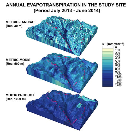
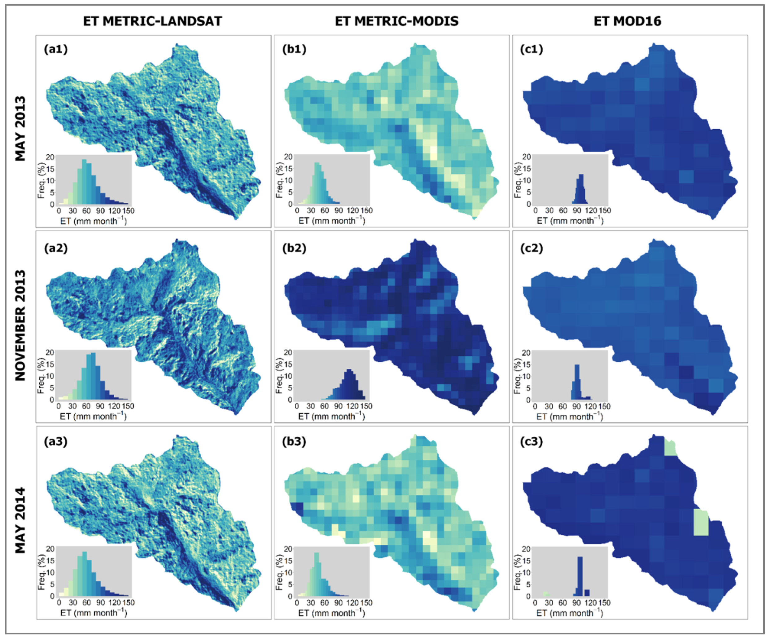
3.3. Monthly ET Retrievals and Comparison with MOD16 ET

Figure 6 shows the monthly METRIC_L, METRIC_M ET and monthly MOD16 ET product comparison for May 2013 (Figure 6a1,b1,c1), November 2013 (Figure 6a2,b2,c2) and May 2014 (Figure 6a3,b3,c3), respectively. For the METRIC outputs, changes in ET presented a corresponding pattern between wet and dry periods. METRIC_L showed lower ET (mean = 68.9 mm, SD = 23.0 mm) in the driest month, while higher values were found for METRIC_M (mean = 110.1 mm, SD = 16.5 mm) and MOD16 ET (mean = 89.9 mm, SD = 5.4 mm) for the same month. Distributions of ET values in humid months (May 2013 and May 2014) were similar between METRIC_L and METRIC_M with Kolmogorov–Smirnov (KS) distances of 0.080 and 0.086, respectively. The same observation does not hold for MOD16 ET (KS value of 0.564 for the same months), which revealed that distributions between these products were different. The standard deviations were considerably higher for METRIC products than for MOD16, probably due to the capability of the model to capture the land cover and topography heterogeneity.

The noticeable difference of the METRIC retrievals in November 2013 revealed a tendency of the METRIC_M model to overestimate ET when compared to METRIC_M and MOD16 in this month. This could be attributed to the model’s inability to reproduce the predominant high-moisture conditions of the páramo during this relatively less wet period and also to the errors in the estimation of net radiation due the limited capacity of the surface temperature input (MOD11_L2) to account for cloudy conditions in a high radiation month. This has also been reported by Ruhoff et al. [113] for a SEBAL implementation in Brazil. On the other hand, we observed lower values of METRIC_M for May 2013 and 2014; this indicated that the sensitivity of the model is clearly affected by rainfall and radiation seasonality (moisture and cloudiness increased). The ET variability of the complete period will be explained further.

Additionally, ET values in May were higher on northeast-facing slopes of the center of the valley (center of Figure 6a1,a3). This effect is attributed to the METRIC radiation sub-model due to a combination of two factors: (1) the seasonal variation of the declination of the Earth; and (2) the aspect angle of the area. The northeast-facing slope of this part of the valley has an aspect angle of 24.2° (considering the east-west horizontal) and an average slope of 45.2°; hence, for months with a high incident angle of the Sun (due to the June solstice), the impact is significant.

In Figure 7, we observe the typical oscillation in the Earth declination angle (δ). This parameter ranges for May from +14.8° to +21.8° and for November from −14.19° to −21.5°. Thus, the incident radiation increases ET over the northeast-facing slopes of the valley in the humid months. This increase is clearly reduced in November (December solstice), where the southwest-facing slope of the valley receives more radiation. The acquisition time of the Landsat imagery is around 10:30 and for MODIS between 10:30 and 11:00 (local time), when (in June) the northeast slopes are normal to the Sun. In addition, the dense forest vegetation in this part of the valley strengthens this effect by increasing the NDVI. It is important to mention that mountain shadows are not accounted for in the 24-h radiation algorithm [54]. In addition, Ramsay [114] stated that east-facing slopes receive more sunlight in páramo ecosystems, mainly due to differences in rainfall on lee and windward slopes and cloudiness occurrence during the afternoon on west-facing slopes.

Figure 7 also reveals the marked difference between the modeled and observed radiation (the latest retrieved from the AWSs pyranometers) with an hourly time step. The Landsat and MODIS image dates used in the study are also depicted in the figure.

The analysis of Figure 7 determines that: (1) the radiation sub-model was able to reduce 21% of the extraterrestrial radiation (R_a) considering clear-sky conditions; (2) the modeled radiation (R_S,in) constantly varied according to the Sun angle and elevation-related fluctuations of R_a and with the atmospheric transmissivity at cloud-free conditions; (3) when R_S,in was compared to ground-level radiation measurements (R_obs), good estimations were obtained only when clear-sky conditions prevailed (difference of 6.5% of R_obs). Given considerable cloudiness, the sub-model would overestimate radiation up to 81% of the R_obs, and this in turn would lead to an overestimation in ET.

Time series of METRIC_L and METRIC_M retrievals were compared to the MOD16 ET product and average rainfall from the AWSs; results are shown in Figure 8. Statistical comparison between METRIC estimations (i.e., coefficient of determination, R², percent mean bias, %MBE, and root mean square error, RMSE) are also included in the figure.

According to Figure 8, METRIC_L and METRIC_M for tussock grass showed a R² coefficient of 0.56. This can be attributed to the relative homogeneity of the vegetation and topographic characteristics of the plots. For the tussock grass sites (most representative vegetation cover in our area), an increment of ET in the last months of 2013 (October November, and December) and a clear reduction in the rainy-humid season (more visible for 2014 than for 2013) with a small error for the models retrievals were noticeable; however, for the Polylepis and Pinus sites, this finding is similar, but with a great temporal variability and significant errors for all products. The above-mentioned increment in ET is attributed to the reduction of the vapor pressure deficit (due to the increment of water in the atmosphere) and to a reduction in the incoming solar energy due to the reigning cloudy conditions in these periods. Positive bias (13.7%) and lower RMSE (12.2 mm·month⁻¹) were observed for tussock grass sites. Nonetheless, Polylepis and Pinus sites showed lower R² coefficients than tussock grass (0.21 and 0.11, respectively), as well as negative bias (−11.8% and −5.4%) and higher RMSE (35.8 and 28.5 mm·month⁻¹). This finding can be attributed to the lack of the spatial fidelity of METRIC_M when applied over heterogeneous vegetated areas in steep terrain.

MOD16 time series exposed an overestimation for November 2013 to June 2014; this was more evident for the tussock grass sites than the other vegetation covers. This finding reveals that MOD16 was not able to capture the diminishing of ET in this relatively humid period, in contrast to METRIC retrievals. A similar behavior was seen in May 2013. The rainy and high radiation month October 2013 slightly impacted ET to all models, unlike the longest annual rainy period. Overestimation of MOD16 has already been reported for the tropics in other studies [115,116,117]. We also calculated the %MBE and RMSE values for MOD16 when compared to METRIC_L outputs (tussock grass %MBE = 47.6% and RMSE = 36.0 mm·month⁻¹; Polylepis %MBE = 4.5% and RMSE = 38.7 mm·month⁻¹; and Pinus %MBE = 7.6% and RMSE = 31.6 mm·month⁻¹). Generally, bias and RMSE for MOD16 were higher than for METRIC. However, considering that tussock grass vegetation constitutes the most extensive area in our study site (>70%), a lack of METRIC accuracy in the forest land covers is understandable. Our results are what we expected due to the low representativeness of these land covers.

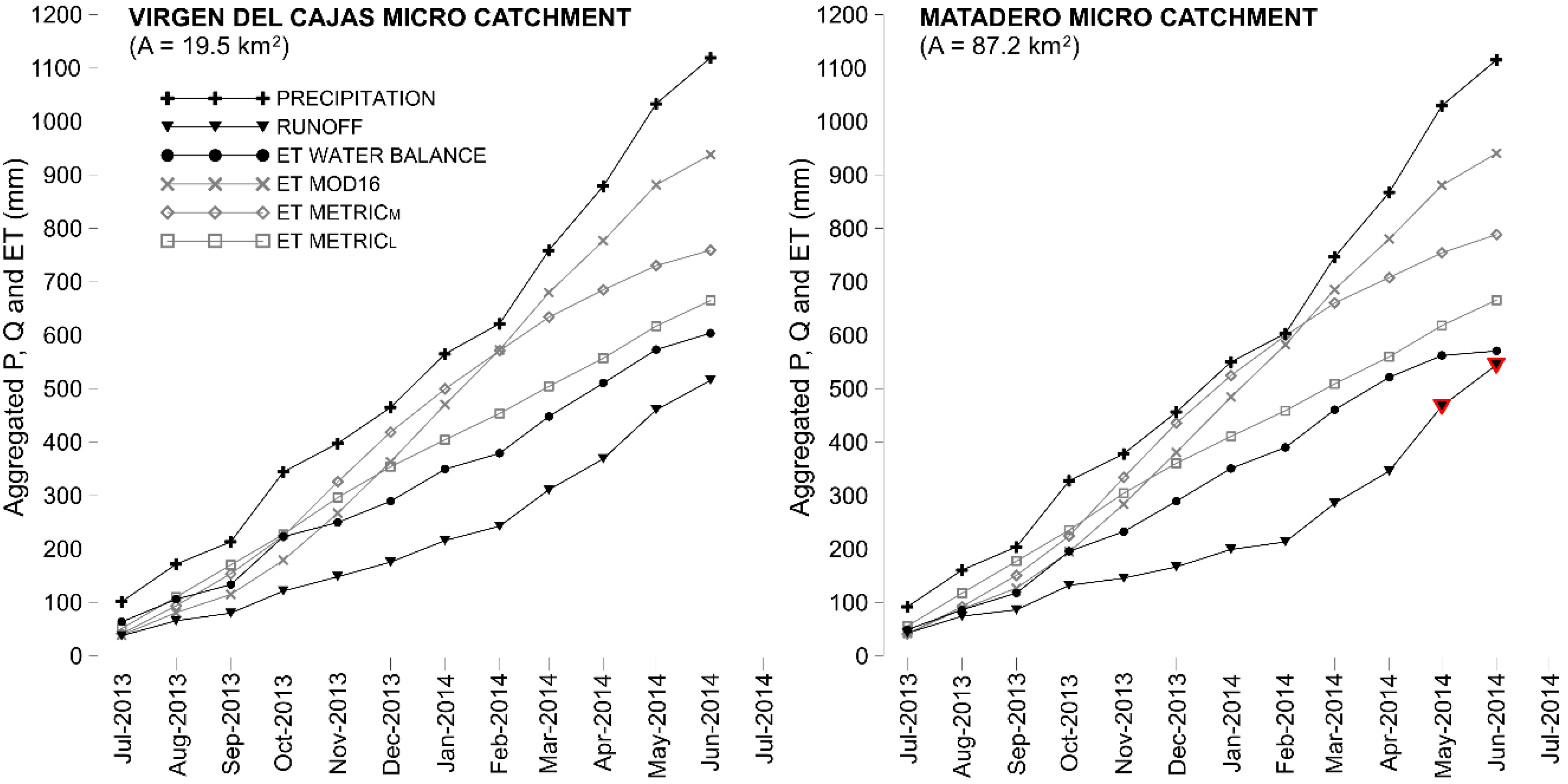
3.4. Validation with ET from the Water Balance

The runoff coefficients corresponding to our validation micro catchments were 0.46 for the Virgen del Cajas micro catchment (head of the basin) and 0.49 for the Matadero micro catchment (whole basin) for the data-available study period. These runoff coefficients were similar to those obtained by Mosquera et al. [6] for a small páramo catchment (A = 7.53 km²) located 35 km south of our study area and those reported by Crespo et al. [74] for a páramo micro catchment near the study area. Both reported studies have very similar biophysical conditions (i.e., soil type, vegetation and elevations) to the present study. The aggregated values for runoff (Q), precipitation (P) and residual ET for our study are depicted in Figure 9.

Figure 9 shows similar patterns for P, Q and ET for both micro catchments, although Matadero runoff shows a noticeable increment during rainy months. Mosquera et al. [6] determined that ET from the water balance is particularly sensitive to increments in runoff of páramo, especially in the lowest micro catchments (where land use change and non-native vegetation prevail), which was noticeable in May and June 2014. The validation approach demonstrated that METRIC_L ET aggregated values tend to align closer to the water balance ET, while the estimates of METRIC_M and MOD16 significantly overestimated it. The results of the monthly/annual statistical analysis are summarized in

Table 5. Comparison of METRIC_L, METRIC_M and MOD16 retrievals with ET from the water balance in the micro catchments (annual and monthly scale). For the micro catchments locations, refer to Figure 1.

	Virgen del Cajas Micro Catchment				Matadero Micro Catchment
	ET Water Balance	ET METRICL	ET METRICM	ET MOD16	ET Water Balance	ET METRICL	ET METRICM	ET MOD16
Annual Total (mm·year−1)	603.91	664.91	759.04	937.91	570.70	665.82	788.53	940.50
Annual Error (mm·year−1)		61.01	155.14	334.00		95.12	217.84	369.80
Percent Annual Error (%)		10.10	25.69	55.31		16.67	38.17	64.80
Monthly Mean (mm·month−1)	50.33	55.41	63.25	78.16	47.56	55.49	65.71	78.37
Monthly MBE (mm·month−1)		5.08	12.93	27.83		7.93	18.15	30.82
Percent Monthly MBE (%)		30.42	51.37	76.15		57.36	65.79	108.28
Monthly RMSE (mm·month−1)		22.02	33.06	41.69		21.23	30.61	39.03

.

Results in Table 5 reveal that annual statistics were better for the upland smaller micro catchment (Virgen del Cajas) than for the larger micro catchment (Matadero). This might be due to the relative homogeneity of páramo vegetation above 3500 masl, in contrast to the heterogeneous vegetation and steep topography observed in the mid and low valley. RMSE was slightly lower for the larger micro catchment (Matadero). METRIC_L retrievals showed annual and monthly differences of 10% and 30%, respectively, for the Virgen del Cajas micro catchment and 17% and 57%, respectively, for the Matadero micro catchment. Annual differences for METRIC_M estimates were two times higher for both micro catchments, and monthly %MBE was larger, as well. MOD16 retrievals showed the most significant differences for annual and monthly time steps in both micro catchments, where annual %MBE ranges from 55%~65%.

Monthly RMSE values were lower for METRIC_L when compared to METRIC_M and MOD16 for both micro catchments. We found that METRIC_L annual differences ranged within the absolute errors of annual/seasonal ET, which according to Karimi and Bastiaanssen [13] varied between 1% and 20%. In addition, Velpuri et al. [62] reported differences of 17 and 6 mm·month⁻¹ for MOD16 and the Operational Simplified Surface Energy Balance (SSEBop) model, respectively, in locations with an elevation >1500 masl in the southwestern United States.

In a comparative study between the water balance ET and SEBAL ET, an overestimation of 17% for the SEBAL ET retrievals was reported for a mountainous catchment in central Iran (semi-arid and cold conditions) [45]. Consequently, METRIC_L ET presented very good performance in comparison to the energy balance-based ET models reported in previous studies, in spite of the unsatisfactory performance of METRIC_M ET for our investigation. The main reason for the overestimation observed in both METRIC_L and METRIC_M ET retrievals can be attributed to the model limitation to estimate the diminished incoming radiation levels in the páramo (clearly noticeable in Figure 7). This was also reported by similar studies where the prevailing cloudy conditions represented a challenge when energy balance-based models were applied [113,118,119].

The overestimation of the incoming energy only affected the ET_rf calculations, in contrast to ET_r, which used the ground-level radiation measurements and was obtained via the ASCE-ERWI Standardized Reference Evapotranspiration Equation [101]. In addition, overestimation of aggregated daily or monthly ET for the páramo can be influenced by a stable daily temperature condition during long periods (more than a week) due to a decrease in relative humidity, especially in the absence of rain events [12]. For the above-mentioned reasons, the use of direct measurements of solar radiation and relative humidity in the páramo is crucial for ET_r calculations, which supports the findings of Córdova et al. [11].

4. Concluding Remarks

Our study demonstrated that spatially-explicit ET can be estimated for tropical páramo catchments using an energy balance-based approach for two remote sensing products and with a dynamic aggregation of the time series. The latter was possible when adequate topographic corrections and specific model adaptations were properly performed, as well as a systematic hot and cold pixel selection. In this way, we found anchor pixels with a sufficient temperature range for a successful application of METRIC in the páramo, which is similar to other studies conducted over non-water stressed vegetation and also in semi-arid climates [36,104]. However, model sensitivity to rainfall occurrence remains unknown and requires a deeper study into the benefit of a fine adjustment of the model, similarly to Singh et al. [120]. This has not been investigated in the Andes, mainly due the inexistence of in site flux measurements, like the Bowen ratio or eddy covariance, to obtain observed values of latent and sensible heat flux and, hence, actual ET.

The good performance of METRIC_L retrievals has been confirmed by the validation using catchment-scale runoff and precipitation data. Monthly and annual differences are around 30% and 10%, respectively, for METRIC_L, which points to a slight overestimation, as already expected based on similar studies [13,45]. However, this level of error is the minimum to be expected, considering that we cannot account for the uncertainty of the runoff and precipitation measurements. Nonetheless, we assume that the sensitivity of the model to vegetation and terrain heterogeneity is superior to the other products, considering the finer resolution of Landsat imagery and the terrain correction approach using a mid-high resolution elevation model.

Cloud cover conditions were not captured by the incoming radiation sub-model, and the corrections for modeled atmospheric transmissivity were insufficient to account for the strong cloudiness variability. For METRIC_M, we detected a lack of accuracy causing an overestimation of ET that can be attributed to its coarse scale. This overestimation was particularly related to the MODIS thermal band of a 1000-m resolution, which averaged sub-pixel heterogeneity and, thus, affected thermally-representative anchor pixels.

Despite the unsuitable results of METRIC_M, the local calibration of the ET_rf vs. NDVI function seems to be a feasible approach to retrieve near-real ET estimations in the páramo using MODIS imagery. In terms of water management, ET overestimation would lead to an underestimation of the runoff in the hydrological balance when data on stream flows are not available (i.e., only rainfall measurements and ET estimations available). For that reason, the local calibration of specific parameters in the model is a mandatory requirement to improve the accuracy of the ET maps, particularly when those spatial retrievals will serve as the input in hydrological studies. In our study, we also recognized the limitations of the method under a low availability of clear-sky images. Nevertheless, the applicability of this method over perennial vegetation covers (like the páramo grasslands and native evergreen forests) using a limited amount of images has been demonstrated with plausible results. Thus, METRIC_L showed high potential as a monitoring tool for the mountain páramos on an operational basis. Finally, the comparative analysis revealed that the global ET product MOD16 was rendered deficient for our study area, which emphasizes the importance of further refinement of this VI-ET model for applications in the tropical Andes.

Future work should pursue a more accurate validation of daily spatial ET retrievals with field-scale measurements (eddy covariance and porometry techniques) and also the study of similar water depletion key indicators, such as water use efficiency over this singular Andean ecosystem.

References

1. Pepin, N.; Bradley, R.S.; Diaz, H.F.; Baraer, M.; Caceres, E.B.; Forsythe, N.; Fowler, H.; Greenwood, G.; Hashmi, M.Z.; Liu, X.D.; et al. Elevation-dependent warming in mountain regions of the world. Nat. Clim. Chang. 2015, 5, 424–430. [Google Scholar] [CrossRef] [Green Version]
2. Krishnaswamy, J.; John, R.; Joseph, S. Consistent response of vegetation dynamics to recent climate change in tropical mountain regions. Glob. Chang. Biol. 2014, 20, 203–215. [Google Scholar] [CrossRef] [PubMed]
3. Mora, D.E.; Campozano, L.; Cisneros, F.; Wyseure, G.; Willems, P. Climate changes of hydrometeorological and hydrological extremes in the Paute basin, Ecuadorean Andes. Hydrol. Earth Syst. Sci. 2014, 18, 631–648. [Google Scholar] [CrossRef] [Green Version]
4. Vuille, M.; Bradley, R.S.; Werner, M.; Keimig, F. 20th century climate change in the tropical Andes: Observations and model results. In Climate Variability and Change in High Elevation Regions: Past, Present & Future; Springer: Houten, The Netherlands, 2003; pp. 75–99. [Google Scholar]
5. Vuille, M.; Franquist, E.; Garreaud, R.; Lavado Casimiro, W.S.; Cáceres, B. Impact of the global warming hiatus on Andean temperature. J. Geophys. Res. Atmos. 2015, 120, 3745–3757. [Google Scholar] [CrossRef]
6. Mosquera, G.M.; Lazo, P.X.; Célleri, R.; Wilcox, B.P.; Crespo, P. Runoff from tropical alpine grasslands increases with areal extent of wetlands. Catena 2015, 125, 120–128. [Google Scholar] [CrossRef]
7. Crespo, P.; Celleri, R.; Buytaert, W.; Feyen, J. Land use change impacts on the hydrology of wet Andean páramo ecocystems. In Proceedings of the Workshop Status and Perspectives of Hydrology in Small Basins, Goslar-Hahnenklee, Germany, 30 March–2 April 2009; IAHS Publications: Wallingford, UK, 2010; p. 336. [Google Scholar]
8. Thies, B.; Meyer, H.; Nauss, T.; Bendix, J. Projecting land-use and land-cover changes in a tropical mountain forest of Southern Ecuador. J. Land Use Sci. 2014, 9, 1–33. [Google Scholar] [CrossRef]
9. Balthazar, V.; Vanacker, V.; Molina, A.; Lambin, E.F. Impacts of forest cover change on ecosystem services in high Andean mountains. Ecol. Indic. 2015, 48, 63–75. [Google Scholar] [CrossRef]
10. Llambí, L.D.; Soto-W, A.; Célleri, R.; de Bievre, B.; Ochoa, B.; Borja, P. Ecología, Hidrología y Suelos de Páramos. Proyecto Páramo Andino; Universidad de Los Andes: Bogotá, Colombia, 2012. [Google Scholar]
11. Córdova, M.; Carrillo-Rojas, G.; Crespo, P.; Wilcox, B.; Célleri, R. Evaluation of the Penman-Monteith (FAO 56 PM) method for calculating reference evapotranspiration using limited data. Mt. Res. Dev. 2015, 35, 230–239. [Google Scholar] [CrossRef]
12. Córdova, M.; Carrillo, G.; Célleri, R. Errores en la Estimación de la Evapotranspiración de Referencia de una zona de Páramo Andino debidos al uso de datos Mensuales, Diarios y Horarios. Aqua-LAC 2013, 5, 14–22. [Google Scholar]
13. Karimi, P.; Bastiaanssen, W.G.M. Spatial evapotranspiration, rainfall and land use data in water accounting—Part 1: Review of the accuracy of the remote sensing data. Hydrol. Earth Syst. Sci. Discuss. 2014, 11, 1073–1123. [Google Scholar] [CrossRef]
14. Gowda, P.H.; Chavez, J.L.; Colaizzi, P.D.; Evett, S.R.; Howell, T.A.; Tolk, J.A. ET mapping for agricultural water management: Present status and challenges. Irrig. Sci. 2008, 26, 223–237. [Google Scholar] [CrossRef]
15. Liou, Y.A.; Kar, S.K. Evapotranspiration estimation with remote sensing and various surface energy balance algorithms—A review. Energies 2014, 7, 2821–2849. [Google Scholar] [CrossRef]
16. Allen, R.G.; Pereira, L.S.; Howell, T.A.; Jensen, M.E. Evapotranspiration information reporting: I. Factors governing measurement accuracy. Agric. Water Manag. 2011, 98, 899–920. [Google Scholar] [CrossRef]
17. Irmak, A. Evapotranspiration—Remote Sensing and Modeling; InTech: Rijeka, Croatia, 2011. [Google Scholar]
18. Kustas, W.P.; Norman, J.M. Use of remote sensing for evapotranspiration monitoring over land surfaces. Hydrol. Sci. J. 1996, 41, 495–516. [Google Scholar] [CrossRef]
19. Moran, M.S.; Jackson, R.D. Assessing the spatial distribution of evapotranspiration using remotely sensed inputs. J. Environ. Qual. 1991, 20, 725–737. [Google Scholar] [CrossRef]
20. Courault, D.; Seguin, B.; Olioso, A. Review on estimation of evapotranspiration from remote sensing data: From empirical to numerical modeling approaches. Irrig. Drain. Syst. 2005, 19, 223–249. [Google Scholar] [CrossRef]
21. Verstraeten, W.W.; Veroustraete, F.; Feyen, J. Assessment of evapotranspiration and soil moisture content across different scales of observation. Sensors 2008, 8, 70–117. [Google Scholar] [CrossRef]
22. Li, Z.-L.; Tang, R.; Wan, Z.; Bi, Y.; Zhou, C.; Tang, B.; Yan, G.; Zhang, X. A review of current methodologies for regional evapotranspiration estimation from remotely sensed data. Sensors 2009, 9, 3801–3853. [Google Scholar] [CrossRef] [PubMed]
23. Kalma, J.D.; McVicar, T.R.; McCabe, M.F. Estimating land surface evaporation: A review of methods using remotely sensed surface temperature data. Surv. Geophys. 2008, 29, 421–469. [Google Scholar] [CrossRef]
24. Allen, R.G.; Tasumi, M.; Trezza, R. Satellite-based energy balance for mapping evapotranspiration with internalized calibration (METRIC)—model. J. Irrig. Drain. Eng. 2007, 133, 380–394. [Google Scholar] [CrossRef]
25. Bastiaanssen, W.G.M.; Menenti, M.; Feddes, R.A.; Holtslag, A.A.M. A remote sensing surface energy balance algorithm for land (SEBAL): 1. Formulation. J. Hydrol. 1998, 212–213, 198–212. [Google Scholar] [CrossRef]
26. Norman, J.M.; Kustas, W.P.; Humes, K.S. Source approach for estimating soil and vegetation energy fluxes in observations of directional radiometric surface temperature. Agric. For. Meteorol. 1995, 77, 263–293. [Google Scholar] [CrossRef]
27. Su, Z. The Surface Energy Balance System (SEBS) for estimation of turbulent heat fluxes. Hydrol. Earth Syst. Sci. Discuss. 2002, 6, 85–100. [Google Scholar] [CrossRef]
28. Sun, Z.; Wang, Q.; Matsushita, B.; Fukushima, T.; Ouyang, Z.; Watanabe, M. Development of a simple remote sensing evapotranspiration model (Sim-ReSET): Algorithm and model test. J. Hydrol. 2009, 376, 476–485. [Google Scholar] [CrossRef] [Green Version]
29. Kustas, W.P.; Norman, J.M. Evaluation of soil and vegetation heat flux predictions using a simple two-source model with radiometric temperatures for partial canopy cover. Agric. For. Meteorol. 1999, 94, 13–29. [Google Scholar] [CrossRef]
30. Anderson, M.C.; Norman, J.M.; Diak, G.R.; Kustas, W.P.; Mecikalski, J.R. A two-source time-integrated model for estimating surface fluxes using thermal infrared remote sensing. Remote Sens. Environ. 1997, 60, 195–216. [Google Scholar] [CrossRef]
31. Morton, C.G.; Huntington, J.L.; Pohll, G.M.; Allen, R.G.; Mcgwire, K.C.; Bassett, S.D. Assessing calibration uncertainty and automation for estimating evapotranspiration from agricultural areas using METRIC. J. Am. Water Resour. Assoc. 2013, 49, 549–562. [Google Scholar] [CrossRef]
32. Carrasco-Benavides, M.; Ortega-Farías, S.; Lagos, L.; Kleissl, J.; Morales-Salinas, L.; Kilic, A. Parameterization of the Satellite-Based Model (METRIC) for the estimation of instantaneous surface energy balance components over a drip-irrigated vineyard. Remote Sens. 2014, 6, 11342–11371. [Google Scholar] [CrossRef]
33. Allen, R.; Irmak, A.; Trezza, R.; Hendrickx, J.M.H.; Bastiaanssen, W.; Kjaersgaard, J. Satellite-based ET estimation in agriculture using SEBAL and METRIC. Hydrol. Process. 2011, 25, 4011–4027. [Google Scholar] [CrossRef]
34. Hankerson, B.; Kjaersgaard, J.; Hay, C. Estimation of evapotranspiration from fields with and without cover crops using remote sensing and in situ methods. Remote Sens. 2012, 4, 3796–3812. [Google Scholar] [CrossRef]
35. Pôças, I.; Paço, T.; Cunha, M.; Andrade, J.; Silvestre, J.; Sousa, A.; Santos, F.L.; Pereira, L.S.; Allen, R.G. Satellite-based evapotranspiration of a super-intensive olive orchard: Application of METRIC algorithms. Biosyst. Eng. 2014, 128, 69–81. [Google Scholar] [CrossRef]
36. Trezza, R.; Allen, R.G.; Tasumi, M. Estimation of actual evapotranspiration along the Middle Rio Grande of New Mexico using MODIS and landsat imagery with the METRIC model. Remote Sens. 2013, 5, 5397–5423. [Google Scholar] [CrossRef]
37. Allen, R.G.; Tasumi, M.; Morse, A.; Trezza, R.; Wright, J.L.; Bastiaanssen, W.; Kramber, W.; Lorite, I.; Robison, C.W. Satellite-based energy balance for mapping evapotranspiration with internalized calibration (METRIC)—Applications. J. Irrig. Drain. Eng. 2007, 133, 395–406. [Google Scholar] [CrossRef]
38. Kjaersgaard, J.; Allen, R.; Irmak, A. Improved methods for estimating monthly and growing season ET using METRIC applied to moderate resolution satellite imagery. Hydrol. Process. 2011, 25, 4028–4036. [Google Scholar] [CrossRef]
39. Kamble, B.; Irmak, A.; Martin, D.L.; Hubbard, K.G.; Ratcliffe, I.; Hergert, G.; Narumalani, S.; Oglesby, R.J. Satellite based energy balance approach to assess riparian water use. In Evapotranspiration—An Overview; InTech: Rijeka, Croatia, 2013. [Google Scholar]
40. Singh, R.K.; Liu, S.; Tieszen, L.L.; Suyker, A.E.; Verma, S.B. Estimating seasonal evapotranspiration from temporal satellite images. Irrig. Sci. 2012, 30, 303–313. [Google Scholar] [CrossRef]
41. Pôças, I.; Cunha, M.; Pereira, L.S.; Allen, R.G. Using remote sensing energy balance and evapotranspiration to characterize montane landscape vegetation with focus on grass and pasture lands. Int. J. Appl. Earth Obs. Geoinf. 2013, 21, 159–172. [Google Scholar] [CrossRef]
42. Allen, R.G.; Trezza, R.; Kilic, A.; Tasumi, M.; Li, H. Sensitivity of landsat-scale energy balance to aerodynamic variability in mountains and complex terrain. J. Am. Water Resour. Assoc. 2013, 49, 592–604. [Google Scholar] [CrossRef]
43. Allen, R.G.; Kjaersgaard, J.H.; Trezza, R.; Oliveira, A.; Robison, C.; Lorite-Torres, I. Refining components of a satellite-based surface energy balance model to complex land-use systems. IAHS-AISH Publ. 2012, 2012, 73–75. [Google Scholar]
44. Senay, G.B.; Budde, M.E.; Verdin, J.P. Enhancing the Simplified Surface Energy Balance (SSEB) approach for estimating landscape ET: Validation with the METRIC model. Agric. Water Manag. 2011, 98, 606–618. [Google Scholar] [CrossRef]
45. Dastorani, M.T.; Poormohammadi, S. Evaluation of water balance in a mountainous upland catchment using SEBAL approach. Water Resour. Manag. 2012, 26, 2069–2080. [Google Scholar] [CrossRef]
46. Li, Z.; Liu, X.; Ma, T.; Kejia, D.; Zhou, Q.; Yao, B.; Niu, T. Retrieval of the surface evapotranspiration patterns in the alpine grassland-wetland ecosystem applying SEBAL model in the source region of the Yellow River, China. Ecol. Modell. 2013, 270, 64–75. [Google Scholar] [CrossRef]
47. Kiptala, J.K.; Mohamed, Y.; Mul, M.L.; Van Der Zaag, P. Mapping evapotranspiration trends using MODIS and SEBAL model in a data scarce and heterogeneous landscape in Eastern Africa. Water Resour. Res. 2013, 49, 8495–8510. [Google Scholar] [CrossRef]
48. Mkhwanazi, M. Developing a Modified SEBAL Algorithm that Is Responsive to Advection by Using Limited Weather Data. Ph.D. Thesis, Colorado State University, Fort Collins, CO, USA, 2014. [Google Scholar]
49. Jassas, H.; Kanoua, W.; Merkel, B. Actual evapotranspiration in the Al-Khazir Gomal Basin (Northern Iraq) using the surface energy balance algorithm for land (SEBAL) and water balance. Geosciences 2015, 5, 141–159. [Google Scholar] [CrossRef]
50. Liu, C.; Gao, W.; Gao, Z.; Xu, S. Improvements of regional evapotranspiration model by considering topography correction. Proc. SPIE 2008, 7083, 70830L. [Google Scholar]
51. Kjaersgaard, J.H.; Allen, R.G.; Trezza, R.; Olivieria, A. Refining components of satellite based surface energy balance models for forests and steep terrain. In Proceedings of the 3rd USGS Modeling Conference, Denver, CO, USA, 7–11 June 2010.
52. Hansen, F.V. Surface Roughness Lengths; U.S. Army Research Laboratory: Adelphi, MD, USA, 1993. [Google Scholar]
53. Allen, R.G.; Kjaersgaard, J.H.; Garcia, M. Fine-tuning components of inverse-calibrated, thermal-based remote sensing models for evapotranspiration. In Proceedings of the Pecora 17—The Future of Land Imaging Going Operational, Denver, CO, USA, 18–20 November 2008.
54. Allen, R.G.; Trezza, R.; Tasumi, M. Analytical integrated functions for daily solar radiation on slopes. Agric. For. Meteorol. 2006, 139, 55–73. [Google Scholar] [CrossRef]
55. Mu, Q.; Heinsch, F.A.; Zhao, M.; Running, S.W. Development of a global evapotranspiration algorithm based on MODIS and global meteorology data. Remote Sens. Environ. 2007, 111, 519–536. [Google Scholar] [CrossRef]
56. Glenn, E.P.; Neale, C.M.U.; Hunsaker, D.J.; Nagler, P.L. Vegetation index-based crop coefficients to estimate evapotranspiration by remote sensing in agricultural and natural ecosystems. Hydrol. Process. 2011, 25, 4050–4062. [Google Scholar] [CrossRef]
57. Murray, R.S.; Nagler, P.L.; Morino, K.; Glenn, E.P.; Murray, R.S.; Osterberg, J.; Glenn, E.P. An empirical algorithm for estimating agricultural and riparian evapotranspiration using MODIS enhanced vegetation index and ground measurements of ET. I. Description of method. Remote Sens. 2009, 1, 1125–1138. [Google Scholar] [CrossRef]
58. Zhang, J.; Hu, Y.; Xiao, X.; Chen, P.; Han, S.; Song, G.; Yu, G. Satellite-based estimation of evapotranspiration of an old-growth temperate mixed forest. Agric. For. Meteorol. 2009, 149, 976–984. [Google Scholar] [CrossRef]
59. Guerschman, J.P.; Van Dijk, A.I.J.M.; Mattersdorf, G.; Beringer, J.; Hutley, L.B.; Leuning, R.; Pipunic, R.C.; Sherman, B.S. Scaling of potential evapotranspiration with MODIS data reproduces flux observations and catchment water balance observations across Australia. J. Hydrol. 2009, 369, 107–119. [Google Scholar] [CrossRef]
60. Mu, Q.; Zhao, M.; Running, S.W. Improvements to a MODIS global terrestrial evapotranspiration algorithm. Remote Sens. Environ. 2011, 115, 1781–1800. [Google Scholar] [CrossRef]
61. Glenn, E.P.; Nagler, P.L.; Huete, A.R. Vegetation index methods for estimating evapotranspiration by remote sensing. Surv. Geophys. 2010, 31, 531–555. [Google Scholar] [CrossRef]
62. Velpuri, N.M.; Senay, G.B.; Singh, R.K.; Bohms, S.; Verdin, J.P. A comprehensive evaluation of two MODIS evapotranspiration products over the conterminous United States: Using point and gridded FLUXNET and water balance ET. Remote Sens. Environ. 2013, 139, 35–49. [Google Scholar] [CrossRef]
63. Vinukollu, R.K.; Wood, E.F.; Ferguson, C.R.; Fisher, J.B. Global estimates of evapotranspiration for climate studies using multi-sensor remote sensing data: Evaluation of three process-based approaches. Remote Sens. Environ. 2011, 115, 801–823. [Google Scholar] [CrossRef]
64. Josse, C.; Cuesta, F.; Navarro, G.; Barrena, V.; Cabrera, E.; Chacón-Moreno, E.; Ferreira, W.; Peralvo, M.; Saito, J.; Tovar, A. Ecosistemas de los Andes del Norte y Centro. Bolivia, Colombia, Ecuador, Perú y Venezuela; Secretaría General de la Comunidad Andina, Programa Regional ECOBONA-Intercooperation, CONDESAN-Proyecto Páramo Andino, Programa BioAndes, EcoCiencia, NatureServe, IAvH, LTA-UNALM, ICAE-ULA, CDC-UNALM, RUMBOL SRL: Lima, Peru, 2009. [Google Scholar]
65. Hastenrath, S. The glaciation of the Ecuadorian Andes. EOS Trans. Am. Geophys. Union 1981, 63, 835–836. [Google Scholar]
66. Emck, P. A Climatology of South Ecuador: With special focus on the major Andean Ridge as Atlantic-Pacific climate divide. Ph.D. Thesis, Friedrich-Alexander-Universität Erlangen-Nürnberg, Erlangen, Germany, 2007. [Google Scholar]
67. Bendix, J.; Rollenbeck, R.; Göttlicher, D.; Cermak, J. Cloud occurrence and cloud properties in Ecuador. Clim. Res. 2006, 30, 133–147. [Google Scholar] [CrossRef]
68. Vuille, M.; Bradley, R.S.; Keimig, F. Climate variability in the andes of ecuador and its relation to tropical Pacific and Atlantic sea surface temperature anomalies. J. Clim. 2000, 13, 2520–2535. [Google Scholar] [CrossRef]
69. Bendix, J.; Rollenbeck, R.; Ritcher, M.; Fabian, P.; Emck, P. Climate. In Gradients in a Tropical Mountain Ecosystem of Ecuador. Ecological Studies; Beck, E., Bendix, J., Kottke, I., Makeschin, F., Mosandl, R., Eds.; Springer Verlag: Berlin, Germany, 2008; Volume 198, pp. 63–74. [Google Scholar]
70. The United Nations Educational, Scientific and Cultural Organization (UNESCO). Cajas Massif Biosphere Reserve. Available online: http://www.unesco.org/new/en/natural-sciences/environment/ecological-sciences/biosphere-reserves/latin-america-and-the-caribbean/ecuador/macizo-del-cajas/ (accessed on 1 Janaury 2015).
71. Beck, E.; Makeschin, F.; Haubrich, F.; Richter, M.; Bendix, J.; Valerezo, C. The ecosystem (Reserva Biológica San Francisco): Geology. In Gradients in a Tropical Mountain Ecosystem of Ecuador. Ecological Studies; Beck, E., Bendix, J., Kottke, I., Makeschin, F., Mosandl, R., Eds.; Springer Verlag: Berlin, Germany, 2008; Volume 198, p. 4. [Google Scholar]
72. Célleri, R.; Feyen, J. The hydrology of tropical andean ecosystems: importance, knowledge status, and perspectives. Mt. Res. Dev. 2009, 29, 350–355. [Google Scholar] [CrossRef] [Green Version]
73. WRB-IUSS. International Soil Classification System for Naming Soils and Creating Legends for Soil Maps; FAO: Rome, Italy, 2014; Volume 106. [Google Scholar]
74. Crespo, P.J.; Feyen, J.; Buytaert, W.; Bücker, A.; Breuer, L.; Frede, H.-G.G.; Ramírez, M. Identifying controls of the rainfall-runoff response of small catchments in the tropical Andes (Ecuador). J. Hydrol. 2011, 407, 164–174. [Google Scholar] [CrossRef]
75. Aucapiña, G.; Marín, F. Efectos de la Posición Fisiográfica en las Propiedades Hidrofísicas de los Suelos de Páramo de la Microcuenca del Río Zhurucay. Bachelor’s Thesis, Universidad de Cuenca, Cuenca, Ecuador, 2014. [Google Scholar]
76. Quichimbo, P.; Tenorio, G.; Borja, P.; Cárdenas, I.; Crespo, P.; Célleri, R. Efectos sobre las propiedades físicas y químicas de los suelos por el cambio de la cobertura vegetal y uso del suelo: Páramo de Quimsacocha al sur del Ecuador. Suelos Ecuator. 2012, 42, 138–153. [Google Scholar]
77. Sklenář, P.; Jørgensen, P.M. Distribution patterns of páramo plants in Ecuador. J. Biogeogr. 1999, 26, 681–691. [Google Scholar] [CrossRef]
78. Crespo, A.; Pinos, N.; Chacón, G. Determinación del Rango de Variación del Índice de Vegetación con Imágenes Satélite en el Parque Nacional Cajas. Bachelor’s Thesis, Universidad del Azuay, Cuenca, Ecuador, 2007. [Google Scholar]
79. Mark, A.F. Ecology of snow tussocks in the mountain grasslands of New Zealand. Vegetatio 1969, 18, 289–306. [Google Scholar] [CrossRef]
80. Luteyn, J.L.; Churchill, S.P. Páramos: A Checklist of Plant Diversity, Geographical Distribution, and Botanical Literature; New York Botanical Garden Press: Bronx, NY, USA, 1999. [Google Scholar]
81. Buytaert, W.; Iñiguez, V.; Celleri, R.; De Biévre, B.; Wyseure, G.; Deckers, J.; Célleri, R. Analysis of the water balance of small páramo catchments in south Ecuador. In Environmental Role of Wetlands in Headwaters; Springer: Houten, The Netherlands, 2006; pp. 271–281. [Google Scholar]
82. Zahumensky, I.; Shmi, J. Guidelines on Quality Control Procedures for Data from Automatic Weather Stations; World Meteorological Organization: Geneva, Switzerland, 2004. [Google Scholar]
83. Celleri, R.; Willems, P.; Buytaert, W.; Feyen, J. Space-time rainfall variability in the Paute basin, Ecuadorian Andes. Hydrol. Process. 2007, 21, 3316–3327. [Google Scholar] [CrossRef]
84. Tasumi, M.; Allen, R.G.; Trezza, R. At-surface reflectance and albedo from satellite for operational calculation of land surface energy balance. J. Hydrol. Eng. 2008, 13, 51–63. [Google Scholar] [CrossRef]
85. Gap-Filling Landsat 7 SLC-off Single Scenes Using ERDAS Imagine™. Available online: http://landsat.usgs.gov/ERDAS_Approach.php (accessed on 1 January 2013).
86. Zhu, Z.; Woodcock, C.E. Object-based cloud and cloud shadow detection in Landsat imagery. Remote Sens. Environ. 2012, 118, 83–94. [Google Scholar] [CrossRef]
87. Kjaersgaard, J.; Richard, A.; Trezza, R.; Robinson, C.; Oliveira, A.; Dhungel, R.; Kra, E. Filling satellite image cloud gaps to create complete images of evapotranspiration. IAHS Publ. 2012, 2012, 102–105. [Google Scholar]
88. Tachikawa, T.; Kaku, M.; Iwasaki, A.; Gesch, D.; Oimoen, M.; Zhang, Z.; Danielson, J.; Krieger, T.; Curtis, B.; Haase, J.; et al. ASTER Global Digital Elevation Model Version 2-Summary of Validation Results; NASA: Siuox Falls, SD, USA, 2011.
89. LP DAAC ASTER GDEM v2. Available online: http://gdex.cr.usgs.gov/gdex/ (accessed on 1 November 2014).
90. Ministerio del Ambiente del Ecuador Mapa de Ecosistemas del Ecuador Continental. Available online: http://geoportal.ambiente.gob.ec/portal (accessed on 4 April 2014).
91. Duffie, J.A.; Beckman, W.A. Solar Engineering of Thermal Processes, 2nd ed.; Wiley Interscience: New York, NY, USA, 1991. [Google Scholar]
92. Tasumi, M. Progress in Operational Estimation of Regional Evapotranspiration Using Satellite Imagery. Ph.D. Thesis, University of Idaho, Moscow, ID, USA, 2003. [Google Scholar]
93. Bastiaanssen, W.G.M. Remote Sensing in Water Resources Management: The State of the Art; International Water Management Institute: Colombo, Sri Lanka, 1998. [Google Scholar]
94. Huete, A.R. A soil-adjusted vegetation index (SAVI). Remote Sens. Environ. 1988, 25, 295–309. [Google Scholar] [CrossRef]
95. Markham, B.L.; Barker, J.L. Landsat MSS and TM post-calibration dynamic ranges, exoatmospheric reflectances and at-satellite temperatures. EOSAT Landsat Tech. Notes 1986, 1, 3–8. [Google Scholar]
96. Wukelic, G.E.; Gibbons, D.E.; Martucci, L.M.; Foote, H.P. Radiometric calibration of Landsat Thematic Mapper thermal band. Remote Sens. Environ. 1989, 28, 339–347. [Google Scholar] [CrossRef]
97. SEBAL Remote Sensing Tool for Water Consumption. Available online: http://www.waterwatch.nl/publications/posters/the-sebal-remote-sensing-tool-for-water-consumption.html (accesson on 16 February 2016).
98. Cuenca, R.H.; Ciotti, S.P.; Hagimoto, Y. Application of landsat to evaluate effects of irrigation forbearance. Remote Sens. 2013, 5, 3776–3802. [Google Scholar] [CrossRef]
99. Brutsaert, W. Evaporation into the Atmosphere: Theory, History and Applications; Springer: Dordrecht, The Netherlands, 1982; Volume 1. [Google Scholar]
100. Yang, R.; Friedl, M.A. Determination of roughness lengths for heat and momentum over boreal forests. Bound.-Layer Meteorol. 2003, 107, 581–603. [Google Scholar] [CrossRef]
101. ASCE-EWRI. The ASCE Standardized Reference Evapotranspiration Equation; ASCE–EWRI Standardization of Reference Evapotranspiration Task Committe Report; ASCE: Reston, WV, USA, 2005. [Google Scholar]
102. Irmak, A.; Allen, R.G.; Kjaersgaard, J.; Huntington, J.; Kamble, B.; Trezza, R.; Ratcliffe, I.; Kjaersgaard, J.; Huntington, J.; Trezza, R.; et al. Evapotranspiration—Remote Sensing and Modeling; InTech: Rijeka, Croatia, 2012. [Google Scholar]
103. MODIS Leaf Area Index (LAI) and Fraction of Photosynthetically Active Radiation Absorbed by Vegetation (FPAR) Product (MOD15) Algorithm Theoretical Basis Document. Available online: http://eospso.gsfc.nasa.gov/atbd/modistables.html (accessed on 1 December 2014).
104. Allen, R.G.; Burnett, B.; Kramber, W.; Huntington, J.; Kjaersgaard, J.; Kilic, A.; Kelly, C.; Trezza, R. Automated calibration of the METRIC-Landsat evapotranspiration process. J. Am. Water Resour. Assoc. 2013, 49, 563–576. [Google Scholar] [CrossRef]
105. Ackerman, S.; Strabala, K.; Menzel, P.; Frey, R.; Moeller, C.; Gumley, L. Discriminating Clear-Sky from Cloud with MODIS Algorithm Theoretical Basis Document (MOD35); MODIS Cloud Mask Team, Cooperative Institute for Meteorological Satellite Studies, University of Wisconsin: Madison, WI, USA, 2010. [Google Scholar]
106. Allen, R.G.; Pereira, L.; Raes, D.; Smith, M. Crop Evapotranspiration-Guidelines for Computing Crop Water Requirements—FAO Irrigation and Drainage Paper; FAO: Rome, Italy, 1998. [Google Scholar]
107. Mu, Q.; Zhao, M.; Running, S. Brief Introduction to MODIS Evapotranspiration Data Set (MOD16); University of Montana: Missoula, MT, USA, 2014; pp. 1–4. [Google Scholar]
108. Buytaert, W.; Célleri, R.; De Bièvre, B.; Cisneros, F.; Wyseure, G.; Deckers, J.; Hofstede, R. Human impact on the hydrology of the Andean páramos. Earth-Sci. Rev. 2006, 79, 53–72. [Google Scholar] [CrossRef] [Green Version]
109. Chow, V.T.; Maidment, D.R.; Mays, L.W. Applied Hydrology; McGraw-Hill: New York, NY, USA, 1988. [Google Scholar]
110. Hongve, D. A revised procedure for discharge measurement by means of the salt dilution method. Hydrol. Process. 1987, 1, 267–270. [Google Scholar] [CrossRef]
111. Moore, R.D. Introduction to salt dilution gauging for streamflow measurement: Part 1. Streamline Watershed Manag. Bull. 2004, 7, 20–23. [Google Scholar]
112. Cancela, J.J.; Cuesta, T.S.; Neira, X.X.; Pereira, L.S. Modelling for improved irrigation water management in a temperate region of Northern Spain. Biosyst. Eng. 2006, 94, 151–163. [Google Scholar] [CrossRef]
113. Ruhoff, A.L.; Paz, A.R.; Collischonn, W.; Aragao, L.E.O.C.; Rocha, H.R.; Malhi, Y.S. A MODIS-Based energy balance to estimate evapotranspiration for clear-sky days in Brazilian Tropical Savannas. Remote Sens. 2012, 4, 703–725. [Google Scholar] [CrossRef]
114. Ramsay, P.M. The Páramo Vegetation of Ecuador: The Community Ecology, Dynamics and Productivity of Tropical Grasslands in the Andes. Ph.D. Thesis, University of Wales, Cardiff, UK, 1992. [Google Scholar]
115. Ruhoff, A.L.; Paz, A.R.; Aragao, L.E.O.C.; Mu, Q.; Malhi, Y.; Collischonn, W.; Rocha, H.R.; Running, S.W. Assessment of the MODIS global evapotranspiration algorithm using eddy covariance measurements and hydrological modelling in the Rio Grande basin. Hydrol. Sci. J. 2013, 58, 1658–1676. [Google Scholar] [CrossRef]
116. Kim, H.W.; Hwang, K.; Mu, Q.; Lee, S.O.; Choi, M. Validation of MODIS 16 global terrestrial evapotranspiration products in various climates and land cover types in Asia. KSCE J. Civ. Eng. 2012, 16, 229–238. [Google Scholar] [CrossRef]
117. Ferreira-Junior, P.; Sousa, A.M.; Vitorino, M.I.; de Souza, E.B.; de Souza, P.J.O.P. Estimate of evapotranspiration in eastern Amazonia using SEBAL. Rev. Ciênc. Agrar. Amazon. J. Agric. Environ. Sci. 2013, 56, 33–39. [Google Scholar] [CrossRef]
118. Seiler, C.; Moene, A.F. Estimating actual evapotranspiration from satellite and meteorological data in Central Bolivia. Earth Interact. 2011, 15, 1–24. [Google Scholar] [CrossRef]
119. Luo, T.; Jutla, A.; Islam, S. Evapotranspiration estimation over agricultural plains using MODIS data for all sky conditions. Int. J. Remote Sens. 2015, 36, 1235–1252. [Google Scholar] [CrossRef]
120. Singh, R.K.; Irmak, A. Treatment of anchor pixels in the METRIC model for improved estimation of sensible and latent heat fluxes. Hydrol. Sci. J. 2011, 56, 895–906. [Google Scholar] [CrossRef]
Figure 1. Study area and the quinoas catchment.
Remotesensing 08 00160 g001
Figure 2. Views of the Quinoas catchment: (A) tussock grass and wetlands, upper valley; (B) Polylepis forests/water body, upper valley; (C) Pinus and evergreen native forest, mid valley; and (D) evergreen vegetation, low valley (photos by Andrés Abril, October 2015).
Remotesensing 08 00160 g002
Figure 3. Quinoas automatic weather stations climographs (January 2013 to December 2014).
Remotesensing 08 00160 g003
Figure 4. Reference ET fraction (ETrf) for METRICL and METRICM for the vegetated testing plots in the study area (median, minimum and maximum).
Remotesensing 08 00160 g004
Figure 5. METRICL ET map for 19 October 2013 (cloud-free day).
Remotesensing 08 00160 g005
Figure 6. METRICL, METRICM and MOD16 ET map comparison for May 2013 (a1,b1,c1); November 2013 (a2,b2,c2) and May 2014 (a3,b3,c3).
Remotesensing 08 00160 g006
Figure 7. Modeled and observed radiation for 2013–2014 (hourly means of the three AWSs) and Earth declination angle.
Remotesensing 08 00160 g007
Figure 8. Monthly comparison of METRICL, METRICM, MOD16 ET in the testing plots. Statistical values of R2, mean bias error (MBE) and RMSE for the METRIC retrievals are shown, as well as the average rainfall from the AWSs. Error bars show SD.
Remotesensing 08 00160 g008
Figure 9. Aggregated precipitation, runoff and residual ET in comparison with METRICL, METRICM and MOD16 ET. Noticeable runoff increments are highlighted in red color.
Remotesensing 08 00160 g009