
Sub-Pixel Classification of MODIS EVI for Annual Mappings of Impervious Surface Areas

 ,
,
Abstract
:
1. Introduction
2. Materials and Methods
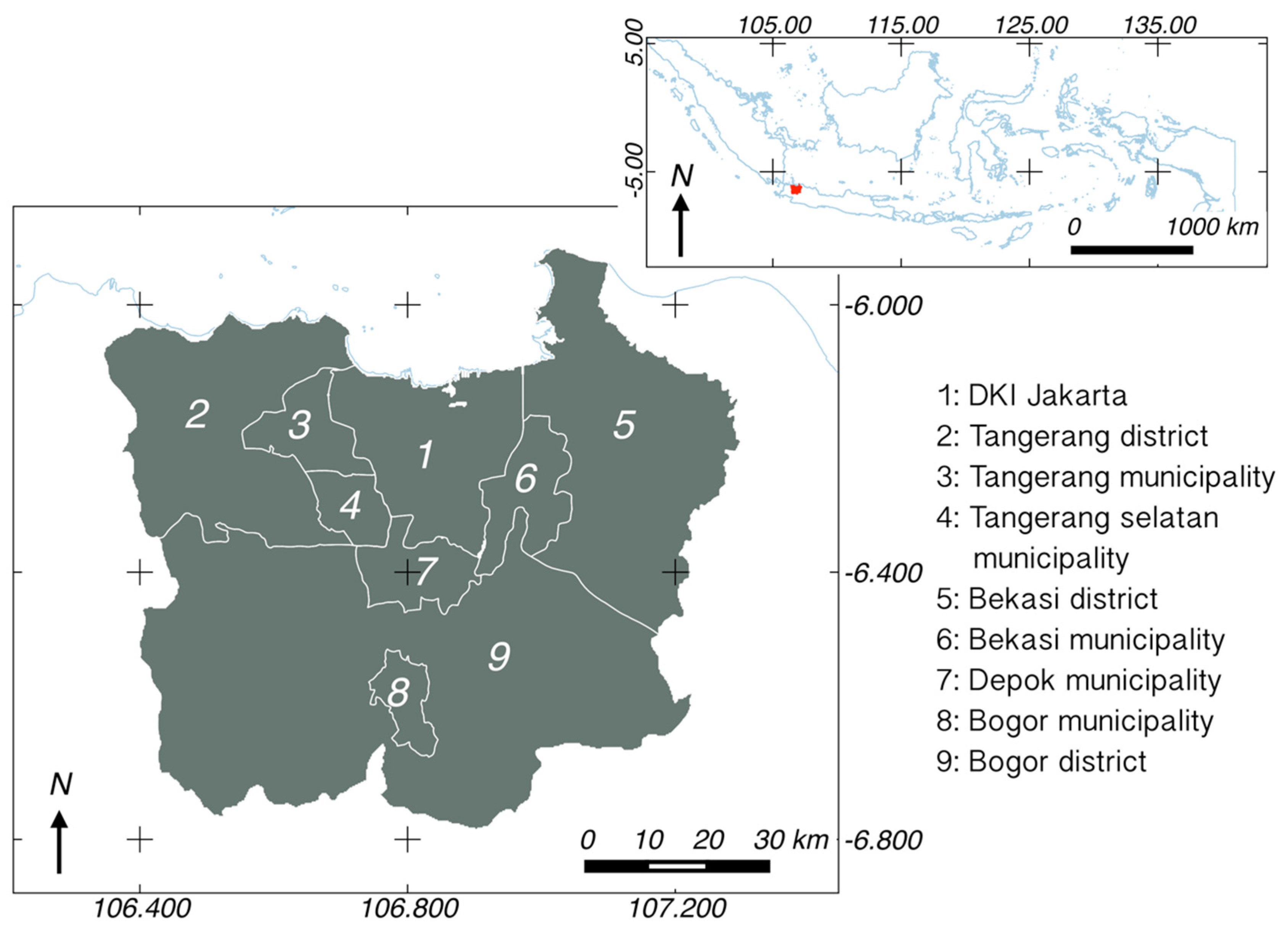
2.1. Study Area
2.2. Data


| 2001 | 2002 | 2003 | 2004 | 2005 | 2006 | 2007 | 2008 | 2009 | 2010 | 2011 | 2012 | 2013 | Total |
|---|---|---|---|---|---|---|---|---|---|---|---|---|---|
| 76 | 120 | 289 | 295 | 235 | 466 | 93 | 123 | 431 | 502 | 325 | 778 | 828 | 4561 |
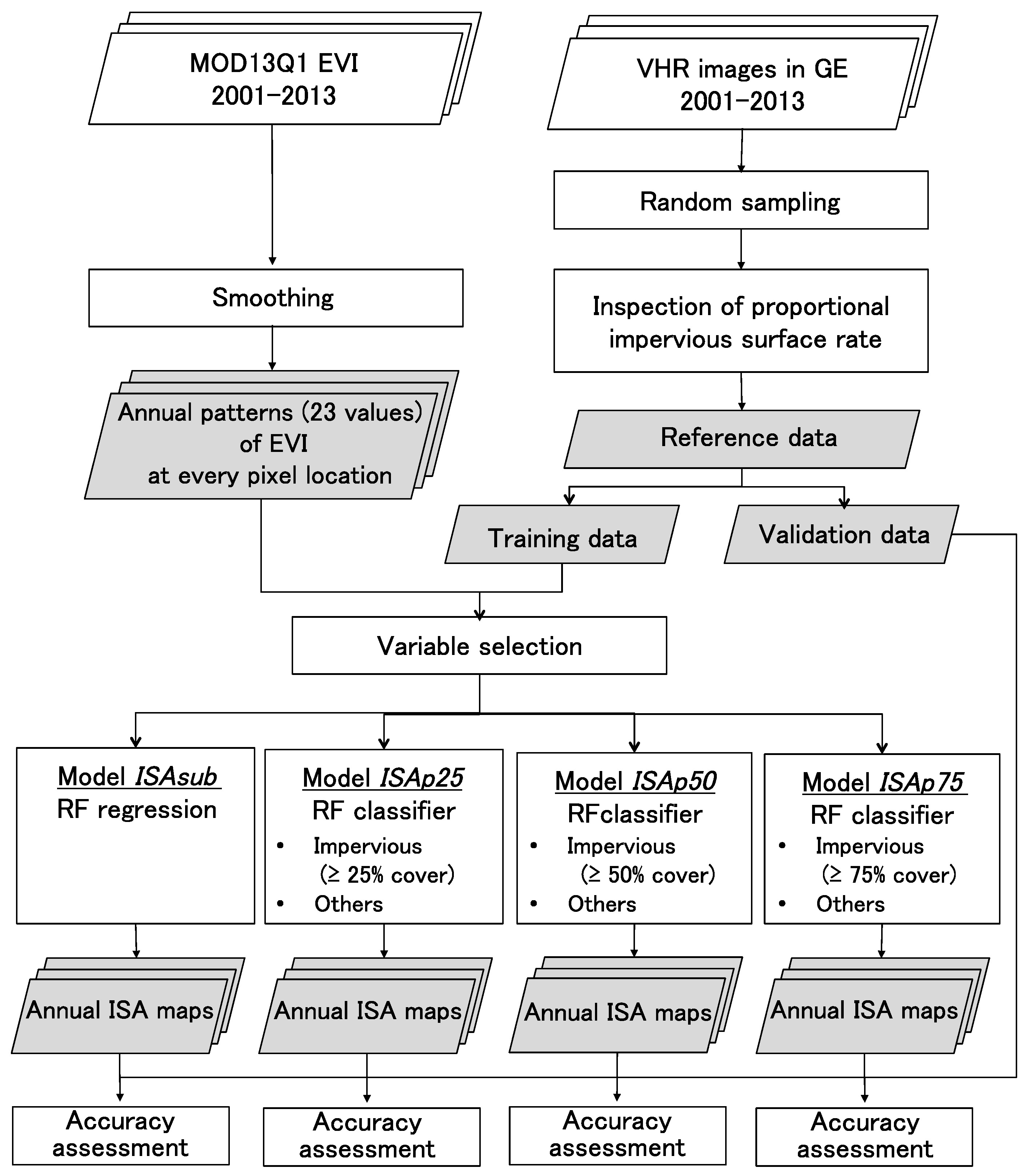
2.3. Analysis
- Model ISAsub: RF regression using ISA proportions as the dependent variable (sub-pixel classification approach)
- Model ISAp25: RF classifier using the Boolean data defined as greater than 25% ISA in the reference pixel (per-pixel classification approach)
- Model ISAp50: RF classifier using the Boolean data defined as greater than 50% ISA in the reference pixel (per-pixel classification approach)
- Model ISAp75: RF classifier using the Boolean data defined as greater than 75% ISA in the reference pixel (per-pixel classification approach)
3. Results
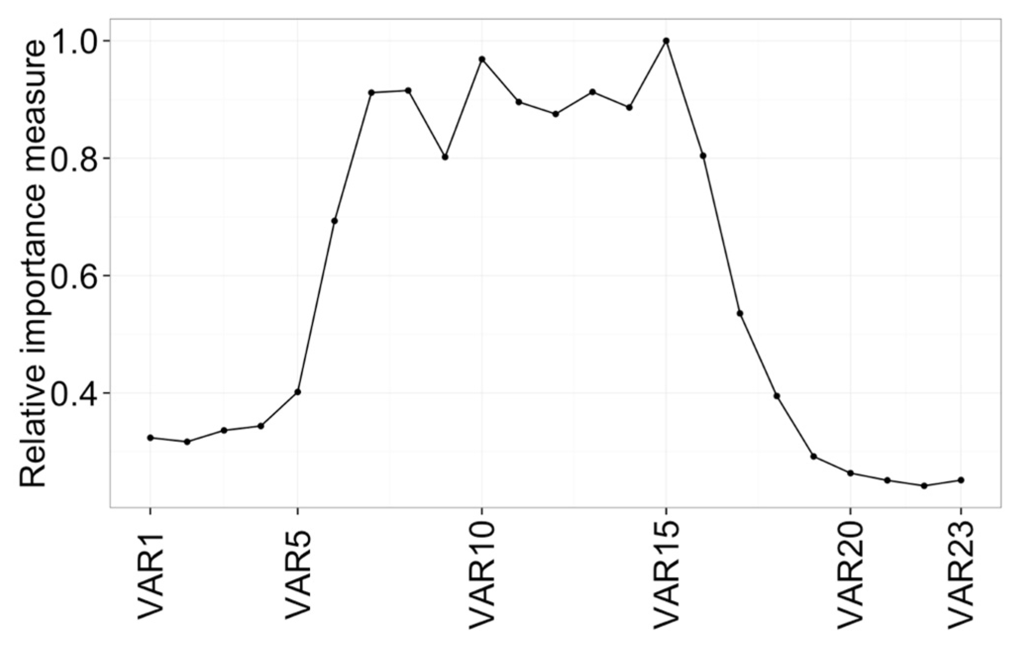
3.1. Model Performance with Different Input Variables
| Selected Variables | Number of Parameters | Variance Explained (%) |
|---|---|---|
| VAR1, 2,…, and 23 | 23 | 58.5 |
| VAR2, 3,…, and 18 | 17 | 58.2 |
| VAR6, 7,…, and 17 | 12 | 56.5 |
| VAR7, 8, 9, 10, 15, and 16 | 6 | 55.3 |
| Model ISAsub (Variance Explained) (%) | Model ISAp25 (OOB Error Rate) (%) | Model ISAp50 (OOB Error Rate) (%) | Model ISAp75 (OOB Error Rate) (%) | |
|---|---|---|---|---|
| 23 variables | 58.5 | 20.7 | 15.1 | 10.8 |
| 4 phenological indices | 52.8 | 24.3 | 16.84 | 11.84 |
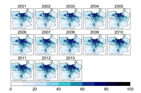
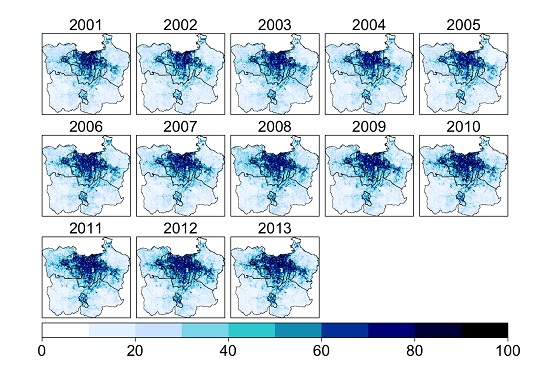
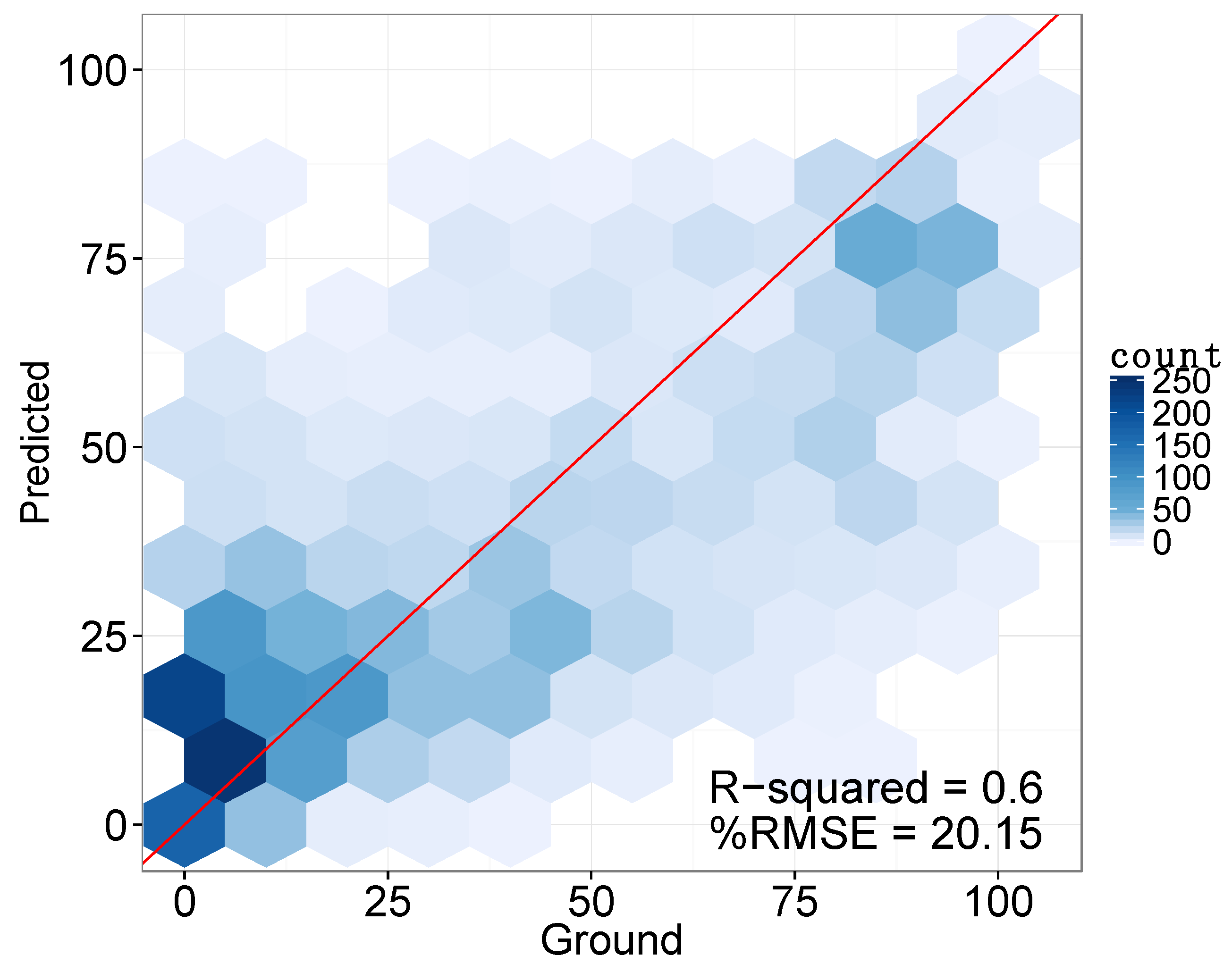
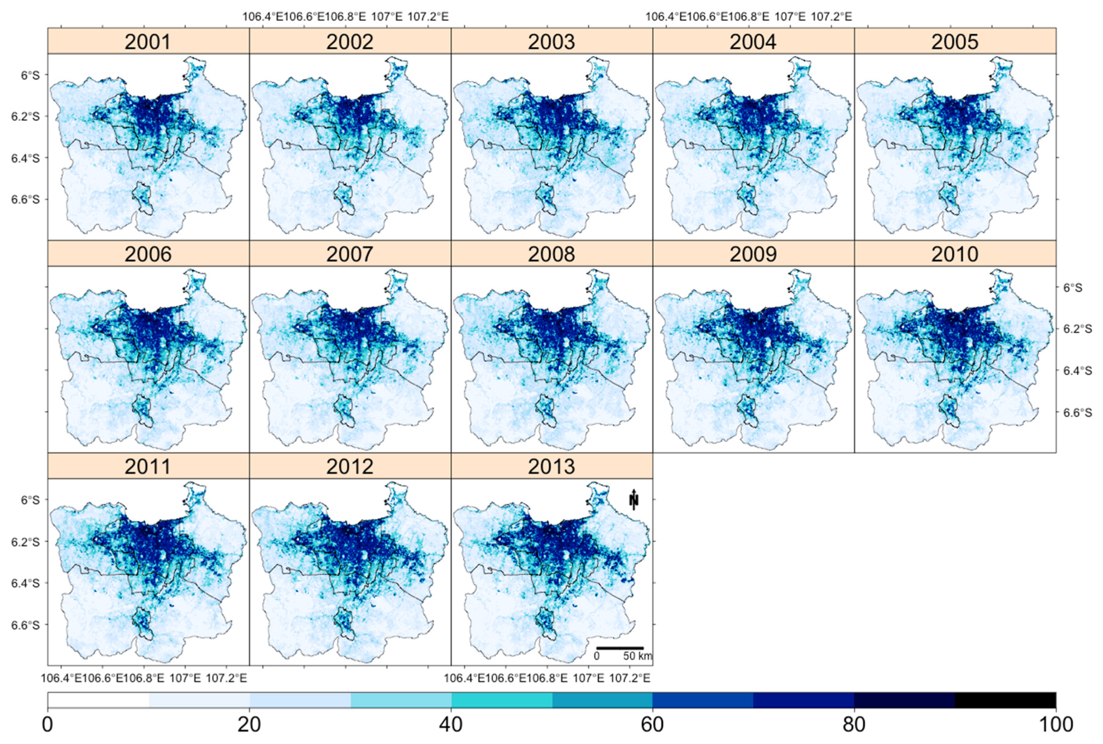
3.2. Sub-Pixel Classification


| 2001 | 2002 | 2003 | 2004 | 2005 | 2006 | 2007 | 2008 | 2009 | 2010 | 2011 | 2012 | 2013 | |
|---|---|---|---|---|---|---|---|---|---|---|---|---|---|
| R-squared | 0.36 | 0.59 | 0.69 | 0.53 | 0.48 | 0.58 | 0.48 | 0.49 | 0.62 | 0.55 | 0.61 | 0.56 | 0.64 |
| %RMSE | 21.75 | 21.01 | 19.39 | 20.35 | 20.74 | 19.67 | 16.39 | 23.88 | 20.05 | 22.07 | 21.59 | 20.18 | 18.05 |
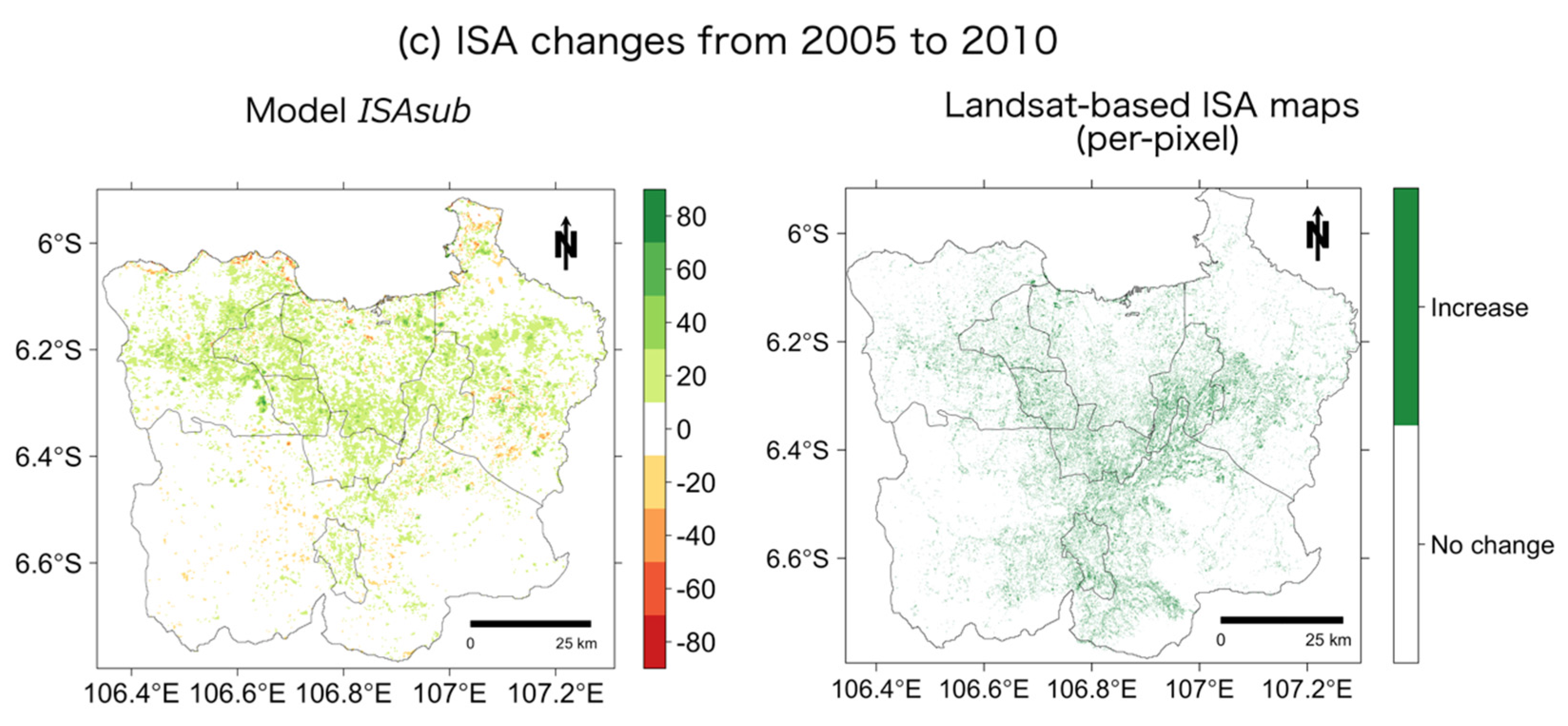
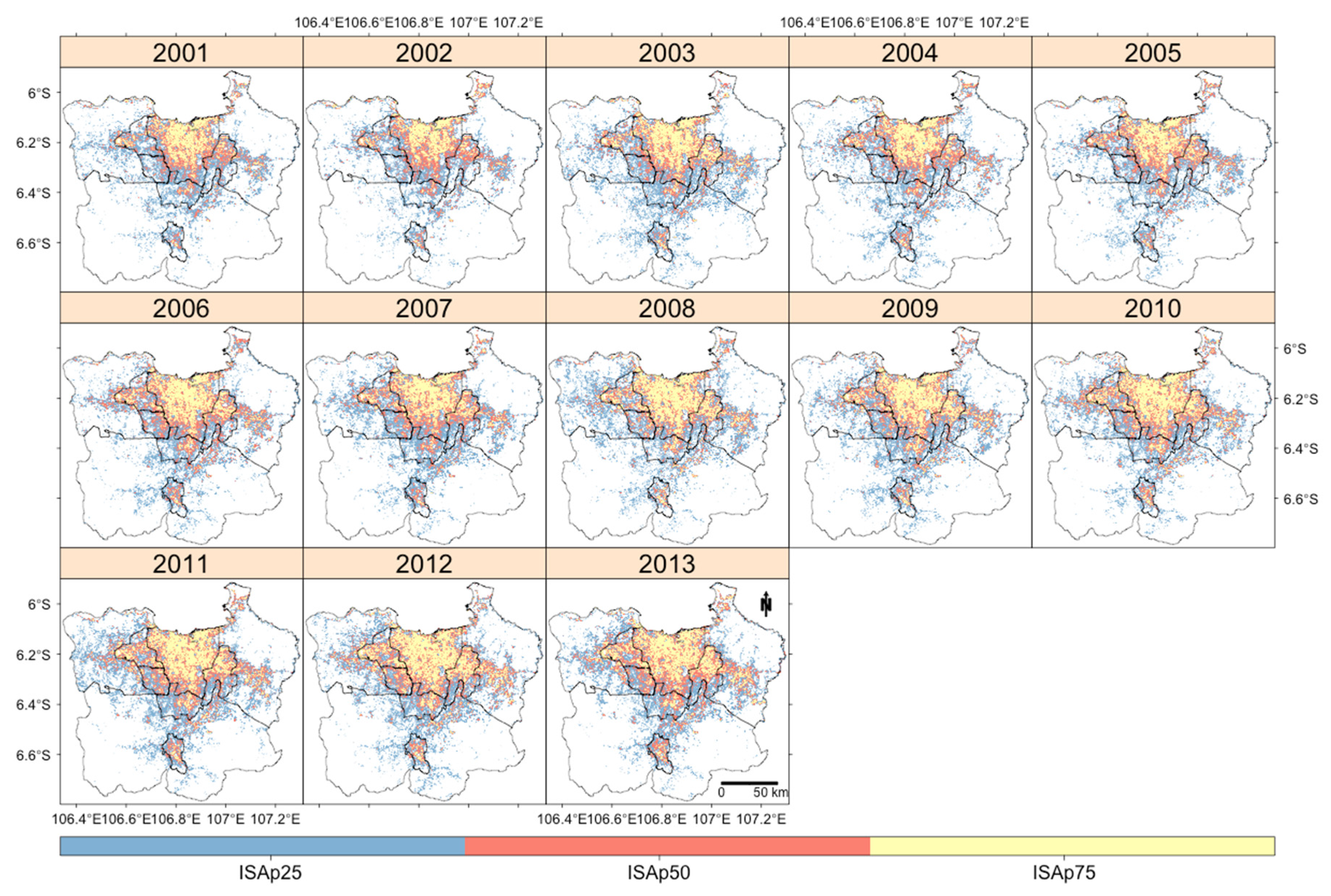
3.3. Per-Pixel Classification
| Model ISAp25 (Overall Accuracy = 0.80) | Model ISAp50 (Overall Accuracy = 0.86) | Model ISAp75 (Overall Accuracy = 0.89) | ||||||||||
|---|---|---|---|---|---|---|---|---|---|---|---|---|
| ISA | Other | Total | User’s | ISA | Other | Total | User’s | ISA | Other | Total | User’s | |
| ISA | 787 | 209 | 996 | 0.79 | 460 | 131 | 591 | 0.78 | 232 | 95 | 327 | 0.71 |
| Other | 241 | 1044 | 1285 | 0.81 | 178 | 1512 | 1690 | 0.90 | 155 | 1799 | 1954 | 0.92 |
| Total | 1028 | 1253 | 2281 | 638 | 1643 | 2281 | 387 | 1894 | 2281 | |||
| Producer’s | 0.77 | 0.83 | 0.72 | 0.92 | 0.60 | 0.95 | ||||||
| Year | Number of Validation data | Overall Accuracy | User’s Accuracy | Producer’s Accuracy | ||||||
|---|---|---|---|---|---|---|---|---|---|---|
| Model ISAp25 | Model ISAp50 | Model ISAp75 | Model ISAp25 | Model ISAp50 | Model ISAp75 | Model ISAp25 | Model ISAp50 | Model ISAp75 | ||
| 2001 | 38 | 0.71 | 0.79 | 0.95 | 0.62 | 0.67 | 0.33 | 0.67 | 0.55 | 1 |
| 2002 | 52 | 0.87 | 0.87 | 0.88 | 0.95 | 0.91 | 1 | 0.75 | 0.62 | 0.4 |
| 2003 | 143 | 0.79 | 0.91 | 0.94 | 0.78 | 0.91 | 0.96 | 0.76 | 0.82 | 0.74 |
| 2004 | 138 | 0.72 | 0.88 | 0.89 | 0.7 | 0.76 | 0.62 | 0.65 | 0.74 | 0.53 |
| 2005 | 126 | 0.78 | 0.83 | 0.9 | 0.8 | 0.68 | 0.67 | 0.62 | 0.45 | 0.15 |
| 2006 | 218 | 0.84 | 0.87 | 0.87 | 0.81 | 0.79 | 0.5 | 0.82 | 0.66 | 0.41 |
| 2007 | 47 | 0.83 | 0.91 | 0.94 | 1 | 0.5 | 0 | 0.43 | 0.25 | 0 |
| 2008 | 67 | 0.76 | 0.79 | 0.84 | 0.78 | 0.79 | 0.83 | 0.88 | 0.73 | 0.65 |
| 2009 | 220 | 0.81 | 0.84 | 0.9 | 0.82 | 0.79 | 0.74 | 0.76 | 0.66 | 0.7 |
| 2010 | 257 | 0.82 | 0.81 | 0.84 | 0.83 | 0.7 | 0.62 | 0.85 | 0.77 | 0.64 |
| 2011 | 146 | 0.84 | 0.84 | 0.82 | 0.86 | 0.87 | 0.77 | 0.90 | 0.81 | 0.62 |
| 2012 | 401 | 0.77 | 0.89 | 0.9 | 0.72 | 0.76 | 0.7 | 0.74 | 0.76 | 0.62 |
| 2013 | 428 | 0.82 | 0.9 | 0.92 | 0.78 | 0.77 | 0.73 | 0.71 | 0.74 | 0.61 |
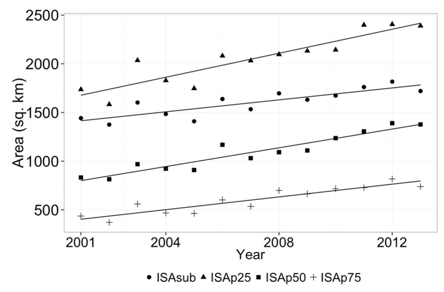
3.4. Estimation of Total ISA
4. Discussion
4.1. Sub-Pixel Classification for Annual Proportional ISA Mappings


4.2. Classification of Annual Patterns of EVI Time Series
4.3. Comparison with Per-Pixel Analyses
4.4. Reference Data
4.5. Future Work
5. Conclusions
Acknowledgments
Author Contributions
Conflicts of Interest
References
- Angel, S.; Parent, J.; Civco, D.L.; Blei, A.; Potere, D. The dimensions of global urban expansion: Estimates and projections for all countries, 2000–2050. Int. J. Remote Sens. 2011, 75, 53–107. [Google Scholar] [CrossRef]
- Weng, Q. Remote sensing of impervious surfaces in the urban areas: Requirements, methods, and trends. Remote Sens. Environ. 2012, 117, 34–49. [Google Scholar] [CrossRef]
- Sexton, J.O.; Song, X.-P.; Huang, C.; Channan, S.; Baker, M.E.; Townshend, J.R. Urban growth of the Washington, D.C.—Baltimore, MD metropolitan region from 1984 to 2010 by annual, Landsat-based estimates of impervious cover. Remote Sens. Environ. 2013, 129, 42–53. [Google Scholar] [CrossRef]
- Arnold, I.C.L.; Gibbons, C.J. Lmpervious suface coverage: The emergence of a key environmental indicator. J. Am. Plan. Assoc. 1996, 62, 243–258. [Google Scholar] [CrossRef]
- Alberti, M. The Effects of Urban Patterns on Ecosystem Function. Int. Reg. Sci. Rev. 2005, 28, 168–192. [Google Scholar] [CrossRef]
- Mcdonald, R.I.; Kareiva, P.; Forman, R.T.T. The implications of current and future urbanization for global protected areas and biodiversity conservation. Biol. Conserv. 2008, 141, 1695–1703. [Google Scholar] [CrossRef]
- Rojas, C.; Pino, J.; Basnou, C.; Vivanco, M. Assessing land-use and -cover changes in relation to geographic factors and urban planning in the metropolitan area of Concepción (Chile). Implications for biodiversity conservation. Appl. Geogr. 2013, 39, 93–103. [Google Scholar] [CrossRef]
- Yang, L.; Xian, G.; Klaver, J.M.; Deal, B. Urban land-cover change detection through sub-pixel imperviousness mapping using remotely sensed data. Photogramm. Eng. Remote Sens. 2003, 69, 1003–1010. [Google Scholar] [CrossRef]
- Schneider, A.; Friedl, M.A.; Potere, D. A new map of global urban extent from MODIS satellite data. Environ. Res. Lett. 2009, 4, 044003. [Google Scholar] [CrossRef]
- Knight, J.; Voth, M. Mapping impervious cover using multi-temporal MODIS NDVI data. IEEE J. Sel. Top. Appl. Earth Obs. Remote Sens. 2011, 4, 303–309. [Google Scholar] [CrossRef]
- Tsutsumida, N.; Saizen, I.; Matsuoka, M.; Ishii, R. Land cover change detection in Ulaanbaatar using the breaks for additive seasonal and trend method. Land 2013, 2, 534–549. [Google Scholar] [CrossRef]
- Lunetta, R.S.; Knight, J.F.; Ediriwickrema, J.; Lyon, J.G.; Worthy, L.D. Land-cover change detection using multi-temporal MODIS NDVI data. Remote Sens. Environ. 2006, 105, 142–154. [Google Scholar] [CrossRef]
- Clark, M.L.; Aide, T.M.; Riner, G. Land change for all municipalities in Latin America and the Caribbean assessed from 250-m MODIS imagery (2001–2010). Remote Sens. Environ. 2012, 126, 84–103. [Google Scholar] [CrossRef]
- Clark, M.L.; Aide, T.M.; Grau, H.R.; Riner, G. A scalable approach to mapping annual land cover at 250 m using MODIS time series data: A case study in the Dry Chaco ecoregion of South America. Remote Sens. Environ. 2010, 114, 2816–2832. [Google Scholar] [CrossRef]
- Sánchez-Cuervo, A.M.; Aide, T.M.; Clark, M.L.; Etter, A. Land cover change in Colombia: Surprising forest recovery trends between 2001 and 2010. PLoS ONE 2012, 7, e43943. [Google Scholar] [CrossRef] [PubMed]
- Álvarez-berríos, N.L.; Redo, D.J.; Aide, T.M.; Clark, M.L.; Grau, R. Land change in the Greater Antilles between 2001 and 2010. Land 2013, 2, 81–107. [Google Scholar] [CrossRef]
- Fisher, P. The pixel: A snare and a delusion. Int. J. Remote Sens. 1997, 18, 679–685. [Google Scholar] [CrossRef]
- Foody, G.M.; Arora, M.K. Incorporating mixed pixels in the training, allocation and testing stages of supervised classifications. Pattern Recognit. Lett. 1996, 17, 1389–1398. [Google Scholar] [CrossRef]
- Arnot, C.; Fisher, P.F.; Wadsworth, R.; Wellens, J. Landscape metrics with ecotones: Pattern under uncertainty. Landsc. Ecol. 2004, 19, 181–195. [Google Scholar] [CrossRef]
- Shao, Y.; Lunetta, R.S. Sub-pixel mapping of tree canopy, impervious surfaces, and cropland in the Laurentian Great Lakes Basin using MODIS time-series data. IEEE J. Sel. Top. Appl. Earth Obs. Remote Sens. 2011, 4, 336–347. [Google Scholar] [CrossRef]
- Colditz, R.R.; López Saldaña, G.; Maeda, P.; Espinoza, J.A.; Tovar, C.M.; Hernández, A.V.; Benítez, C.Z.; Cruz López, I.; Ressl, R. Generation and analysis of the 2005 land cover map for Mexico using 250m MODIS data. Remote Sens. Environ. 2012, 123, 541–552. [Google Scholar] [CrossRef]
- Foody, G.M. Status of land cover classification accuracy assessment. Remote Sens. Environ. 2002, 80, 185–201. [Google Scholar] [CrossRef]
- Li, M. A review of remote sensing image classification techniques: The role of spatio-contextual information. Eur. J. Remote Sens. 2014, 47, 389–411. [Google Scholar] [CrossRef]
- Xu, M.; Watanachaturaporn, P.; Varshney, P.; Arora, M. Decision tree regression for soft classification of remote sensing data. Remote Sens. Environ. 2005, 97, 322–336. [Google Scholar] [CrossRef]
- Zhang, J.; Foody, G.M. Fully-fuzzy supervised classification of sub-urban land cover from remotely sensed imagery: Statistical and artificial neural network approaches. Int. J. Remote Sens. 2001, 22, 615–628. [Google Scholar] [CrossRef]
- Zhang, J.; Foody, G.M. A fuzzy classification of sub-urban land cover from remotely sensed imagery. Int. J. Remote Sens. 1998, 19, 2721–2738. [Google Scholar] [CrossRef]
- Yang, F.; Matsushita, B.; Yang, W.; Fukushima, T. Mapping the human footprint from satellite measurements in Japan. ISPRS J. Photogramm. Remote Sens. 2014, 88, 80–90. [Google Scholar] [CrossRef] [Green Version]
- Lu, D.; Moran, E.; Hetrick, S. Detection of impervious surface change with multitemporal Landsat images in an urban-rural frontier. ISPRS J. Photogramm. Remote Sens. 2011, 66, 298–306. [Google Scholar] [CrossRef] [PubMed]
- Wu, C.; Murray, A.T. Estimating impervious surface distribution by spectral mixture analysis. Remote Sens. Environ. 2003, 84, 493–505. [Google Scholar] [CrossRef]
- Yuan, F.; Bauer, M.E. Comparison of impervious surface area and normalized difference vegetation index as indicators of surface urban heat island effects in Landsat imagery. Remote Sens. Environ. 2007, 106, 375–386. [Google Scholar] [CrossRef]
- Deng, C.; Wu, C. The use of single-date MODIS imagery for estimating large-scale urban impervious surface fraction with spectral mixture analysis and machine learning techniques. ISPRS J. Photogramm. Remote Sens. 2013, 86, 100–110. [Google Scholar] [CrossRef]
- Rogan, J.; Franklin, J.; Stow, D.; Miller, J.; Woodcock, C.; Roberts, D. Mapping land-cover modifications over large areas: A comparison of machine learning algorithms. Remote Sens. Environ. 2008, 112, 2272–2283. [Google Scholar] [CrossRef]
- Strahler, A.H.; Boschetti, L.; Foody, G.M.; Friedl, M.A.; Hansen, M.C.; Herold, M.; Mayaux, P.; Morisette, J.T.; Stehman, S.V.; Woodcock, C.E. Global Land Cover Validation: Recommendations for Evaluation and Accuracy Assessment of Global Land Cover Maps. Available online: https://core.ac.uk/display/20728200 (accessed on 14 February 2016).
- Chen, J.; Zhu, X.; Imura, H.; Chen, X. Consistency of accuracy assessment indices for soft classification: Simulation analysis. ISPRS J. Photogramm. Remote Sens. 2010, 65, 156–164. [Google Scholar] [CrossRef]
- Lu, D.; Moran, E.; Batistella, M. Linear mixture model applied to Amazonian vegetation classification. Remote Sens. Environ. 2003, 87, 456–469. [Google Scholar] [CrossRef] [Green Version]
- Adams, J. Classification of multispectral images based on fractions of endmembers: Application to land-cover change in the Brazilian Amazon. Remote Sens. Environ. 1995, 52, 137–154. [Google Scholar] [CrossRef]
- Walton, J.T. Subpixel urban land cover estimation: comparing cubist, random forests, and support vector regression. Photogramm. Eng. Remote Sens. 2008, 74, 1213–1222. [Google Scholar] [CrossRef]
- Esch, T.; Himmler, V.; Schorcht, G.; Thiel, M.; Wehrmann, T.; Bachofer, F.; Conrad, C.; Schmidt, M.; Dech, S. Large-area assessment of impervious surface based on integrated analysis of single-date Landsat-7 images and geospatial vector data. Remote Sens. Environ. 2009, 113, 1678–1690. [Google Scholar] [CrossRef]
- Yuan, F.; Wu, C.; Bauer, M.E. Comparison of spectral analysis techniques for impervious surface estimation using landsat imagery. Photogramm. Eng. Remote Sens. 2008, 74, 1045–1055. [Google Scholar] [CrossRef]
- Gislason, P.O.; Benediktsson, J.A.; Sveinsson, J.R. Random Forests for land cover classification. Pattern Recognit. Lett. 2006, 27, 294–300. [Google Scholar] [CrossRef]
- Pal, M. Random forest classifier for remote sensing classification. Int. J. Remote Sens. 2005, 26, 217–222. [Google Scholar] [CrossRef]
- Rodriguez-Galiano, V.F.; Chica-Olmo, M.; Abarca-Hernandez, F.; Atkinson, P.M.; Jeganathan, C. Random Forest classification of Mediterranean land cover using multi-seasonal imagery and multi-seasonal texture. Remote Sens. Environ. 2012, 121, 93–107. [Google Scholar] [CrossRef]
- Wang, J.; Zhao, Y.; Li, C.; Yu, L.; Liu, D.; Gong, P. Mapping global land cover in 2001 and 2010 with spatial-temporal consistency at 250 m resolution. ISPRS J. Photogramm. Remote Sens. 2015, 103, 38–47. [Google Scholar] [CrossRef]
- Balzter, H.; Cole, B.; Thiel, C.; Schmullius, C. Mapping CORINE land cover from Sentinel-1A SAR and SRTM digital elevation model data using Random Forests. Remote Sens. 2015, 7, 14876–14898. [Google Scholar] [CrossRef]
- Reschke, J.; Hüttich, C. Continuous field mapping of Mediterranean wetlands using sub-pixel spectral signatures and multi-temporal Landsat data. Int. J. Appl. Earth Obs. Geoinf. 2014, 28, 220–229. [Google Scholar] [CrossRef]
- Pravitasari, A.E.; Saizen, I.; Tsutsumida, N.; Rustiadi, E.; Pribadi, D.O. Local spatially dependent driving forces of urban expansion in an emerging Asian Megacity: The case of Greater Jakarta (Jabodetabek). J. Sustain. Dev. 2015, 8, 108–119. [Google Scholar] [CrossRef]
- Hudalah, D.; Firman, T. Beyond property: Industrial estates and post-suburban transformation in Jakarta Metropolitan Region. Cities 2012, 29, 40–48. [Google Scholar] [CrossRef]
- Pravitasari, A.E.; Saizen, I.; Tsutsumida, N.; Rustiadi, E. Detection of spatial clusters of flood- and landslide-prone areas using local moran index in Jabodetabek Metropolitan Area, Indonesia. Int. J. Ecol. Environ. Sci. 2014, 40, 223–243. [Google Scholar]
- Schneider, A.; Mertes, C.M.; Tatem, A.J.; Tan, B.; Sulla-Menashe, D.; Graves, S.J.; Patel, N.N.; Horton, J.A.; Gaughan, A.E.; Rollo, J.T.; et al. A new urban landscape in East-Southeast Asia, 2000–2010. Environ. Res. Lett. 2015, 10, 034002. [Google Scholar] [CrossRef]
- Rustiadi, E.; Iman, L.O.S.; Lufitayanti, T.; Pravitasari, A.E. LUCC inconsistency analysis to spatial plan and land capability (case study: Jabodetabek region). In SLUAS Science Report 2013; Himiyama, Y., Ed.; Toward Sustainable Landuse in Asia (IV); Institute of Geography, Hokkaido University of Education: Asahikawa, Japan, 2013; pp. 123–131. [Google Scholar]
- Huete, A.; Didan, K.; Miura, T.; Rodriguez, E.; Gao, X.; Ferreira, L. Overview of the radiometric and biophysical performance of the MODIS vegetation indices. Remote Sens. Environ. 2002, 83, 195–213. [Google Scholar] [CrossRef]
- Schneider, A.; Friedl, M.A.; Potere, D. Mapping global urban areas using MODIS 500-m data: New methods and datasets based on “urban ecoregions”. Remote Sens. Environ. 2010, 114, 1733–1746. [Google Scholar] [CrossRef]
- Jönsson, P.; Eklundh, L. TIMESAT—A program for analyzing time-series of satellite sensor data. Comput. Geosci. 2004, 30, 833–845. [Google Scholar] [CrossRef]
- Eklundh, L.; Jönsson, P. TIMESAT 3.1 Software Manual; Lund University: Lund, Sweden, 2012. [Google Scholar]
- Tsutsumida, N.; Comber, A.J. Measures of spatio-temporal accuracy for time series land cover data. Int. J. Appl. Earth Obs. Geoinf. 2015, 41, 46–55. [Google Scholar] [CrossRef]
- Kobayashi, T.; Tsend-Ayush, J.; Tateishi, R. A new tree cover percentage map in Eurasia at 500 m resolution using MODIS data. Remote Sens. 2014, 6, 209–232. [Google Scholar] [CrossRef]
- Kontgis, C.; Schneider, A.; Fox, J.; Saksena, S.; Spencer, J.H.; Castrence, M. Monitoring peri-urbanization in the greater Ho Chi Minh City metropolitan area. Appl. Geogr. 2014, 53, 377–388. [Google Scholar] [CrossRef]
- Schneider, A. Monitoring land cover change in urban and peri-urban areas using dense time stacks of Landsat satellite data and a data mining approach. Remote Sens. Environ. 2012, 124, 689–704. [Google Scholar] [CrossRef]
- Breiman, L. Random forests. Mach. Learn. 2001, 45, 5–32. [Google Scholar] [CrossRef]
- Liaw, A.; Wiener, M. Classification and regression by randomForest. R. News 2002, 2, 18–22. [Google Scholar]
- Senf, C.; Hostert, P.; Linden, S.; Van Der Berlin, H.; Linden, U. Den Using MODIS time series and random forest classification for mapping land use in South-East Asia. In Proceedings of the IEEE International Geoscience and Remote Sensing Symposium (IGARSS), Munich, Germany, 22–27 July 2012; pp. 6733–6736.
- Evans, J.S.; Murphy, M.A. rfUtilities. R Package Version 1.0–0. Available online: http://CRAN.R-project.org/package=rfUtilities (accessed on 4 February 2016).
- Murphy, M.A.; Evans, J.S.; Storfer, A. Quantifying Bufo boreas connectivity in Yellowstone National Park with landscape genetics. Ecology 2010, 91, 252–261. [Google Scholar] [CrossRef] [PubMed]
- Rodriguez-Galiano, V.F.; Ghimire, B.; Rogan, J.; Chica-Olmo, M.; Rigol-Sanchez, J.P. An assessment of the effectiveness of a Random Forest classifier for land-cover classification. ISPRS J. Photogramm. Remote Sens. 2012, 67, 93–104. [Google Scholar] [CrossRef]
- Mitchell, M.W. Bias of the Random Forest Out-of-Bag (OOB) error for certain input Parameters. Open J. Stat. 2011, 1, 205–211. [Google Scholar] [CrossRef]
- Stehman, S.V.; Czaplewski, R.L. Design and analysis for Thematic Map Accuracy Assessment. Remote Sens. Environ. 1998, 64, 331–344. [Google Scholar] [CrossRef]
- Hansen, M.C.; Loveland, T.R. A review of large area monitoring of land cover change using Landsat data. Remote Sens. Environ. 2012, 122, 66–74. [Google Scholar] [CrossRef]
- Rustiadi, E.; Pribadi, D.O.; Pravitasari, A.E.; Agrisantika, T. The Dynamics of Population, Economic Hegemony and Land Use/Cover Change of Jabodetabek Region (Jakarta Megacity). In Land Use/Cover Changes in Selected Regions in the World; Himiyama, Y., Bičik, I., Eds.; International Geographical Union Commission on Land Use and Land Cover Change: Asahikawa, Japan, 2012; Volume IV, pp. 51–56. [Google Scholar]
- Tewkesbury, A.P.; Comber, A.J.; Tate, N.J.; Lamb, A.; Fisher, P.F. A critical synthesis of remotely sensed optical image change detection techniques. Remote Sens. Environ. 2015, 160, 1–14. [Google Scholar] [CrossRef]
- Farah, A.; Algarni, D. Positional accuracy assessment of Googleearth in Riyadh. Artif. Satell. 2014, 49, 8–13. [Google Scholar] [CrossRef]
- Mohammed, N.Z.; Ghazi, A.; Mustafa, H.E. Positional accuracy testing of Google Earth. Int. J. Multidiscip. Sci. Eng. 2013, 4, 6–9. [Google Scholar]
- Paredes-Hernández, C.U.; Salinas-Castillo, W.E.; Guevara-Cortina, F.; Martínez-Becerra, X. Horizontal positional accuracy of Google Earth’s imagery over rural areas: A study case in Tamaulipas, Mexico. Bol. Ciencias Geod. 2013, 19, 588–601. [Google Scholar] [CrossRef]
- Permissions—Google: Using Google Maps, Google Earth and Street View. Available online: https://www.google.com/permissions/geoguidelines.html#streetview (accessed on 28 December 2015).
- Colditz, R. An evaluation of different training sample allocation schemes for discrete and continuous land cover classification using decision tree-based algorithms. Remote Sens. 2015, 7, 9655–9681. [Google Scholar] [CrossRef]
- Foody, G.M. Assessing the accuracy of land cover change with imperfect ground reference data. Remote Sens. Environ. 2010, 114, 2271–2285. [Google Scholar] [CrossRef]
- Comber, A.; Fisher, P.; Wadsworth, R. What is land cover? Environ. Plan. B Plan. Des. 2005, 32, 199–209. [Google Scholar] [CrossRef]
- Comber, A.J.; Fisher, P.; Brunsdon, C.; Khmag, A. Spatial analysis of remote sensing image classification accuracy. Remote Sens. Environ. 2012, 127, 237–246. [Google Scholar] [CrossRef]
- Foody, G.M. Local characterization of thematic classification accuracy through spatially constrained confusion matrices. Int. J. Remote Sens. 2005, 26, 1217–1228. [Google Scholar] [CrossRef]
- Comber, A.J. Geographically weighted methods for estimating local surfaces of overall, user and producer accuracies. Remote Sens. Lett. 2013, 4, 373–380. [Google Scholar] [CrossRef]
- Kirmanto, D.; Ernawi, I.S.; Djakapermana, R.D. Indonesia green city development program: An urban reform. In Proceedings of the 48th ISOCARP Congress 2012, Perm, Russia, 10–13 September 2012; pp. 1–13.
© 2016 by the authors; licensee MDPI, Basel, Switzerland. This article is an open access article distributed under the terms and conditions of the Creative Commons by Attribution (CC-BY) license (http://creativecommons.org/licenses/by/4.0/).
Share and Cite
Tsutsumida, N.; Comber, A.; Barrett, K.; Saizen, I.; Rustiadi, E. Sub-Pixel Classification of MODIS EVI for Annual Mappings of Impervious Surface Areas. Remote Sens. 2016, 8, 143. https://doi.org/10.3390/rs8020143
Tsutsumida N, Comber A, Barrett K, Saizen I, Rustiadi E. Sub-Pixel Classification of MODIS EVI for Annual Mappings of Impervious Surface Areas. Remote Sensing. 2016; 8(2):143. https://doi.org/10.3390/rs8020143
Chicago/Turabian StyleTsutsumida, Narumasa, Alexis Comber, Kirsten Barrett, Izuru Saizen, and Ernan Rustiadi. 2016. "Sub-Pixel Classification of MODIS EVI for Annual Mappings of Impervious Surface Areas" Remote Sensing 8, no. 2: 143. https://doi.org/10.3390/rs8020143