
Ground-Based Hyperspectral Image Analysis of the Lower Mississippian (Osagean) Reeds Spring Formation Rocks in Southwestern Missouri

Abstract
:
1. Introduction
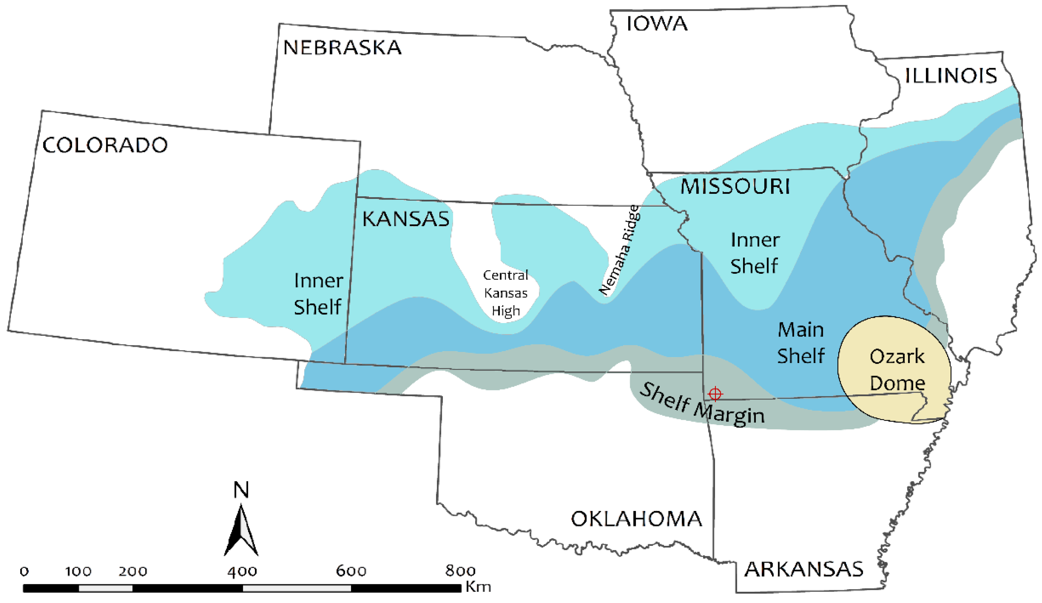
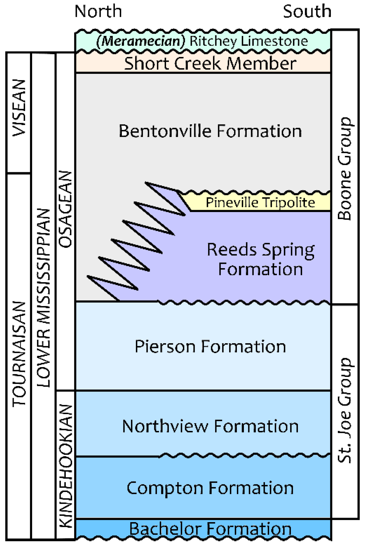
1.1. Geological Setting
1.2. Overview of Tripolite
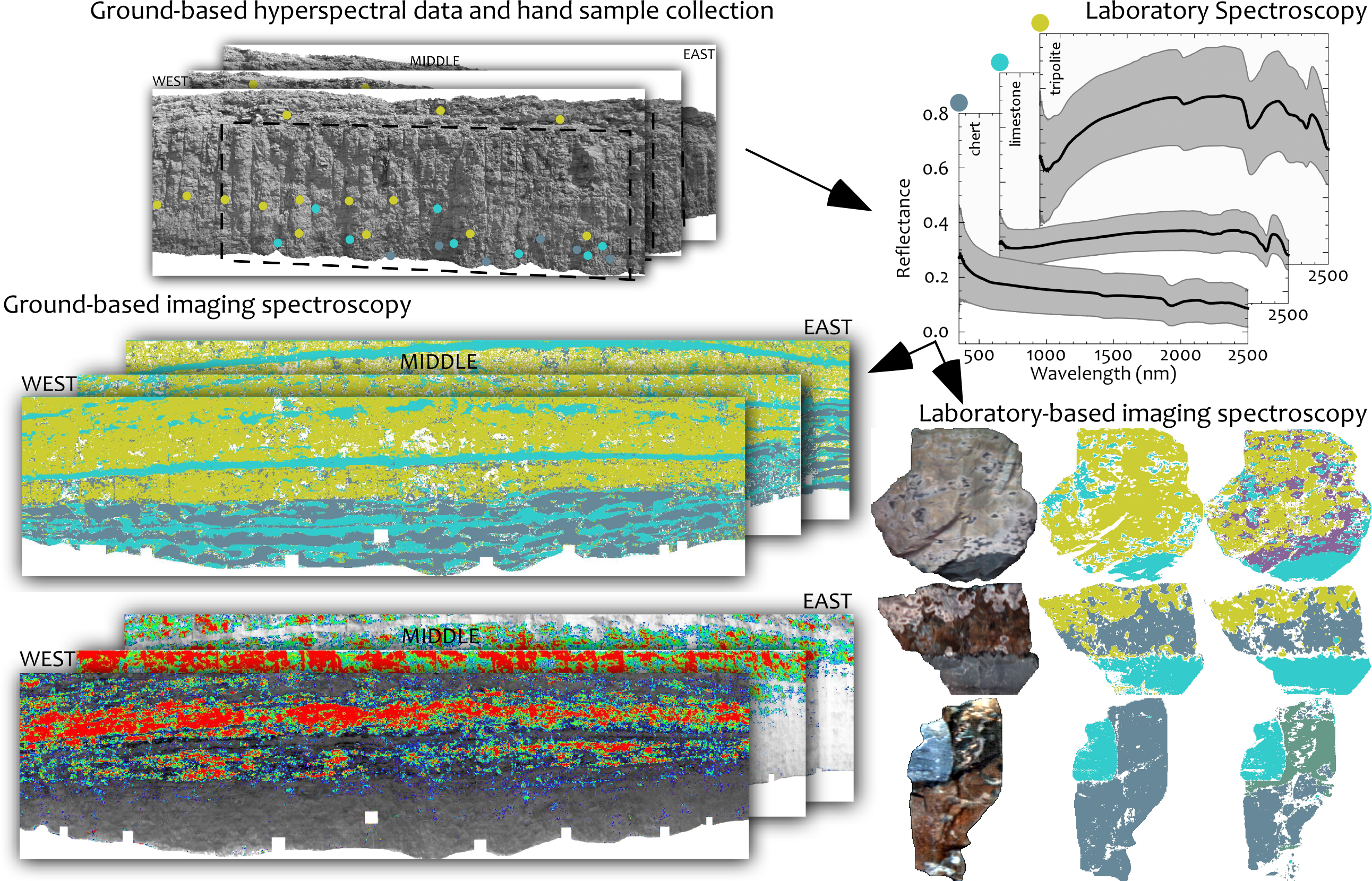
2. Materials and Methods
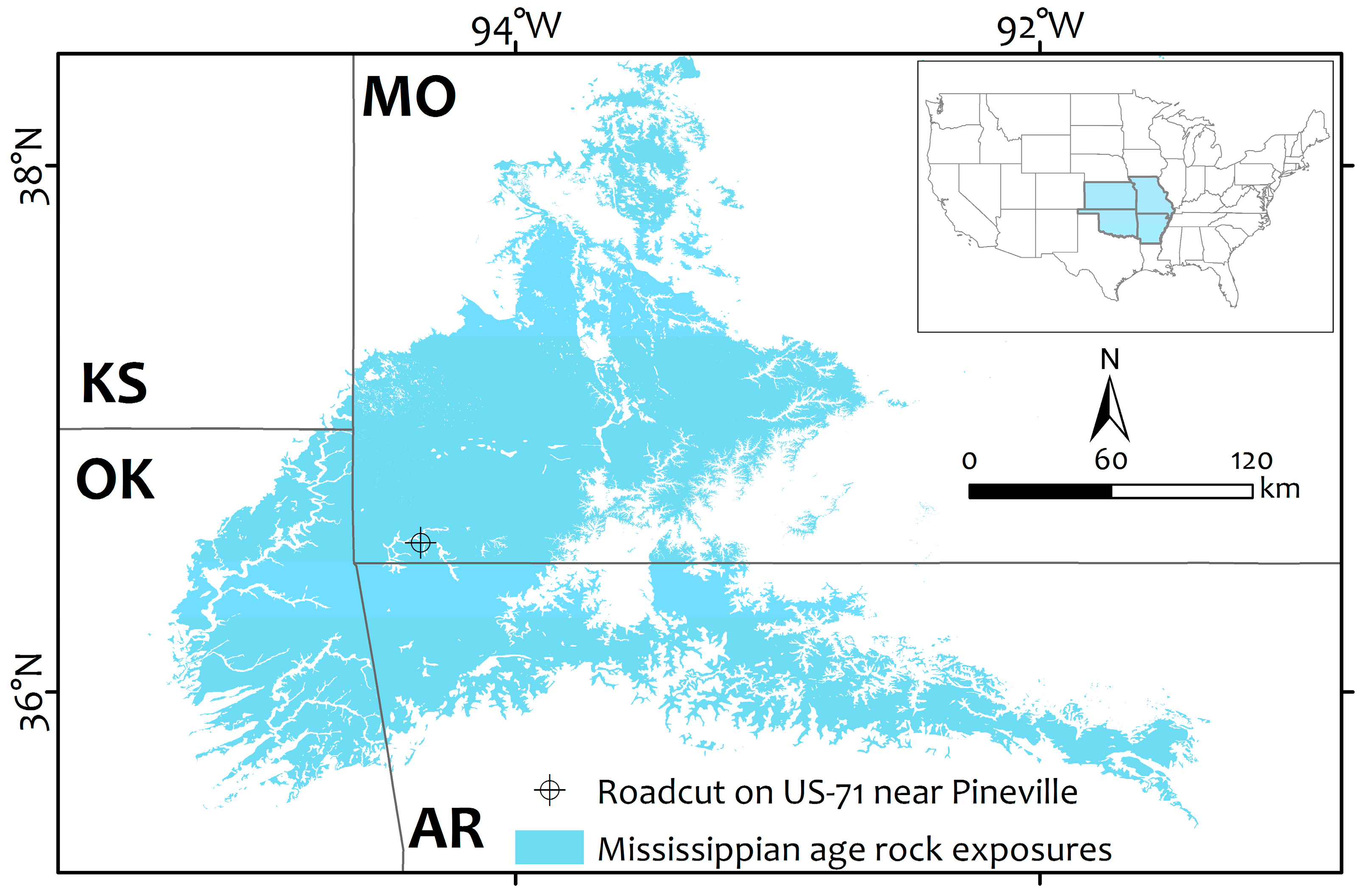
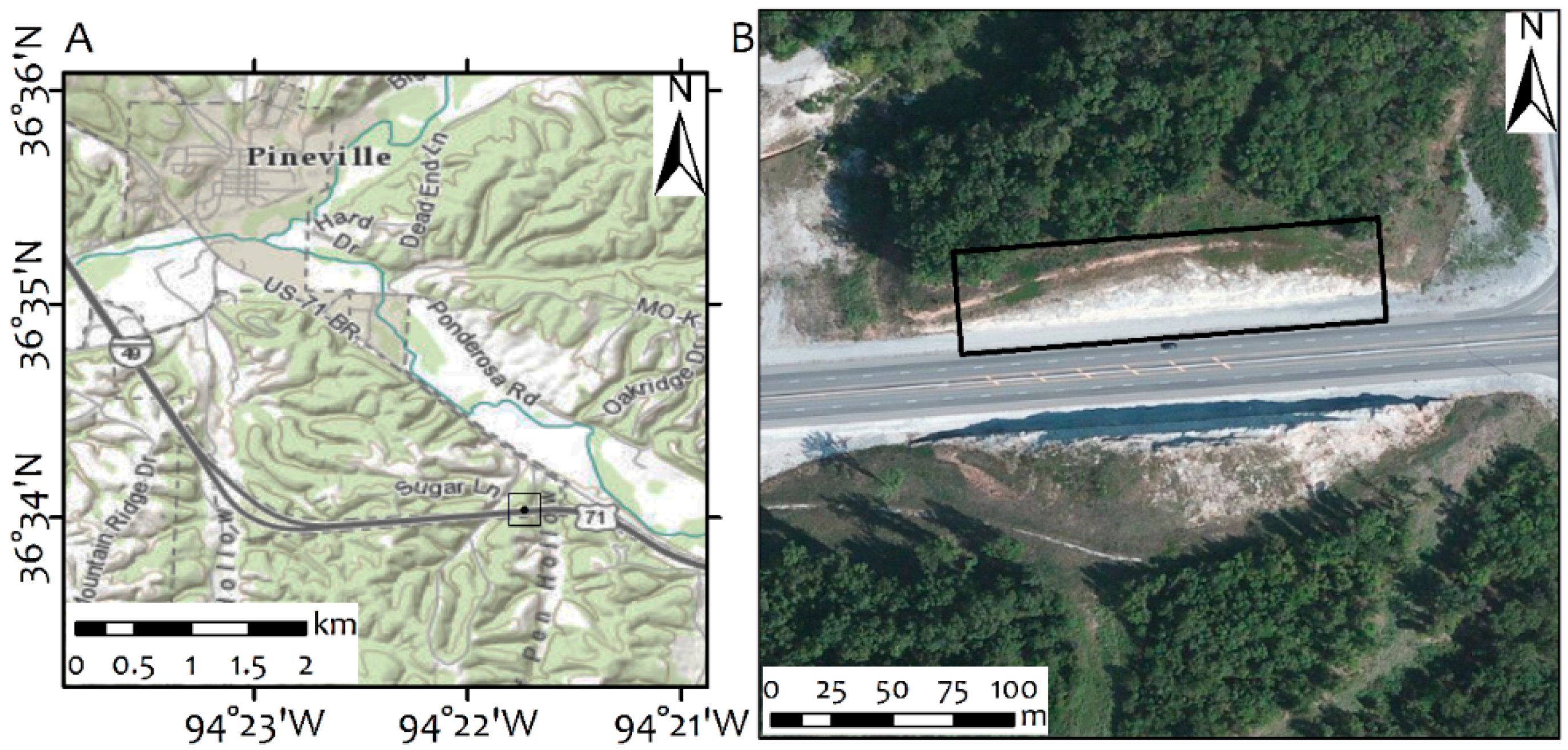
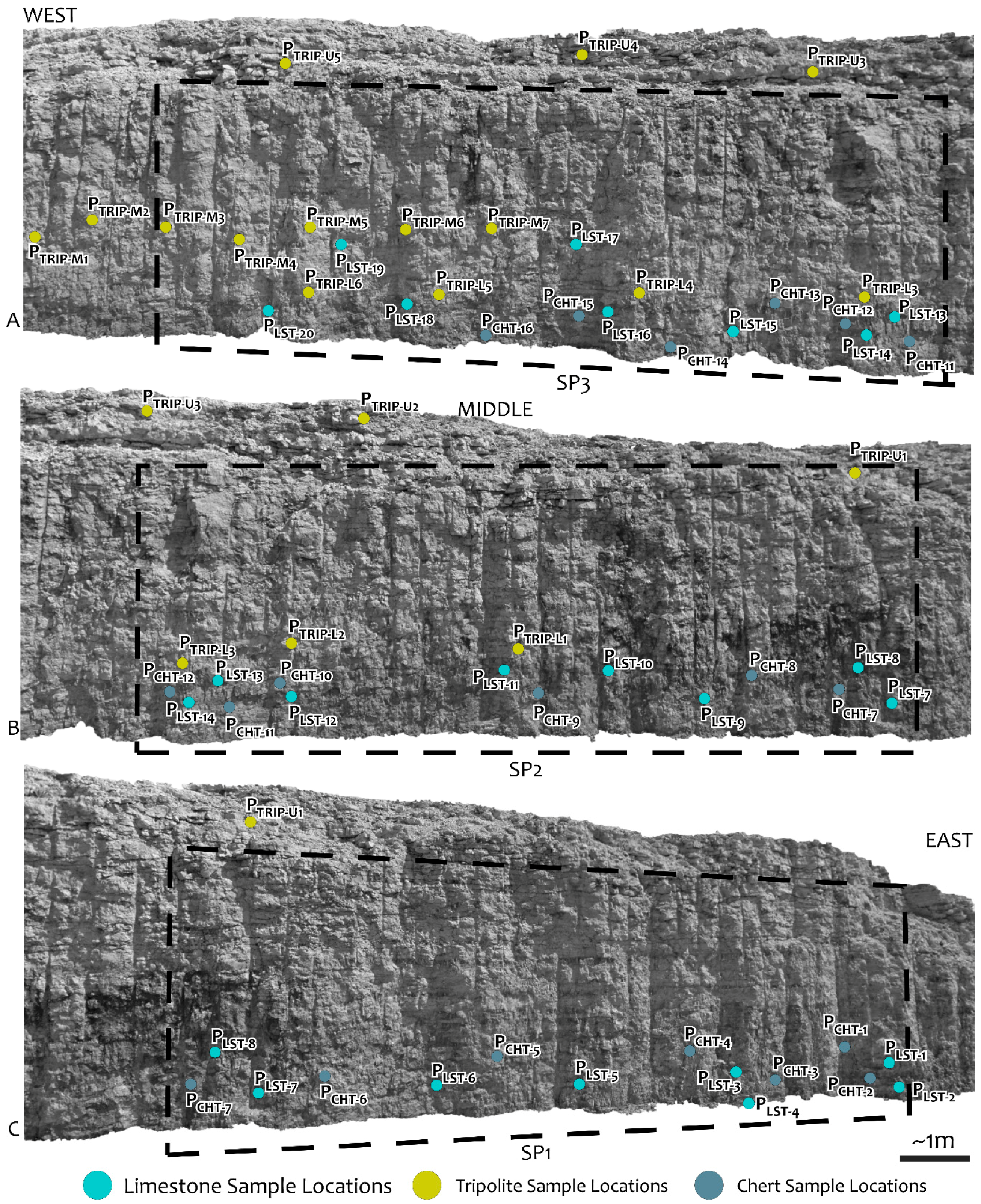
2.1. Study Area
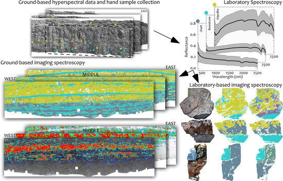
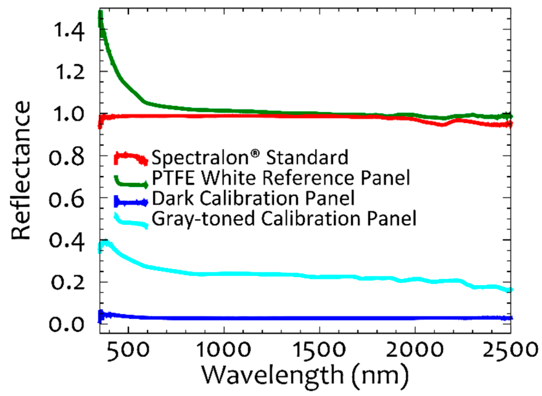
2.2. Instrumentation and Data Collection
2.3. Laboratory Reflectance Spectroscopy
2.4. Ground- and Laboratory-Based Hyperspectral Image Pre-Processing
2.5. Spectral Mapping
2.5.1. Spectral End-Member Extraction
2.5.2. Hyperspectral Image Classification
3. Results
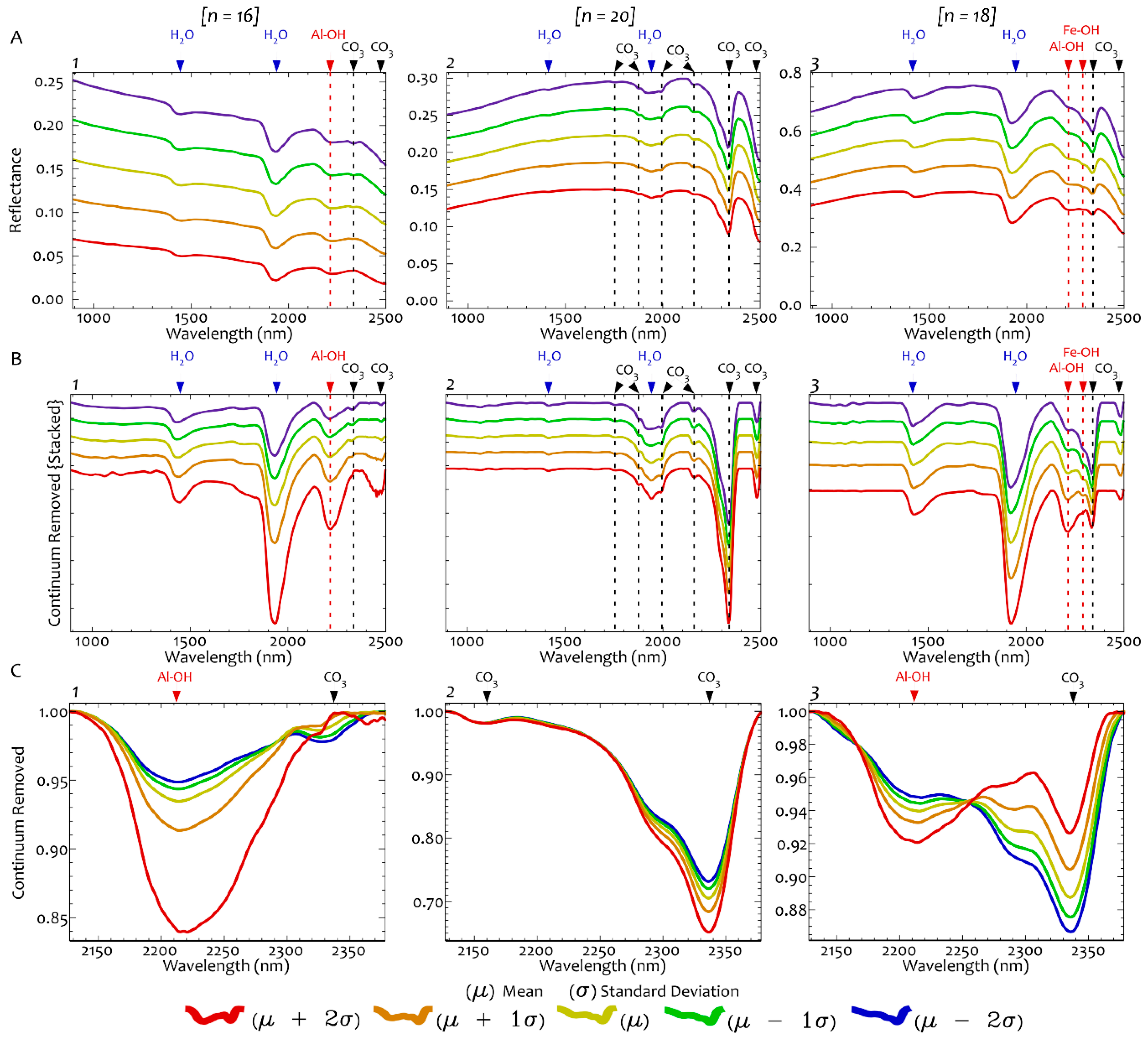
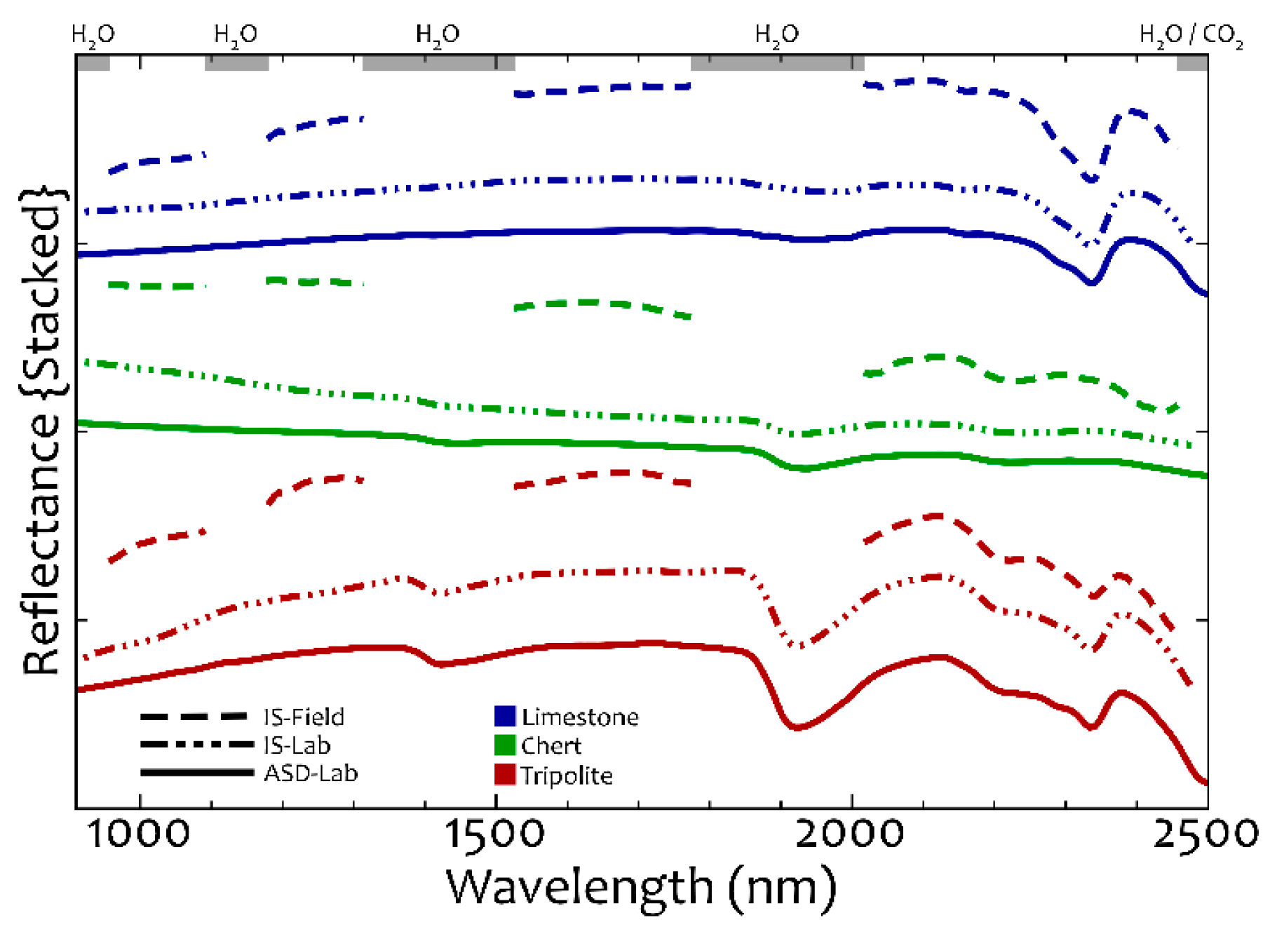
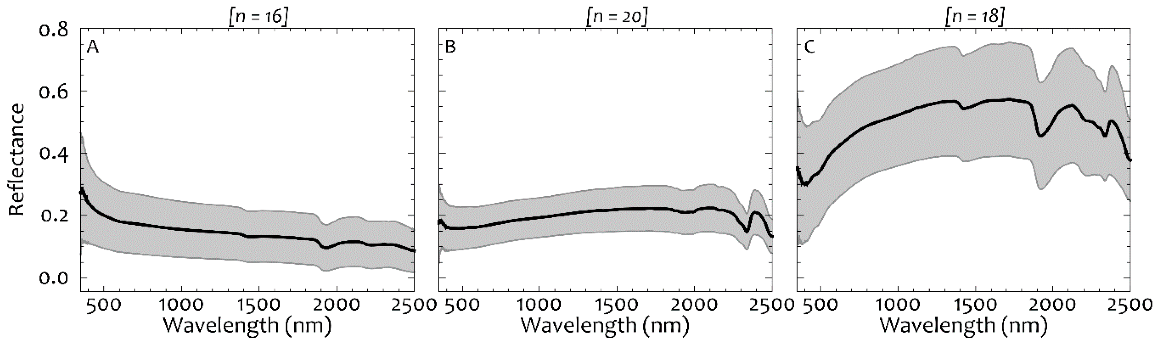
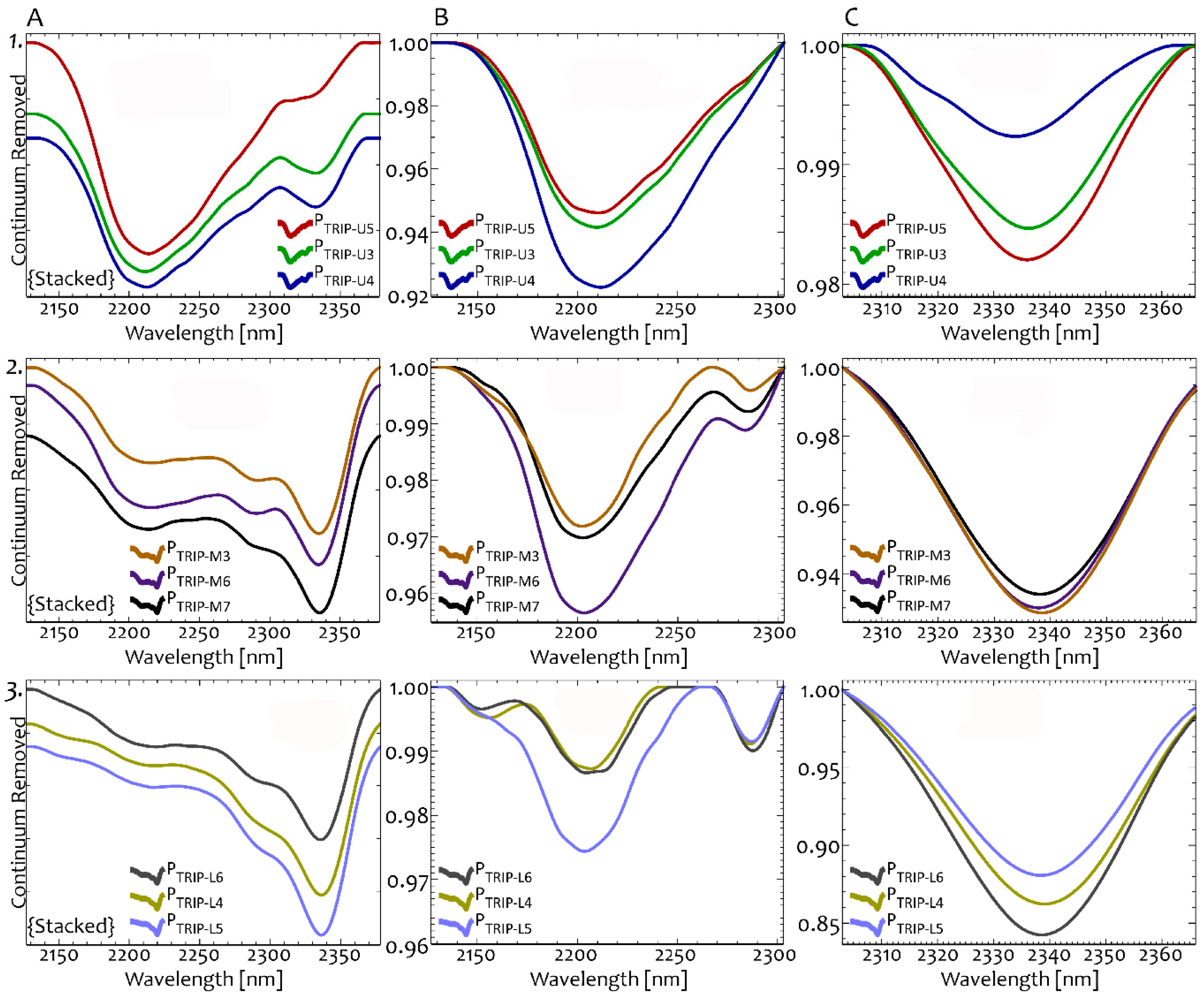
3.1. Laboratory Reflectance Spectroscopy
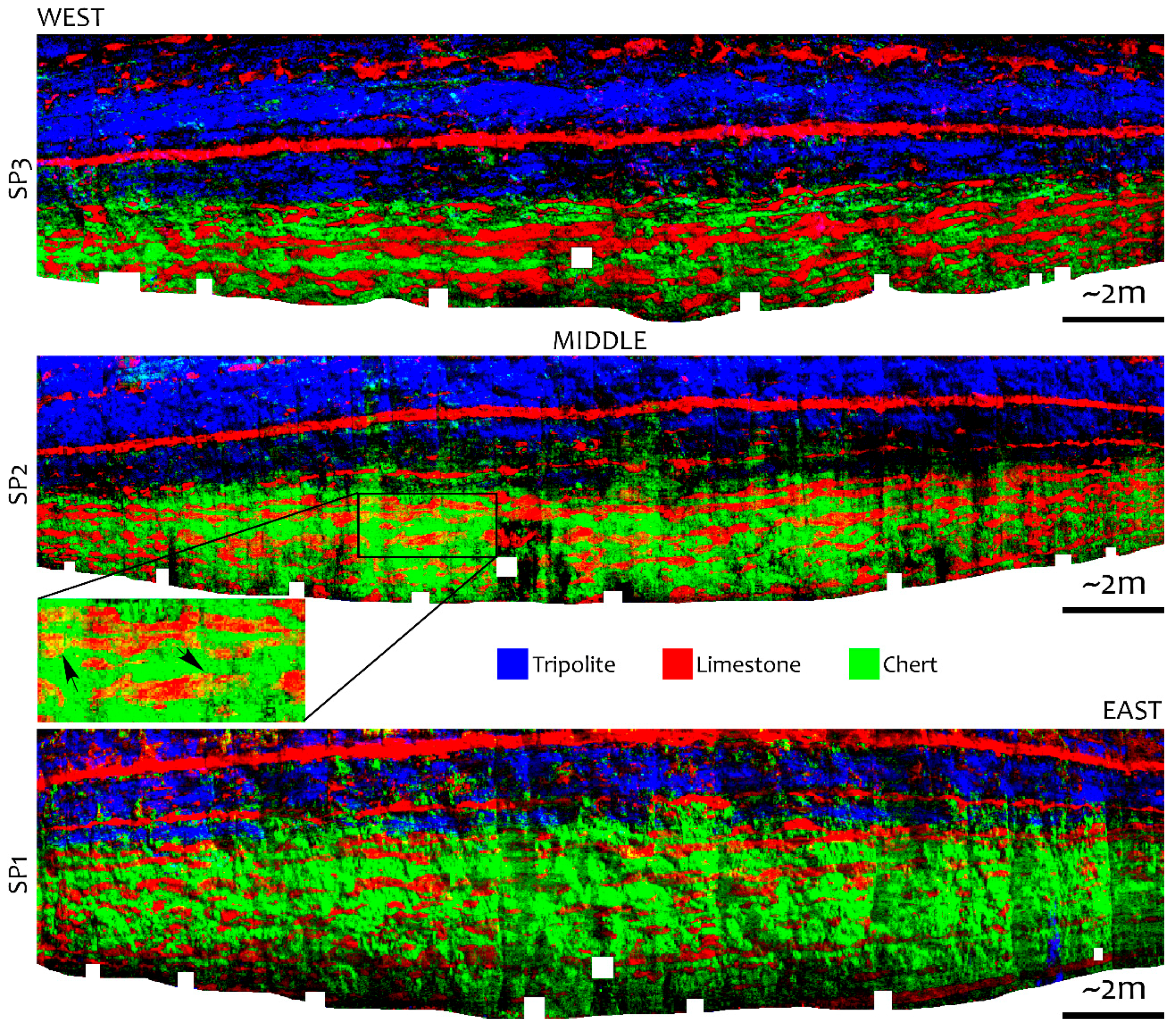
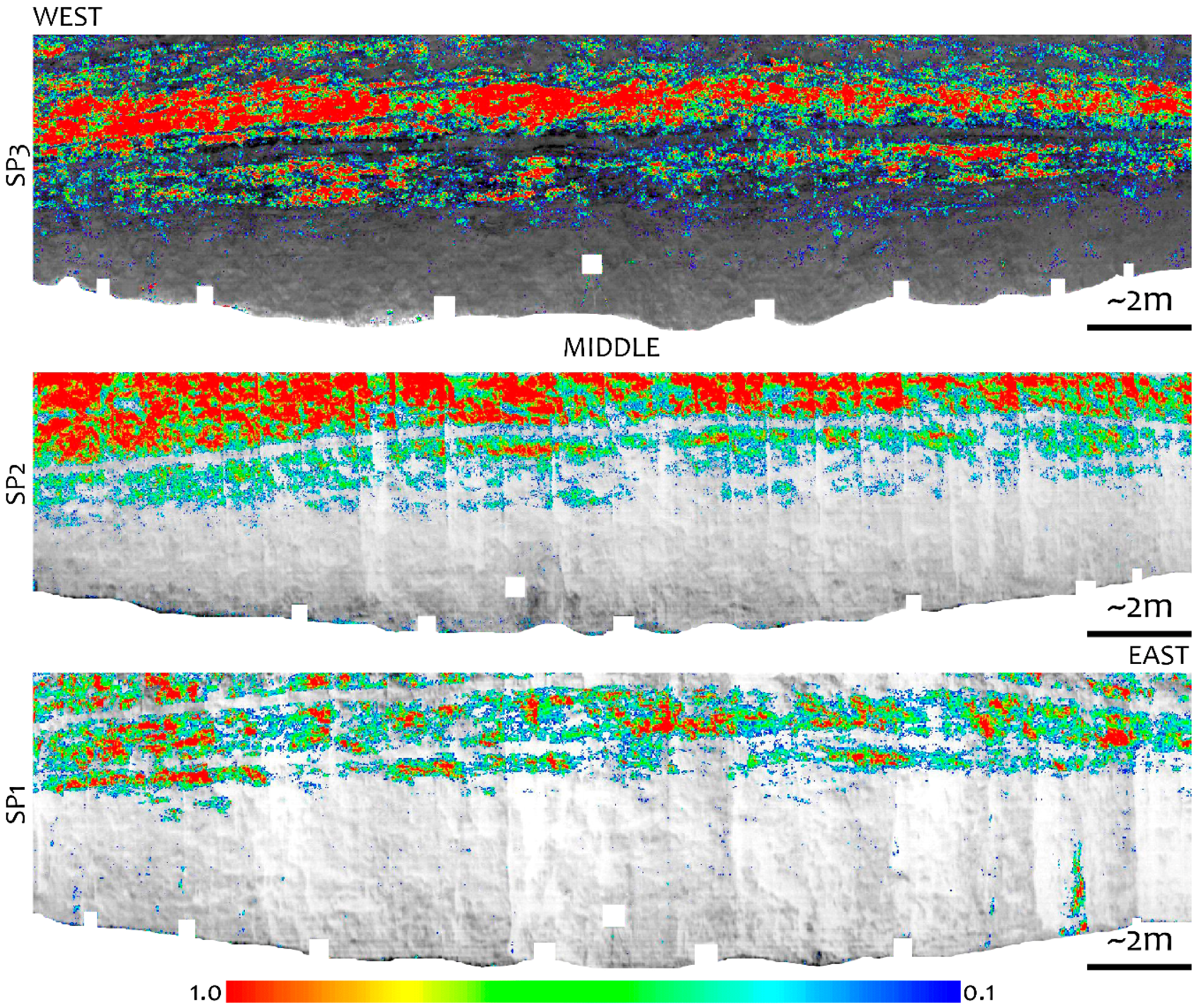
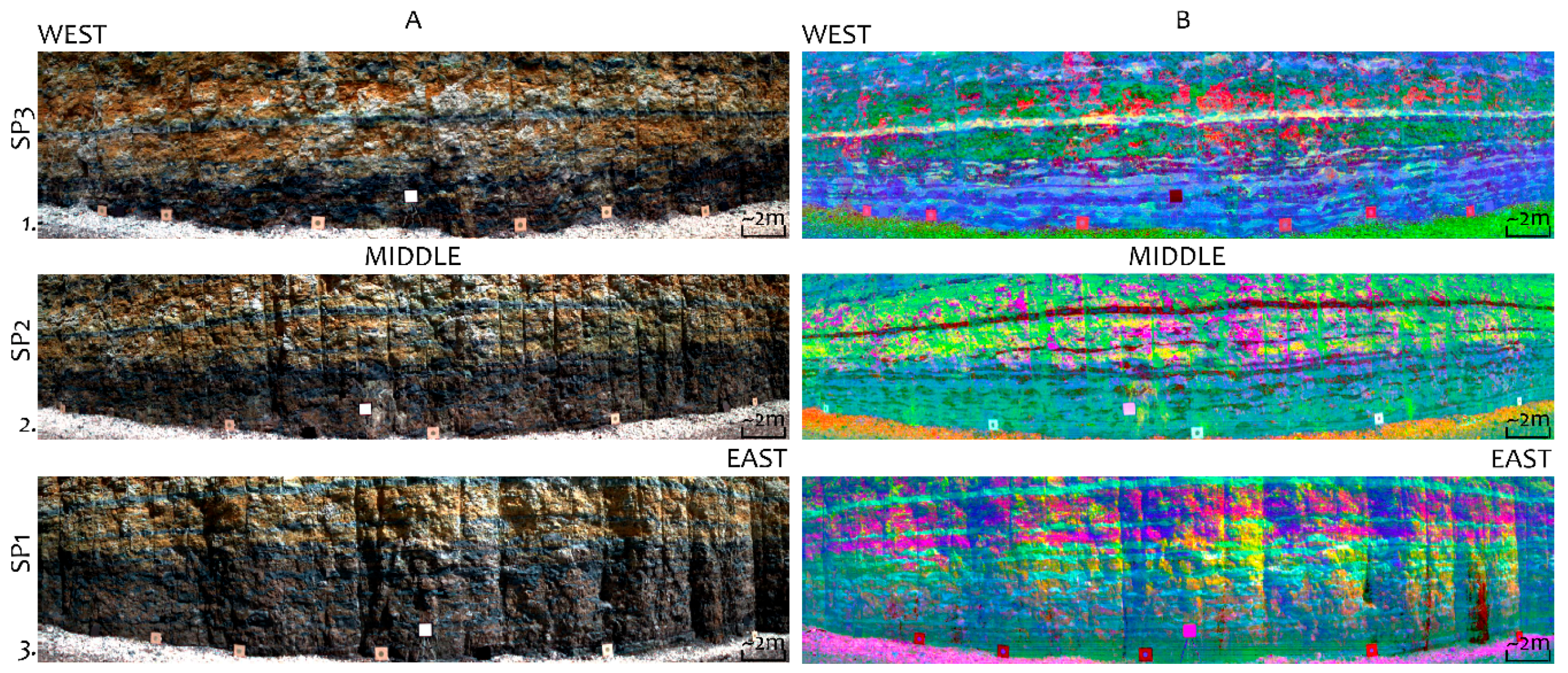
3.2. Hyperspectral Image Classification
4. Discussion
5. Conclusions
Acknowledgments
Author Contributions
Conflicts of Interest
References
- Gigli, G.; Casagli, N. Semi-automatic extraction of rock mass structural data from high resolution LIDAR point clouds. Int. J. Rock Mech. Min. Sci. 2011, 48, 187–198. [Google Scholar] [CrossRef]
- Matano, F.; Iuliano, S.; Somma, R.; Marino, E.; del Vecchio, U.; Esposito, G.; Mollisso, F.; Scepi, G.; Grimaldi, G.M.; Pignalosa, A. Geostructure of Coroglio tuff cliff, Naples (Italy) derived from terrestrial laser scanner data. J. Maps 2016. [Google Scholar] [CrossRef]
- Xu, X.; Aiken, C.L.V.; Bhattacharya, J.P.; Corbeanu, R.M.; Nielsen, K.C.; McMechan, G.A.; Abdelsalam, M.G. Creating virtual 3-D outcrop. Lead Edge 2000, 19, 197–202. [Google Scholar] [CrossRef]
- Bellian, J.A. Digital outcrop models: Applications of terrestrial scanning lidar technology in stratigraphic modeling. J. Sediment. Res. 2005, 75, 166–176. [Google Scholar] [CrossRef]
- Buckley, S.J.; Schwarz, E.; Terlaky, V.; Howell, J.A.; Arnott, R.W. Combining aerial photogrammetry and terrestrial lidar for reservoir analog modeling. Photogramm. Eng. Remote Sens. 2010, 76, 953–963. [Google Scholar] [CrossRef]
- Enge, H.D.; Buckley, S.J.; Rotevatn, A.; Howell, J.A. From outcrop to reservoir simulation model: Workflow and procedures. Geosphere 2007, 3, 469–490. [Google Scholar] [CrossRef]
- Humair, F.; Abellan, A.; Carrea, D.; Matasci, B.; Epard, J.L.; Jaboyedoff, M. Geological layers detection and characterisation using high resolution 3D point clouds: Example of a box-fold in the Swiss Jura Mountains. Eur. J. Remote Sens. 2015, 48, 541–568. [Google Scholar] [CrossRef]
- Bowen, B.B.; Martini, B.A.; Chan, M.A.; Parry, W.T. Reflectance spectroscopic mapping of diagenetic heterogeneities and fluid-flow pathways in the Jurassic Navajo Sandstone. Am. Assoc. Pet. Geol. Bull. 2007, 91, 173–190. [Google Scholar] [CrossRef]
- Bell, J.H.; Bowen, B.B.; Martini, B.A. Imaging spectroscopy of jarosite cement in the Jurassic Navajo Sandstone. Remote Sens. Environ. 2010, 114, 2259–2270. [Google Scholar] [CrossRef]
- Asadzadeh, S.; de Souza, F.C.R. A review on spectral processing methods for geological remote sensing. Int. J. Appl. Earth Obs. Geoinf. 2016, 47, 69–90. [Google Scholar] [CrossRef]
- Hunt, G.R. Spectral signatures of particulate minerals in the vivible and near infrared. Geophysics 1977, 42, 501–513. [Google Scholar] [CrossRef] [Green Version]
- Clark, R.N.; King, T.V.V.; Klejwa, M.; Swayze, G.A.; Vergo, N. High spectral resolution reflectance spectroscopy of minerals. J. Geophys. Res. 1990, 95, 12612–12680. [Google Scholar] [CrossRef]
- Bellian, J.A.; Beck, R.; Kerans, C. Analysis of hyperspectral and lidar data: Remote optical mineralogy and fracture identification. Geosphere 2007, 3, 491–500. [Google Scholar] [CrossRef]
- Huntington, J.F.; Mauger, A.J.; Skirrow, R.G.; Bastrakov, E.N.; Connor, P.; Mason, P.; Keeling, J.L.; Coward, D.A.; Berman, M.; Phillips, R.; et al. Automated mineralogical core logging at the Emmie Bluff iron oxide-copper-gold prospect. MESA J. 2006, 41, 38–44. [Google Scholar]
- Mauger, A.J. Mapping regional alteration patterns using hyperspectral drillcore scanner. ASEG Ext. Abstr. 2007. [Google Scholar] [CrossRef]
- Kruse, F.A.; Bedell, R.L.; Taranik, J.V.; Peppin, W.A.; Weatherbee, O.; Calvin, W.M. Mapping alteration minerals at prospect, outcrop and drill core scales using imaging spectrometry. Int. J. Remote Sens. 2012, 33, 1780–1798. [Google Scholar] [CrossRef] [PubMed]
- Kurz, T.H.; Dewit, J.; Buckley, S.J.; Thurmond, J.B.; Hunt, D.W.; Swennen, R. Hyperspectral image analysis of different carbonate lithologies (limestone, karst and hydrothermal dolomites): The Pozalagua Quarry case study (Cantabria, North-west Spain). Sedimentology 2012, 59, 623–645. [Google Scholar] [CrossRef]
- Murphy, R.J.; Schneider, S.; Monteiro, S.T. Mapping layers of clay in a vertical geological surface using hyperspectral imagery: Variability in parameters of SWIR absorption features under different conditions of illumination. Remote Sens. 2014, 6, 9104–9129. [Google Scholar] [CrossRef]
- Okyay, U.; Khan, S.D. Remote detection of fluid-related diagenetic mineralogical variations in the Wingate Sandstone at different spatial and spectral resolutions. Int. J. Appl. Earth Obs. Geoinf. 2016, 44, 70–87. [Google Scholar] [CrossRef]
- Snyder, C.J.; Khan, S.D.; Bhattacharya, J.P.; Glennie, C.; Seepersad, D. Thin-bedded reservoir analogs in an ancient delta using terrestrial laser scanner and high-resolution ground-based hyperspectral cameras. Sediment. Geol. 2016, 342, 154–164. [Google Scholar] [CrossRef]
- Krupnik, D.; Khan, S.; Okyay, U.; Hartzell, P.; Zhou, H.-W. Study of Upper Albian rudist buildups in the Edwards Formation using ground-based hyperspectral imaging and terrestrial laser scanning. Sediment. Geol. 2016, 345, 154–167. [Google Scholar] [CrossRef]
- Sun, L.; Khan, S. Ground-based hyperspectral remote sensing of hydrocarbon-induced rock alterations at cement, Oklahoma. Mar. Pet. Geol. 2016, 77, 1243–1253. [Google Scholar] [CrossRef]
- Zaini, N.; Van der Meer, F.D.; van der Werff, H.M.A. Determination of carbonate rock chemistry using laboratory-based hyperspectral imagery. Remote Sens. 2014, 6, 4149–4172. [Google Scholar] [CrossRef]
- Greenberger, R.N.; Mustard, J.F.; Cloutis, E.A.; Mann, P.; Wilson, J.H.; Flemming, R.L.; Robertson, K.M.; Salvatore, M.R.; Edwards, C.S. Hydrothermal alteration and diagenesis of terrestrial lacustrine pillow basalts: Coordination of hyperspectral imaging with laboratory measurements. Geochim. Cosmochim. Acta 2015, 171, 174–200. [Google Scholar] [CrossRef]
- Mazzullo, S.J.J.; Boardman, D.R.; Wilhite, B.W.; Godwin, C.J.; Morris, B.T. Revisions of outcrop lithostratigraphic nomenclature in the Lower to Middle Mississippian Subsystem (Kinderhookian to Basal Meramecian series) along the shelf-edge in southwest Missouri, northwest Arkansas, and northeast Oklahoma. Shale Shak 2013, 63, 414–454. [Google Scholar]
- Gutschick, R.; Sandberg, C. Mississippian continental margins on the conterminous United States. SEPM Spec. Publ. 1983, 33, 79–96. [Google Scholar]
- Montgomery, S.L.; Mullarkey, J.C.; Longman, M.W.; Colleary, W.M.; Rogers, J.P. Mississippian “chat” reservoirs, South Kansas: Low-resistivity pay in a complex chert reservoir. Am. Assoc. Pet. Geol. Bull. 1998, 82, 187–205. [Google Scholar] [CrossRef]
- Watney, W.L.; Guy, W.J.; Byrnes, A.P. Characterization of the Mississippian chat in south-central Kansas. Am. Assoc. Pet. Geol. Bull. 2001, 85, 85–113. [Google Scholar]
- Elebiju, O.O.; Matson, S.; Keller, R.G.; Marfurt, K.J. Integrated geophysical studies of the basement structures, the Mississippi chert, and the Arbuckle Group of Osage County region, Oklahoma. Am. Assoc. Pet. Geol. Bull. 2011, 95, 371–393. [Google Scholar] [CrossRef]
- Mazzullo, S.J.; Wilhite, B.W.; Boardman, D.R.; Morris, B.T.; Godwin, C.J. Stratigraphic architecture and petroleum reservoirs in Lower to Middle Mississippian strata (Kinderhookian to basal Meramecian) in subsurface Central to southern Kansas and northern Oklahoma. Shale Shak 2016, 67, 20–49. [Google Scholar]
- Mazzullo, S.J.; Wilhite, B.W.; Boardman, D.R. Lithostratigraphic architecture of the Mississippian Reeds Springs Formation (Middle Osagean) in southwest Missouri, northwest Arkansas, and northeast Oklahoma: Outcrop analog of subsurface petroleum reservoirs. Shale Shak 2011, 61, 254–269. [Google Scholar]
- Heckel, P.H. Carboniferous Period. In A Concise Geologic Time Scale; Ogg, J.G., Ogg, G., Gradstein, F.M., Eds.; Cambridge University Press: Cambridge, UK, 2008; pp. 73–83. [Google Scholar]
- Richards, B.C. Current status of the international carboniferous time scale. In Carboniferous-Permian Transition. New Mexico Museum of Natural History and Science Bulletin 60; Lucas, S.G., DiMichele, W.A., Barrick, J.E., Schneider, J.W., Spielmann, J.A., Eds.; New Mexico Museum of Natural History: Albuquerque, NM, USA, 2013; pp. 348–353. [Google Scholar]
- Lane, H.R.; De Keyser, T.L. Paleogeography of the Late Early Mississippian (Tournaisian 3) in the central and southwestern United States. In Paleozoic Paleogeography of the West-Central United States; Fouch, T.D., Magathan, E.R., Eds.; The Rocky Mountain Section SEPM: Denver, CO, USA, 1980; pp. 149–162. [Google Scholar]
- Manger, W.L.; Shelby, P.R. Natural-gas production from the Boone Formation (Lower Mississippian), northwestern Arkansas. In Proceedings of the Platform Carbonates in the Southern Midcontinent, 1996 Symposium, Oklahoma City, OK, USA, 26–27 March 1996.
- Thompson, T.L. Paleozoic Succession in Missouri, Part 4 Mississippian System; Missouri Department of Natural Resources: Jefferson City, MS, USA, 1986.
- Mazzullo, S.J. My favorite outcrop—Mississippian tripolite. Shale Shak 2015, 66, 147–149. [Google Scholar]
- Color, M. Geological Rock-Color Chart; X-rite Munsell Color: Grand Rapids, MI, USA, 2009. [Google Scholar]
- Minor, P.M. Analysis of tripolitic chert in the Boone Formation (Lower Mississippian, Osagean), northwest Arkansas and southwestern Missouri. Master’s Thesis, University of Arkansas, Fayetteville, AR, USA, 2013. [Google Scholar]
- Mazzullo, S.J.; Wilhite, B.W. Chert, tripolite, spiculite, chat-what’s in a name? Kansas Geol. Soc. Bull. 2010, 85, 21–25. [Google Scholar]
- Keller, W.D. Textures of tripoli illustrated by scanning electron micrographs. Econ. Geol. 1978, 73, 442–446. [Google Scholar] [CrossRef]
- Satterwhite, M.B.; Allen, C.S. A novel, low cost approach for large gray-toned fabric panels for calibrating remotely sensed VIS/NIR/SWIR data. Proc. SPIE 2003, 5093, 163–171. [Google Scholar] [CrossRef]
- Rochford, P.A.; Acharya, P.K.; Adler-Golden, S.M.; Berk, A.; Bernstein, L.S.; Matthew, M.W.; Richtsmeier, S.C.; Gulick, S.; Slusser, J. Validation and refinement of hyperspectral/multispectral atmospheric compensation using shadowband radiometers. IEEE Trans. Geosci. Remote Sens. 2005, 43, 2898–2906. [Google Scholar] [CrossRef]
- Kurz, T.H.; Buckley, S.J.; Howell, J.A. Close-range hyperspectral imaging for geological field studies: Workflow and methods. Int. J. Remote Sens. 2013, 34, 1798–1822. [Google Scholar] [CrossRef]
- Nieke, J.; Schläpfer, D.; Dell’Endice, F.; Brazile, J.; Itten, K.I. Uniformity of imaging spectrometry data products. IEEE Trans. Geosci. Remote Sens. 2008, 46, 3326–3336. [Google Scholar] [CrossRef] [Green Version]
- Watson, K. Processing remote sensing images using the 2-D FFT-noise reduction and other applications. Geophysics 1993, 58, 835–852. [Google Scholar] [CrossRef]
- Kennedy, R.E.; Cohen, W.B.; Takao, G. Empirical methods to compensate for a view-angle-dependent brightness gradient in AVIRIS imagery. Remote Sens. Environ. 1997, 62, 277–291. [Google Scholar] [CrossRef]
- Schiefer, S.; Hostert, P.; Damm, A. Correcting brightness gradients in hyperspectral data from urban areas. Remote Sens. Environ. 2006, 101, 25–37. [Google Scholar] [CrossRef]
- Smith, G.M.; Milton, E.J. The use of the empirical line method to calibrate remotely sensed data to reflectance. Int. J. Remote Sens. 1999, 20, 2653–2662. [Google Scholar] [CrossRef]
- Savitzky, A.; Golay, M.J.E. Smoothing and differentiation of data by simplified least squares procedures. Anal. Chem. 1964, 36, 1627–1639. [Google Scholar] [CrossRef]
- Ruffin, C.; King, R. The analysis of hyperspectral data using Savitzky-Golay filtering—Theoretical basis (Part 1). In Proceedings of the IEEE 1999 International Geoscience and Remote Sensing Symposium, Hamburg, Germany, 28 June–2 July 1999.
- Green, A.A.; Berman, M.; Switzer, P.; Craig, M.D. Transformation for ordering multispectral data in terms of image quality with implications for noise removal. IEEE Trans. Geosci. Remote Sens. 1988, 26, 65–74. [Google Scholar] [CrossRef]
- Atkinson, P.M.; Sargent, I.M.; Foody, G.M.; Williams, J. Interpreting image-based methods for estimating the signal-to-noise ratio. Int. J. Remote Sens. 2005, 26, 5099–5115. [Google Scholar] [CrossRef]
- van der Meer, F.D.; de Jong, S.M.; Bakker, W.H. Imaging spectrometry: Basic analytical techniques. In Imaging Spectrom: Basic Principles and Prospective Applications; Van Der Meer, F.D., de Jong, S.M., Eds.; Springer: Dordrecht, The Netherlands, 2001; pp. 17–61. [Google Scholar]
- Clark, R.N.; Gallagher, A.J.; Swayze, G.A. Material absorption band depth mapping of imaging spectrometer data using a complete band shape least-squares fit with library reference spectra. In Proceedings of the Second Airborne Visible/Infrared Imaging Spectrometer Workshop, Pasadena, CA, USA, 4–5 June 1990; pp. 176–186.
- Clark, R.N.; Swayze, G.A.; Gallagher, A.J.; Gorelick, N.; Kruse, F.A. Mapping with imaging spectrometer data using the complete band shape least-squares algorithm simultaneously fit to multiple spectral features from multiple materials. In Proceedings of the Third Airborne Visible/Infrared Imaging Spectrometer Workshop, Pasadena, CA, USA, 20–21 May 1991; pp. 2–3.
- Harsanyi, J.C.; Chang, C.I. Hyperspectral image classification and dimensionality reduction: An orthogonal subspace projection approach. IEEE Trans. Geosci. Remote Sens. 1994, 32, 779–785. [Google Scholar] [CrossRef]
- Boardman, J.W.; Kruse, F.A.; Green, R.O. Mapping target signatures via partial unmixing of AVIRIS data. In Proceedings of the 5th JPL Airborne Earth Science Workshop, Pasadena, CA, USA, 23–26 January 1995; pp. 23–26.
- Boardman, J.W. Leveraging the high dimensionality of AVIRIS data for improved sub-pixel target unmixing and rejection of false positives: mixture tuned matched filtering. In Proceedings of the 7th JPL Airborne Earth Science Workshop, Pasadena, CA, USA, 12–16 January 1998; pp. 55–56.
- Debba, P.; Van Ruitenbeek, F.J.A.; Van Der Meer, F.D.; Carranza, E.J.M.; Stein, A. Optimal field sampling for targeting minerals using hyperspectral data. Remote Sens. Environ. 2005, 99, 373–386. [Google Scholar] [CrossRef]
- Pan, Z.; Huang, J.; Wang, F. Multi range spectral feature fitting for hyperspectral imagery in extracting oilseed rape planting area. Int. J. Appl. Earth Obs. Geoinf. 2013, 25, 21–29. [Google Scholar] [CrossRef]
- van der Meer, F.D. Analysis of spectral absorption features in hyperspectral imagery. Int. J. Appl. Earth Obs. Geoinf. 2004, 5, 55–68. [Google Scholar] [CrossRef]
- Tangestani, M.H.; Jaffari, L.; Vincent, R.K.; Sridhar, B.B.M. Spectral characterization and ASTER-based lithological mapping of an ophiolite complex: A case study from Neyriz ophiolite, SW Iran. Remote Sens. Environ. 2011, 115, 2243–2254. [Google Scholar] [CrossRef]
- Kruse, F.A.; Boardman, J.W.; Huntington, J.F. Comparison of airborne hyperspectral data and EO-1 Hyperion for mineral mapping. IEEE Trans. Geosci. Remote Sens. 2003, 41, 1388–1400. [Google Scholar] [CrossRef]
- Nidamanuri, R.R.; Zbell, B. Use of field reflectance data for crop mapping using airborne hyperspectral image. ISPRS J. Photogramm. Remote Sens. 2011, 66, 683–691. [Google Scholar] [CrossRef]
- Clark, R.N. Spectroscopy of rocks and minerals, and principles of spectroscopy. Man. Remote Sens. 1999, 3, 3–58. [Google Scholar] [CrossRef]
- Gaffey, S.J. Reflectance spectroscopy in the visible and near-infrared (0.35–2.55 µm): Applications in carbonate petrology. Geology 1985, 13, 270. [Google Scholar] [CrossRef]
- Sherman, D.M.; Waite, T.D. Electronic spectra of Fe3+ oxides and oxide hydroxides in the near IR to near UV. Am. Mineral. 1985, 70, 1262–1269. [Google Scholar]
- Chabrillat, S.; Goetz, A.F.H.; Olsen, H.W.; Krosley, L. Field and imaging spectrometry for identification and mapping of expansive soils. In Basic Principles and Prospective Applications: Imaging Spectrometry; van der Meer, F.D., de Jong, S.M., Eds.; Springer: Dordrecht, The Netherlands, 2001; pp. 87–109. [Google Scholar]
- Gupta, R.P. Spectra of minerals and rocks. In Remote Sensing Geology, 2nd ed.; Springer: Berlin/Heidelberg, Germany, 2003; pp. 33–52. [Google Scholar]
- Gaffey, S.J. Spectral reflectance of carbonate minerals in the visible and near infrared (0.35–2.55 microns): Calcite, aragonite, and dolomite. Am. Mineral. 1986, 71, 151–162. [Google Scholar]
- Bishop, J.L.; Lane, M.D.; Dyar, M.D.; Brown, A.J. Reflectance and emission spectroscopy study of four groups of phyllosilicates: Smectites, kaolinite-serpentines, chlorites and micas. Clay Miner. 2008, 43, 35–54. [Google Scholar] [CrossRef]
- Harris, J.R.; Rogge, D.; Hitchcock, R.; Ijewliw, O.; Wright, D. Mapping lithology in Canada’s Arctic: Application of hyperspectral data using the minimum noise fraction transformation and matched filtering. Can. J. Earth Sci. 2005, 42, 2173–2193. [Google Scholar] [CrossRef]
- Manger, W.L. Tripolitic chert development in the Mississippian lime: New insights from SEM. In Presented at Mississippian Lime Play Forum, Oklahoma City, OK, USA, 20 February 2014.
- Christopher, J.E. The Lower Cretaceous Mannville Group, northern Williston Basin region, Canada. In The Mesozoic of Middle North America: A Selection of Papers from the Symposium on the Mesozoic of Middle North America, Calgary, Alberta, Canada—Memoir 9, 1984; Canadian Society of Petroleum Geologists: Calgary, AB, Canada, 1984; Volume 9, pp. 109–126. [Google Scholar]
- Christopher, J.E. The Lower Cretaceous Mannville group of Saskatchewan—A tectonic overview. Saskatchewan Geol. Soc. Spec. Publ. 1980, 5, 3–32. [Google Scholar]
- Swanson, R.G. Sample Examination Manual; American Association of Petroleum Geologists: Tulsa, Ok, USA, 1981. [Google Scholar]


| VNIR Camera | SWIR Camera | |
|---|---|---|
| Spectrograph | ImSpector V10E | ImSpector N25E |
| Spectral range | 400–1000 nm | 900–2500 nm |
| Spectral Sampling | 0.72–5.8 nm 1 | 6.3 nm |
| Sensor | HgCdTe (MCT) | Charged-couple device(CCD) |
| Spatial dimension | 1600 pixels 2 | 320 pixels |
| Spectral dimension | 840 pixels 1 | 256 pixels |
| Pixel pitch | 7.4 µm | 30 µm |
| Digitization | 12-bit | 14-bit |
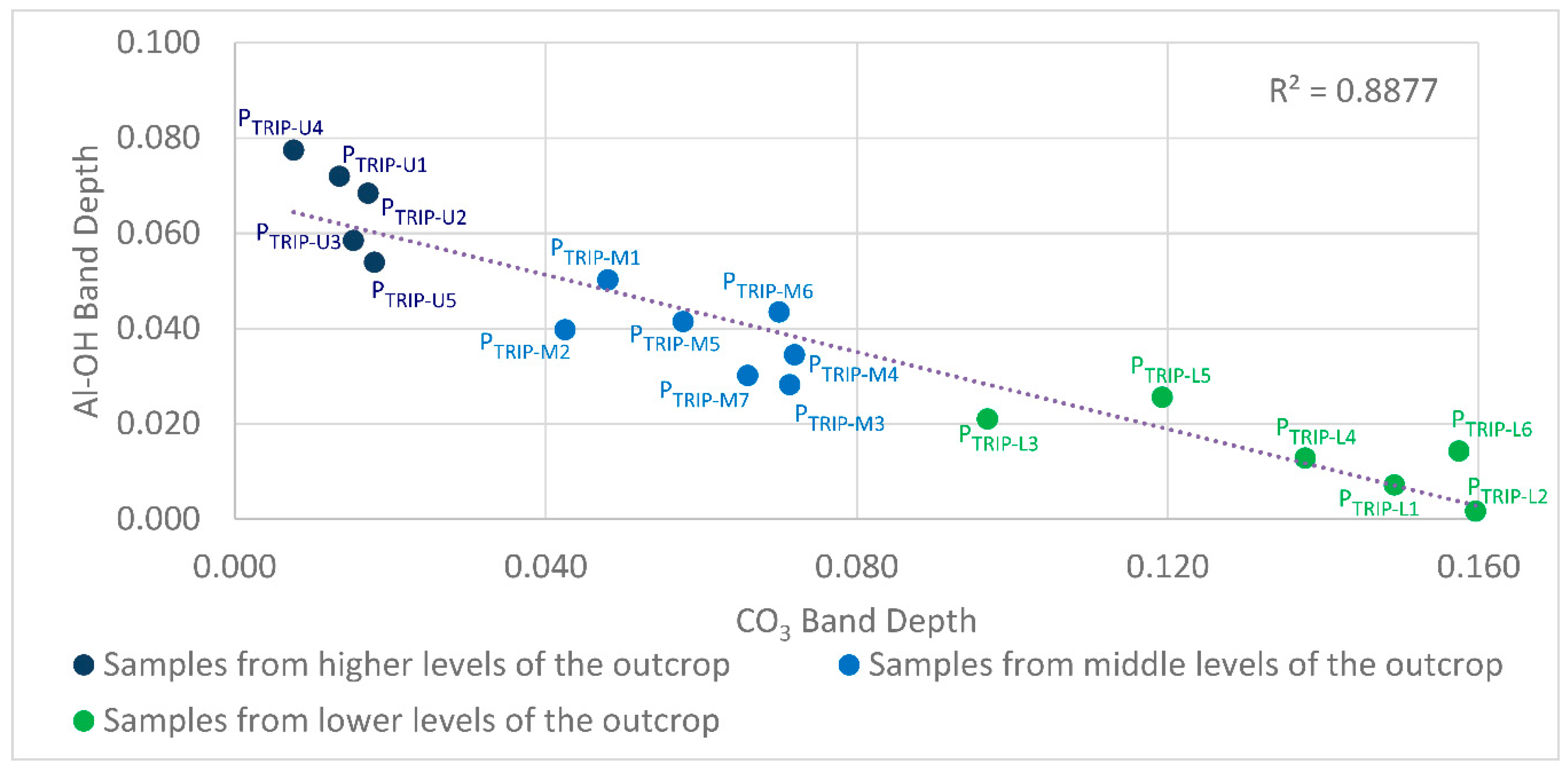
| Tripolite Sample Number | Continuum Removed over 2128–2302 nm Wavelength Range | Continuum Removed over 2303–2373 nm Wavelength Range | ||
|---|---|---|---|---|
| Al-OH Absorption Feature around 2210 nm | CO3 Absorption Feature around 2340 nm | |||
| Wavelength Position [nm] | Absorption Depth | Wavelength Position [nm] | Absorption Depth | |
| PTRIP-U5 | 2210 | 0.05390 | 2336 | 0.01800 |
| PTRIP-U4 | 2211 | 0.07750 | 2335 | 0.00760 |
| PTRIP-U3 | 2210 | 0.05850 | 2337 | 0.01530 |
| PTRIP-U2 | 2212 | 0.06840 | 2335 | 0.01720 |
| PTRIP-U1 | 2211 | 0.07200 | 2335 | 0.01350 |
| PTRIP-M7 | 2208 | 0.03020 | 2338 | 0.06600 |
| PTRIP-M6 | 2207 | 0.04350 | 2338 | 0.07000 |
| PTRIP-M5 | 2207 | 0.04150 | 2339 | 0.05770 |
| PTRIP-M4 | 2207 | 0.03450 | 2338 | 0.07200 |
| PTRIP-M3 | 2208 | 0.02820 | 2338 | 0.07140 |
| PTRIP-M2 | 2208 | 0.03980 | 2337 | 0.04250 |
| PTRIP-M1 | 2209 | 0.05020 | 2337 | 0.04800 |
| PTRIP-L6 | 2209 | 0.01430 | 2338 | 0.15750 |
| PTRIP-L5 | 2207 | 0.02560 | 2339 | 0.11930 |
| PTRIP-L4 | 2207 | 0.01280 | 2339 | 0.13770 |
| PTRIP-L3 | 2208 | 0.02100 | 2339 | 0.09680 |
| PTRIP-L2 | 2215 | 0.00170 | 2339 | 0.15960 |
| PTRIP-L1 | 2208 | 0.00720 | 2339 | 0.14920 |
© 2016 by the authors; licensee MDPI, Basel, Switzerland. This article is an open access article distributed under the terms and conditions of the Creative Commons Attribution (CC-BY) license (http://creativecommons.org/licenses/by/4.0/).
Share and Cite
Okyay, Ü.; Khan, S.D.; Lakshmikantha, M.R.; Sarmiento, S. Ground-Based Hyperspectral Image Analysis of the Lower Mississippian (Osagean) Reeds Spring Formation Rocks in Southwestern Missouri. Remote Sens. 2016, 8, 1018. https://doi.org/10.3390/rs8121018
Okyay Ü, Khan SD, Lakshmikantha MR, Sarmiento S. Ground-Based Hyperspectral Image Analysis of the Lower Mississippian (Osagean) Reeds Spring Formation Rocks in Southwestern Missouri. Remote Sensing. 2016; 8(12):1018. https://doi.org/10.3390/rs8121018
Chicago/Turabian StyleOkyay, Ünal, Shuhab D. Khan, M. R. Lakshmikantha, and Sergio Sarmiento. 2016. "Ground-Based Hyperspectral Image Analysis of the Lower Mississippian (Osagean) Reeds Spring Formation Rocks in Southwestern Missouri" Remote Sensing 8, no. 12: 1018. https://doi.org/10.3390/rs8121018