Article

Water Budget Analysis within the Surrounding of Prominent Lakes and Reservoirs from Multi-Sensor Earth Observation Data and Hydrological Models: Case Studies of the Aral Sea and Lake Mead

1
Deutsches Geodätisches Forschungsinstitut (DGFI-TUM), Technische Universität München, Arcisstr. 21, Munich 80333, Germany
2
HafenCity Universität, Überseeallee 16, Hamburg 20457, Germany
3
Helmholtz Center Potsdam, GFZ German Research Centre for Geosciences, Telegrafenberg, Potsdam 14473, Germany
4
Institute of Earth and Environmental Science, University of Potsdam, Potsdam 14476, Germany
*
Author to whom correspondence should be addressed.
Remote Sens. 2016, 8(11), 953; https://doi.org/10.3390/rs8110953
Submission received: 22 August 2016 / Revised: 20 October 2016 / Accepted: 8 November 2016 / Published: 16 November 2016
(This article belongs to the Special Issue Remote Sensing of Climate Change and Water Resources)

Abstract

:
The hydrological budget of a region is determined based on the horizontal and vertical water fluxes acting in both inward and outward directions. These integrated water fluxes vary, altering the total water storage and consequently the gravitational force of the region. The time-dependent gravitational field can be observed through the Gravity Recovery and Climate Experiment (GRACE) gravimetric satellite mission, provided that the mass variation is above the sensitivity of GRACE. This study evaluates mass changes in prominent reservoir regions through three independent approaches viz. fluxes, storages, and gravity, by combining remote sensing products, in-situ data and hydrological model outputs using WaterGAP Global Hydrological Model (WGHM) and Global Land Data Assimilation System (GLDAS). The results show that the dynamics revealed by the GRACE signal can be better explored by a hybrid method, which combines remote sensing-based reservoir volume estimates with hydrological model outputs, than by exclusive model-based storage estimates. For the given arid/semi-arid regions, GLDAS based storage estimations perform better than WGHM.

1. Introduction

Eighty-seven percent of Earth’s open freshwater is stored in reservoirs (here, the term reservoir includes both lakes and man-made reservoirs), 2% is stored in rivers and the remaining 11% in swamps [1]. Timely and accurate knowledge of water conditions and dynamics in reservoirs and their contributing catchment areas provide a basis for efficient and sustainable management of water resources, as well as to prepare for its inevitable future variability. Water storage can be regularly quantified by applying: ground-based observations, hydrological modeling and remote sensing [2,3]. Given the decreasing number of ground-based gauging stations around the globe [4,5] and the uncertainty of hydrological models [6], the application of diverse remote sensing based technologies must be fostered. Remote sensing has provided a rich database for water-related parameters and state variables. The combination or assimilation of ground-based data and remote sensing products into models can provide extensive and more precise information about regional water resources. This study evaluates the potential of hybrid products in a reservoir-dominated region by combining model outputs, ground-based data, and remote sensing data.
Large variations in water mass change the gravity field of a region and thus map into the observations of the Gravity Recovery and Climate Experiment (GRACE) satellite mission. The study interprets the impact of reservoir dynamics on the GRACE signal. Since the resolution of GRACE is limited to large signals and regions, an appropriate window around the reservoir needs to be selected and other hydrological parameters need to be quantified. The water balance equation within a region can be recognized as a series of fluxes and storages (stocks). To observe this regional water budget variability, we have applied the following approaches:
  • Estimation of the balance of all hydrological fluxes acting vertically and horizontally. The rate of water storage change (ΔS/dt) in a region is the sum of evapotranspiration (ET), precipitation (P) and net surface runoff (ΔR) Equation (1),
    ΔS/dt = P − ET + ΔR
    Based on the applied datasets, two net fluxes are derived from Equation (1). Flux-1 is obtained by combining the Global Precipitation Climatology Centre (GPCC) precipitation data with the WaterGAP Global Hydrological Model (WGHM) ET and in-situ runoff. Flux-2 is obtained by combining the Tropical Rainfall Measuring Mission (TRMM-3B43) precipitation data with the Global Land Data Assimilation System (GLDAS) ET and in-situ runoff.
  • Estimation of the water storage change (ΔS) in a region is the sum of storages in soil moisture (SM), snow water equivalent (SWE) and surface water (SW) (Equation (2)). Due to the lack of direct measurements, groundwater storage is not considered in the equation.
    ΔS = ΔSM + ΔSWE + ΔSW
    The hybrid storages combine the ΔSW from remote sensing-based reservoir volume estimates with ΔSWE and ΔSM from hydrological model outputs. The WGHM based hybrid storage is referred to as Storage-1, and the GLDAS-based hybrid storage is referred to as Storage-2.
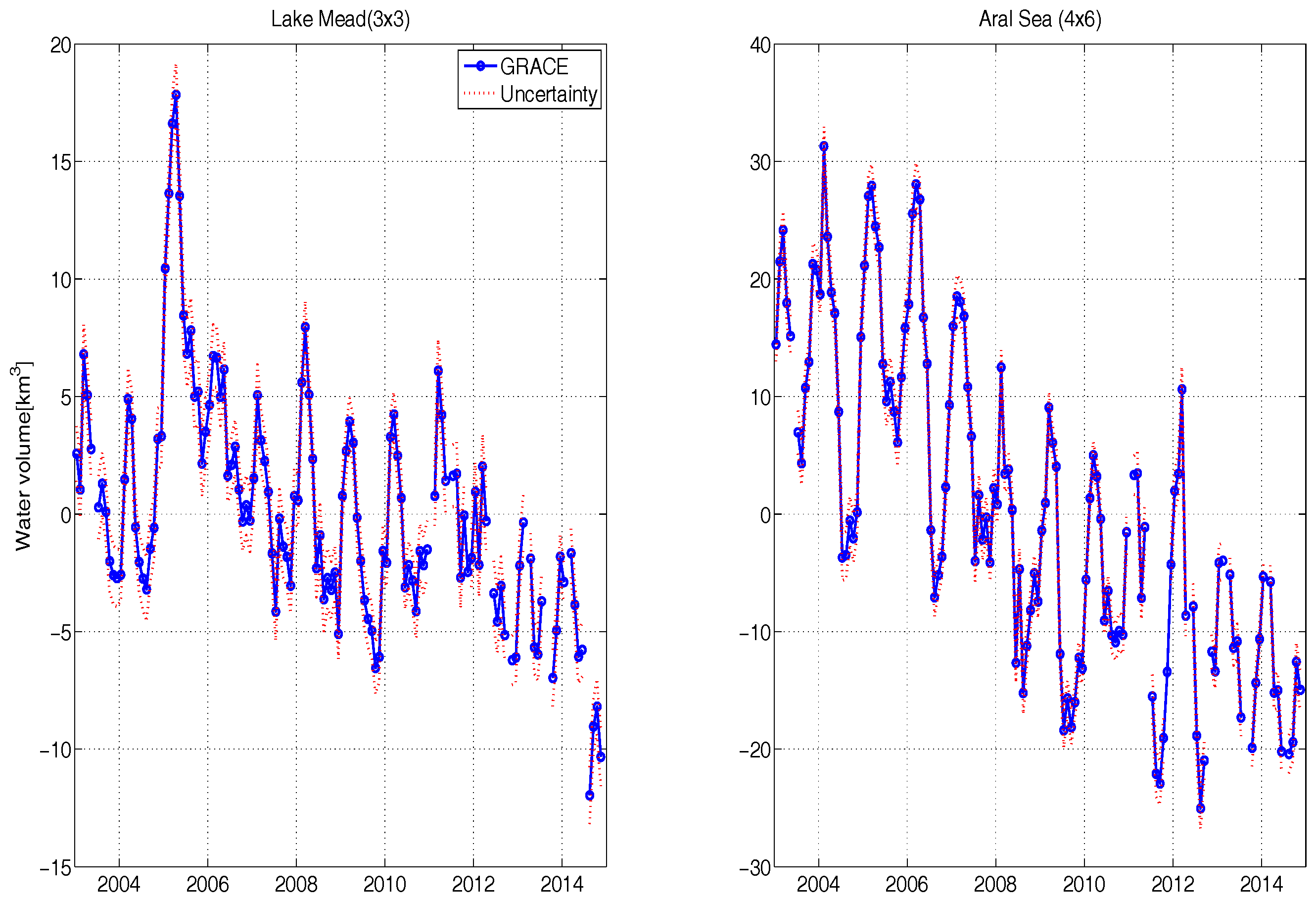
  • Estimation of total water storage variability (ΔTWS) from time-variable gravity data observed by GRACE. The ΔTWS considers the contribution from the surface (reservoirs, river-network, snow, and ice) and subsurface (soil moisture and groundwater) storage changes. However, GRACE cannot resolve individual flux contributions to ΔTWS and the interactions among them.
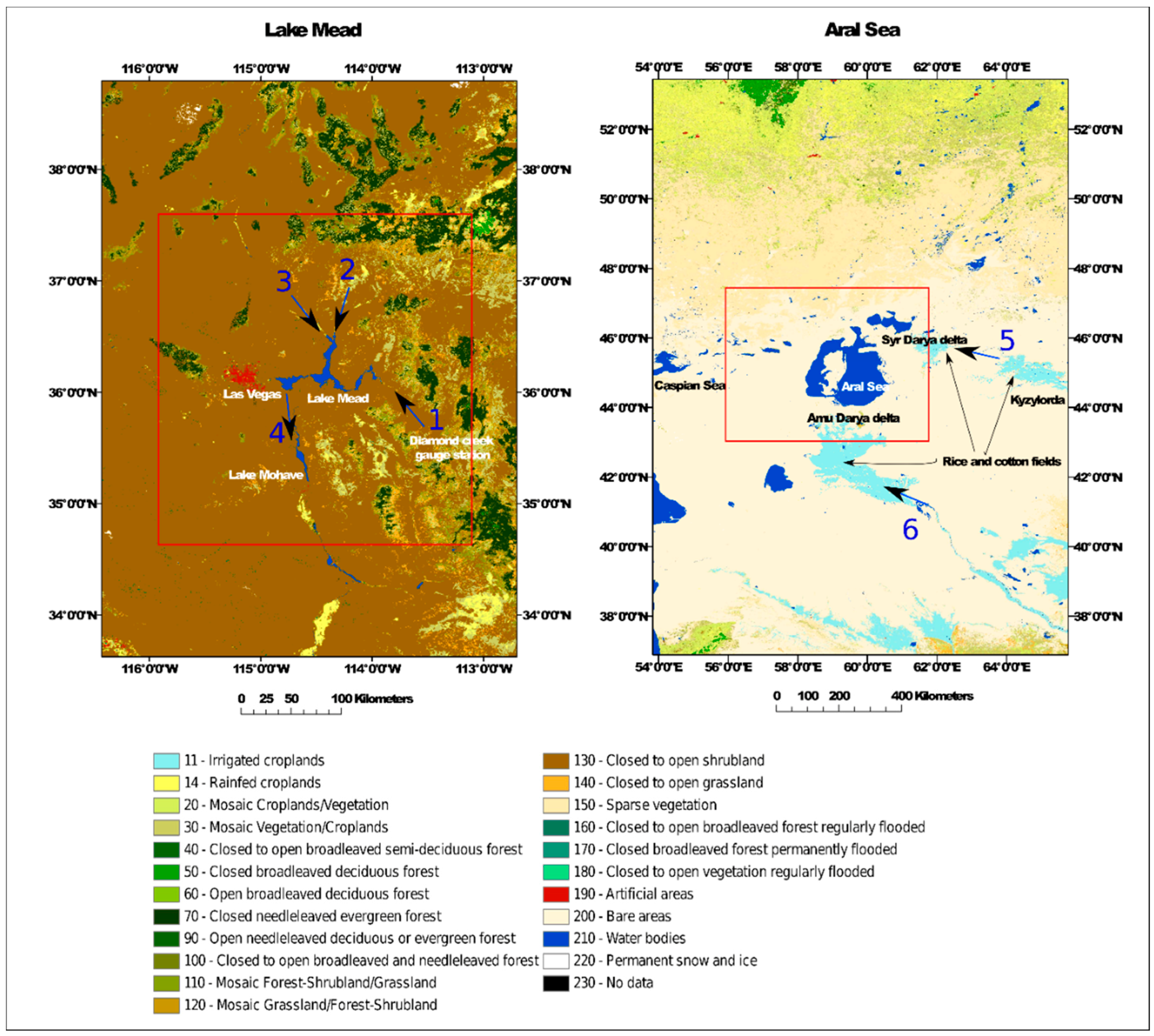
The study analyzes the correlation of ΔTWS from GRACE with the sum of individual fluxes (Equation (1)) as well as with the sum of storages (Equation (2)), in the reservoir-dominated region. The possible inaccuracies caused by different datasets and outputs from different global hydrological models are visualized by comparing two sets of fluxes (discussed in Section 3.1) and two sets of hybrid storages (discussed in Section 3.2). The estimate that best agrees with ΔTWS is considered as the better performer for the region.
Unlike most previous studies, which were conducted at large spatial scales (usually at the basin or global scale) and compared the GRACE signal with hydrological model outputs, this study analyzes the GRACE signal at a small scale by using more accurate storage computations based on the hybrid approach. In few of the previous studies, the GRACE signal was also compared with the combination of storages; for example, Famiglietti et al. [7,8] combined in-situ surface storages with other datasets, de Paiva et al. [8,9,10] combined multiple remote sensing data and model outputs at a larger scale but the spatial resolution of the surface water bodies was 250 m. This study investigates the impact of reservoir variability on the GRACE signal at a small scale and validates the reservoir volume variability estimated at 30 m spatial resolution from remote sensing methods [11].

2. Study Area

This study estimates the hydrological budget of two reservoir regions the Aral Sea and Lake Mead during the period of January 2003–December 2014. The Aral Sea has become a major ecological disaster during the 20th century, due to large-scale irrigation abstraction for rice and cotton fields in central Asia. In comparison, Lake Mead has been declining badly for the past more than a one-and-a-half decade. However, in this case, it is predominantly because of the reoccurring drought since 2000 [12,13]. Lake Mead is the largest reservoir in the United States, formed after the creation of Hoover Dam on the Colorado River. Lake Mead has a comprehensive network of ground observations to validate the space-borne estimates, whereas the Aral Sea has limited means for evaluation. Due to constraints in the spatial resolution of GRACE, a study area larger than the size of the reservoir is selected (Figure 1) (discussed in Section 3.3).
Figure 1 shows the geographic location of the two test sites. The study area is shown in the red rectangular box. The Aral Sea region is approx. 210,000 km2 covering (43° to 47°N) and (56° to 62°E). The Lake Mead region is approx. 90,000 km2 covering (34.5° to 37.5°N) and (116° to 113°W). The land cover map is taken from “GlobCover2009” [14] to analyze the impact of interfering GRACE signal from the surrounding features.

3. Data and Methodology

3.1. Sum of Hydrological Mass Fluxes (ΔS/dt)

Water is continuously exchanged vertically (P and ET) and horizontally (R) between the reservoir and the surrounding land and atmosphere (Equation (1)). Flux-1 is derived by combining ET from WGHM with P from GPCC because WGHM uses GPCC as a climate forcing in the model. While Flux-2 is derived from the combination of ET from GLDAS with P from the TRMM-3B43 product because GLDAS uses a combined product of gauge data and satellite-derived precipitation (discussed in Section 3.2.1). In both of the estimates, the horizontal flux, i.e., surface runoff is obtained from in-situ observations.

3.1.1. Net Surface Runoff (ΔR)

Reservoirs are mostly fed by rivers and normally allow water outflow to ultimately end up in an ocean (e.g., Lake Mead). The Lake Mead study region is mainly fed by the Colorado River, for which we use the Diamond Creek gauge station near Peach Springs (35.77361°N and 113.36278°W) as the inflow into the region and the Davis Dam release (35.19876°N and 114.56949°W) as the outflow from the region (Figure 2 left). These datasets are collected from the annual ‘Water Accounting Reports’ of the United States Bureau of Reclamation (USBR). The other two minor streams, i.e., the Virgin River and the Muddy River (arrows 2 and 3 in Figure 1 left) have a negligible contribution and there are no ground observations at their locations. Therefore, they have been neglected in the calculations. On contrary, endorheic water bodies are terminal lakes with no outflow (e.g., the Aral Sea). The Aral Sea, acts as a terminal point for the two major river basins of central Asia, the Syr Darya in the north and the Amu Darya in the south. The stream inflow and precipitation may only leave out of the Aral Sea by evaporation and seepage. For this study, the Aral Sea river discharge is downloaded from [15]. The data is limited to June 2011, and the exact locations of the gauge stations are unknown.

3.1.2. Precipitation (P)

Precipitation is the main input and evapotranspiration is the main output of water from the atmosphere within a catchment. The Aral Sea region has very sparse rain gauge stations; consequently, the interpolated GPCC data may be relatively less reliable. However, WGHM uses only GPCC rainfall data as a climate forcing for its simulations. Therefore, GPCC precipitation and WGHM ET are combined to estimate the net vertical flux in Flux-1. In contrast, GLDAS uses a combination of NOAA/GDAS atmospheric analysis fields and 2.5° grid Climate Prediction Center Merged Analysis of Precipitation (CMAP), which is derived from blending of gauge data and satellite-derived precipitation and downward radiation observations [16]. Therefore, we apply a comparable TRMM 3B43 (V7) precipitation data, at 0.25° spatial resolution, with GLDAS ET for the net vertical flux estimation in Flux-2. TRMM precipitation product is also used to estimate fluxes over the Lake Mead reservoir (water body only, discussed in Section 4.1).
The dedicated precipitation satellite “TRMM” was launched in November 1997 and turned off in April 2015. The monthly TRMM (3B43) product at 0.25° spatial resolution is obtained from [17]. TRMM (3B43) is a combination of the four independent precipitation measurements, which include the monthly averaged TRMM Microwave Imager (TMI) estimate, the monthly averaged Special Sensor Microwave/Imager (SSM/I) estimate, the adjusted merged-infrared (IR) estimate , and the monthly accumulated GPCC rain gauge analysis [18].
We compare the rain gauge-based GPCC data with the remote sensing-based TRMM product, which combines multiple datasets (Figure 3). The GPCC data comprise monthly mean millimeter level water height and the TRMM data are the hourly precipitation rate, which is multiplied by the number of hours of the respective month to yield monthly precipitation. The monthly precipitation volume is estimated by integrating millimeter-level water height over the study area (4° × 6° for the Aral Sea region and 3° × 3° area for the Lake Mead region). The resulting TRMM and GPCC data are compared in Figure 3, which shows better agreement for the Lake Mead region than the Aral Sea region.

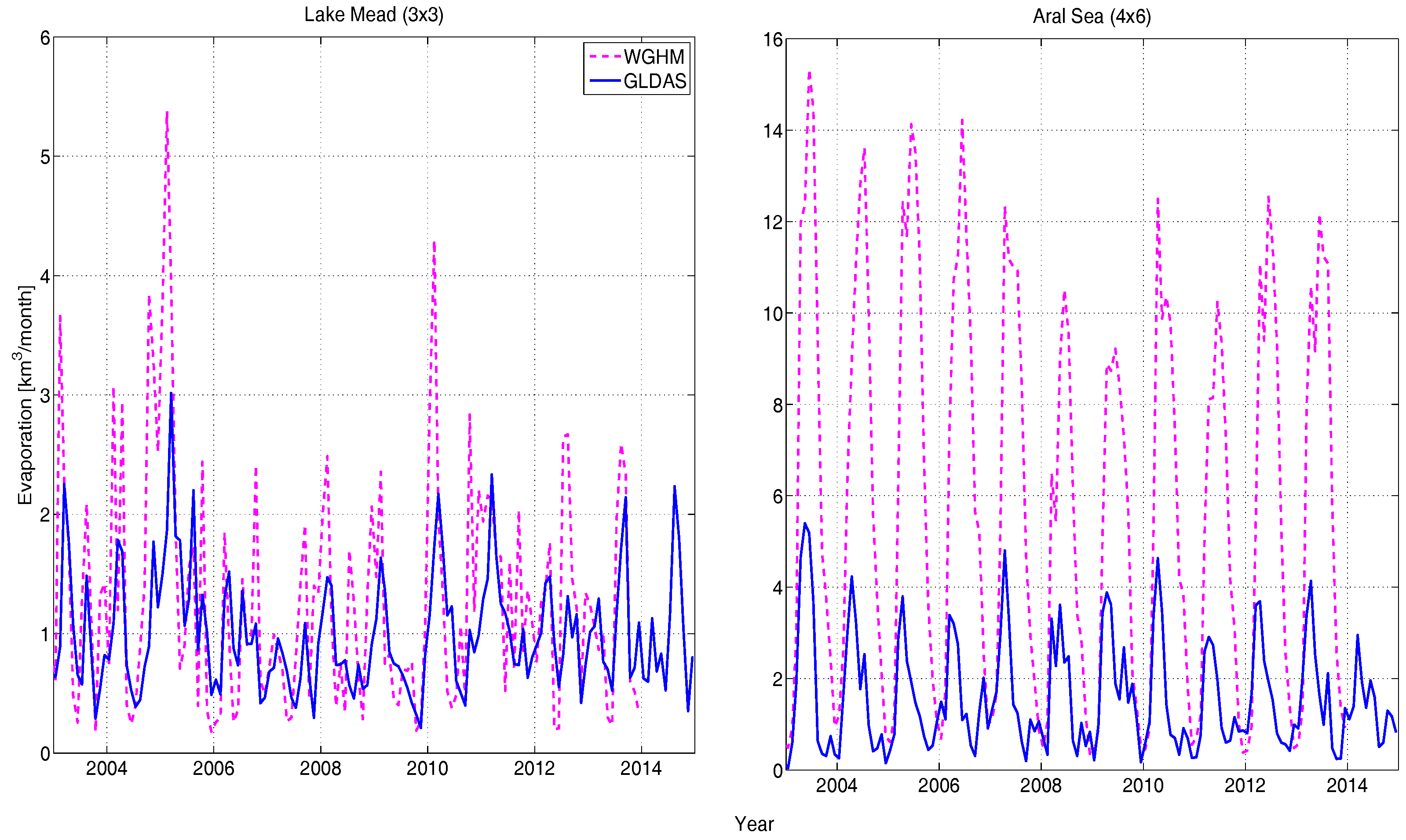
3.1.3. Evapotranspiration (ET)

The rate of ET within a region greatly depends on the amount of water present and the available energy. ET includes evaporation of surface water and transfer of soil moisture by plants through foliage (i.e., transpiration). In arid climates, there is often plenty of available energy to drive ET, but the actual amount of ET varies with the presence of water at the surface, which varies with the change in the reservoir size and availability of upper-layer soil moisture. To derive the total ET of the study area, we use the model output from two global hydrological models: GLDAS and WGHM.
The Noah GLDAS 0.25° data product provides ET at an hourly rate per square meter [16], which is converted to volume per month by multiplying the number of hours in the respective month and the area under study. The WGHM data are based on the Priestley and Taylor equation [19] and are provided in monthly water equivalents (i.e., mm/0.5° grid) as a mean monthly value. The GLDAS data consider the Aral Sea as an ocean and masked it out based on its 1960’s size. Consequently, the ET estimation is very low compared to WGHM (Figure 4 right). However, WGHM also does not explicitly consider the variable surface area of lakes/reservoirs for ET calculation. It includes an empirical and global reduction function that reduces evaporation if the lake storage volume decreases [20]. As this function is not specifically adjusted for the Aral Sea, it may not adequately capture the huge reduction of its water surface area which may be the reason for an overestimation of ET for the region. Furthermore, according to previous studies, the evaporation over the Aral Sea is estimated to be around 1 m to 1.2 m/year [21,22,23], while WGHM estimated it to be much larger for the selected region. Nevertheless, the net flux for the Aral Sea region is only calculated from WGHM (as Flux-1) even with some expected overestimation, whereas outputs from both models are used and compared for the Lake Mead region.

3.2. Sum of Hydrological Storage Compartments (ΔS)

Two hybrid-storage estimates are derived from the combination of outputs from hydrological models with the remote sensing based reservoir volume estimates. The study is confined to reservoir regions; therefore, the respective reservoir is the main liquid surface water body. Its volume is combined with SM and SWE derived from WGHM and GLDAS to generate Storage-1, and Storage-2 respectively.

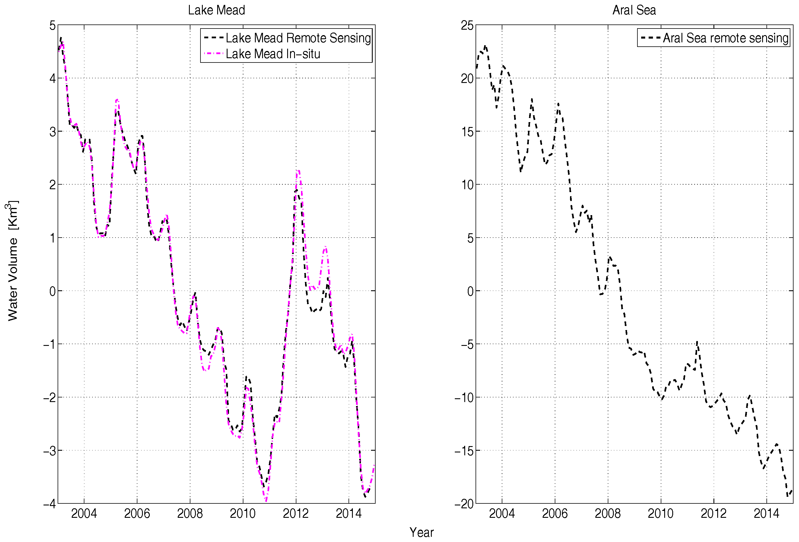
3.2.1. Liquid Surface Water (ΔSW)

We apply reservoir volume estimates using a combination of Landsat, satellite altimetry and bathymetry data for the Aral Sea and Lake Mead, as outlined in our previous study [11]. Figure 5 shows the mean reduced volumetric variations in the two water bodies estimated by the aforementioned remote sensing approach. In our study regions, reservoirs act as major surface water storage components. Figure 5 left compares the remote sensing-based reservoir volume estimate with the in-situ measurements for Lake Mead, which is diligently monitored by the United States Bureau of Reclamation (USBR). However, the Aral Sea has been poorly monitored over the last few decades. Therefore, no ground-based volume estimates are available to validate our previous results [11].

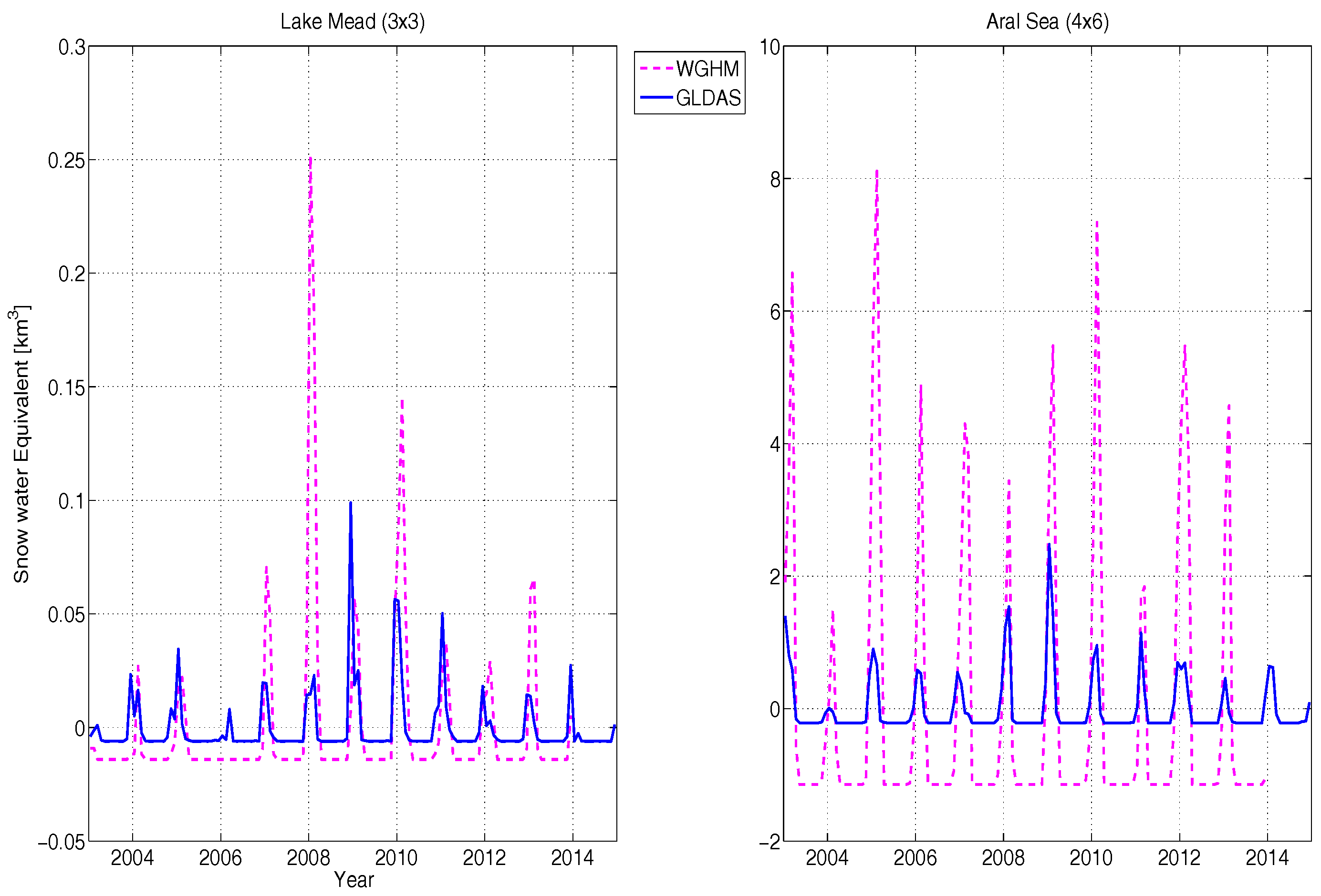
3.2.2. Snow Water Equivalent (ΔSWE)

Apart from rivers and reservoirs, snow and ice are important storage units of surface water, especially for regions in higher latitudes and with large mountain ranges, and have a significant impact on the hydrology of many river systems [21,22]. However, Lake Mead is entirely free of snow and ice; nonetheless, it is fed by snow and glaciers from the Rocky Mountain. The Lake Mead study area contains some mountain ranges. Therefore, little SWE is estimated by both GLDAS and WGHM (Figure 6 left). Conversely, the Aral Sea has three to four months of snow and ice coverage, which is obtained from the two hydrological models. Again, one of the reasons for the underestimation of the SWE by GLDAS for the Aral Sea region is the removal of data from the former extent of the Aral Sea water body (Figure 6 right).

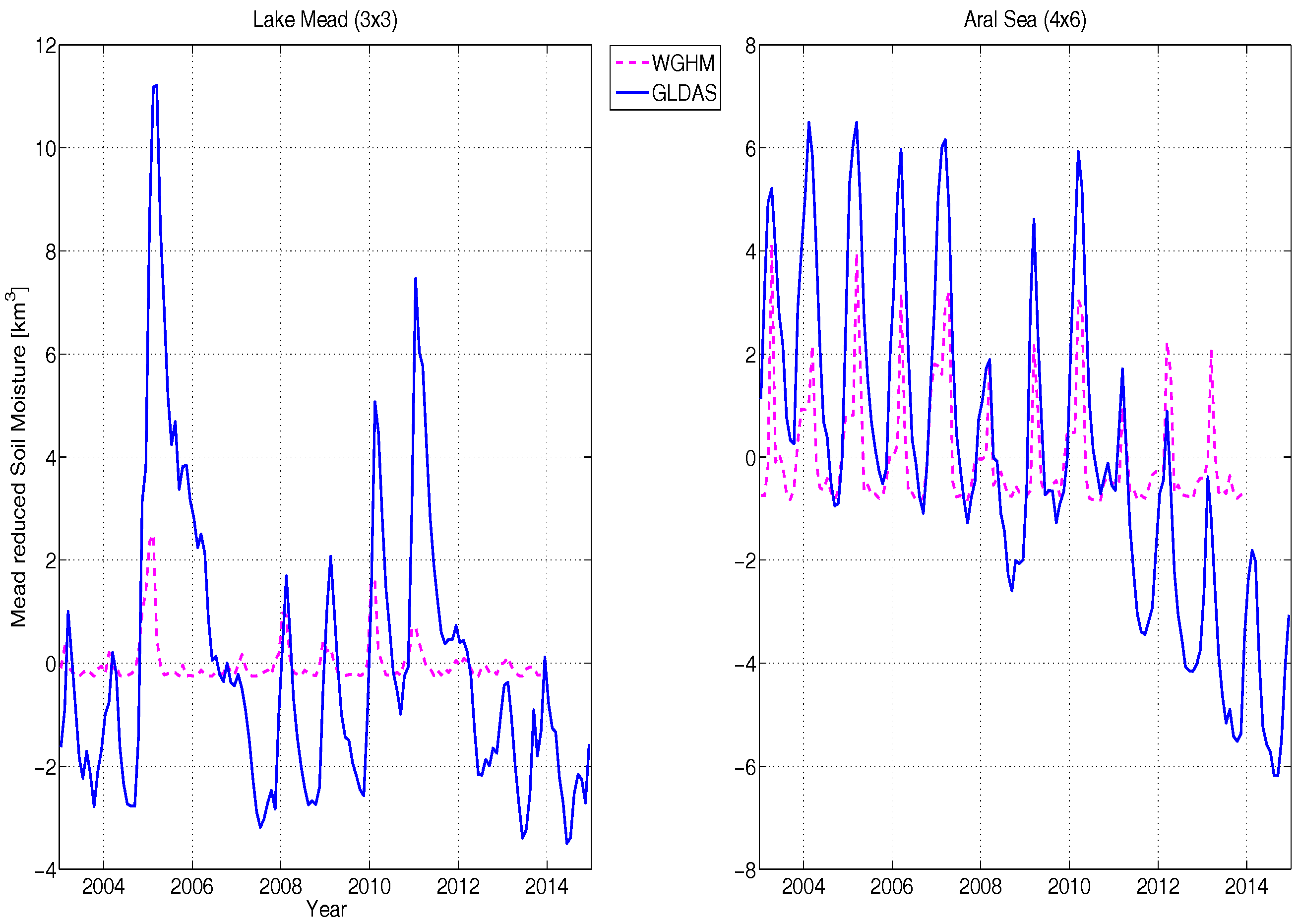
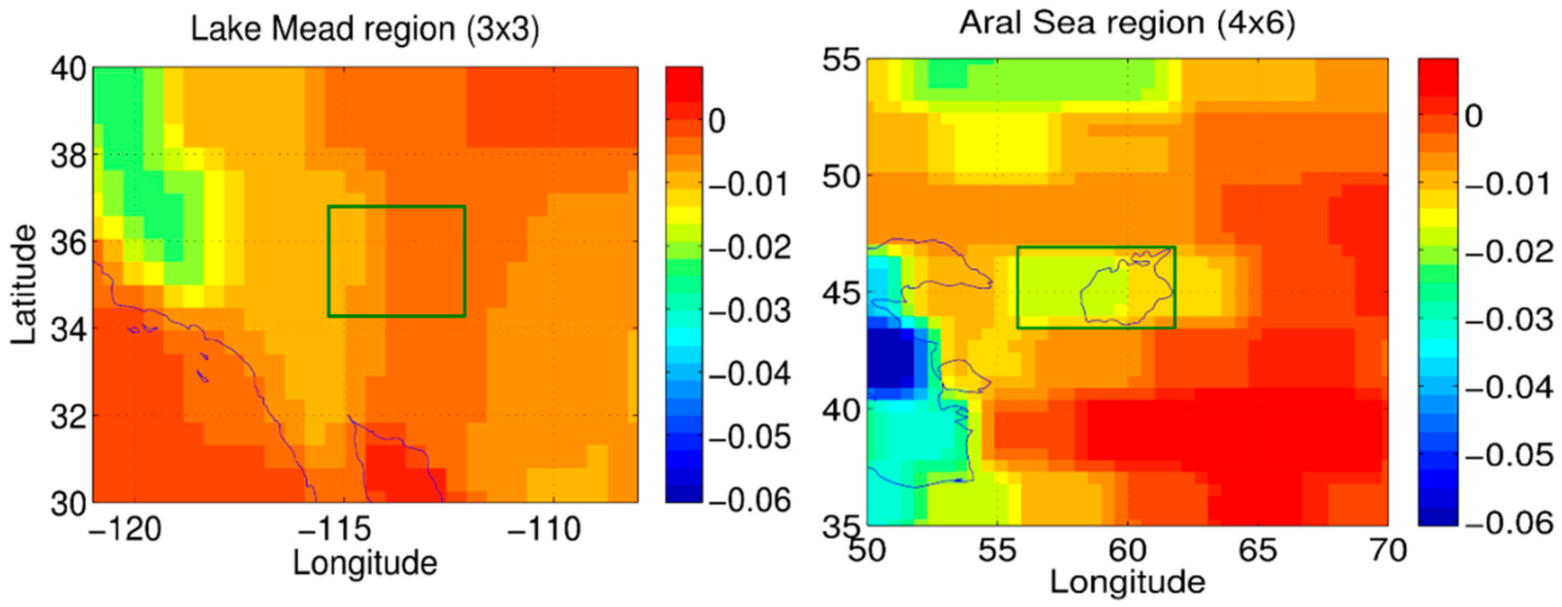
3.2.3. Soil Moisture (Δ SM)

Volumetric soil water content is normally expressed in percentage or volume of water in a volume of soil sample m3/m3. From the Noah GLDAS, we apply the sum of its four soil moisture layers (0–2 m depth), whereas WGHM represents SM for the complete soil profile in a single layer whose depth refers to the rooting depth of the vegetation cover. The mean reduced curves of soil moisture variability estimated by the two models are plotted in Figure 7. WGHM features lower amplitudes for both regions, even though the Aral Sea is again largely masked out in GLDAS.
The SM estimates by GLDAS in 40–100 cm and 100–200 cm root depth have higher and smooth variations during the study period. However, after 2010 flood in the Aral Sea region, it experienced a marked decline in the GLDAS simulations for which the reasons are unknown at this point. As mentioned before, WGHM considers soil moisture for the root zone, of which the depth is determined as a function of the actual land cover. For the Aral Sea, much of the surroundings is classified as bare soil (root depth 0.1 m in the model), with smaller fractions of open shrub land (0.5 m) or grassland (1.0 m). Thus, the overall storage capacity of the soil in WGHM for this region is small which results in low storage values and low storage variations. The same applies for the Lake Mead region, which is predominantly classified as open shrub land in WGHM.

3.3. GRACE-Derived ΔTWS

For over 14 years, the time-variable gravity field solutions computed from GRACE data have enabled to study the total mass change at regional and global scales [24,25,26,27]. GRACE has also been used for comparisons, validation and calibration of hydrological models [28,29,30]. The ΔTWS from GRACE was compared with in-situ observations [31,32,33], altimetry observations [32,34,35,36] and hydrological models [36,37,38].
To determine the monthly GRACE-derived water mass variability in the study area, the JPL mascon solutions [39] are evaluated. In contrast to the more common way of parameterizing the gravity field in terms of global spherical harmonic basis functions, the mascon representation is based on local equal-area three-degree spherical cap mass concentration blocks (mascons). During the gravity field estimation process, monthly scaling coefficients are estimated for each of these mascons to represent the global mass distribution. The mascon representation allows a straightforward way to introduce both spatial and temporal constraints between individual basis functions into the GRACE data processing. These constrains allow to filter out the noise which is present in the GRACE satellite data, and which has led to a typical north-south error stripe pattern in the unconstrained monthly gravity field solutions based on spherical harmonics. While for the spherical harmonic solutions these error patterns have to be removed in a dedicated post-processing filtering step (de-striping), no post-processing filtering is necessary for the mascon solutions. However, while the constraints applied in the estimation process reduce the noise, they also result in a damping of the signal and in a coarse spatial resolution, causing a signal to be spread out over a larger area than the area which it originates from (leakage effect). This signal damping can be counteracted by applying so-called rescaling coefficients [40] to the gridded water storage changes, which are determined from a comparison of unfiltered vs. smoothed hydrological model output and which are provided on the GRACE Tellus website for download [41].
We use the mascon solutions in the version which applies the Coastline Resolution Improvement (CRI) filter, for more information see [39]. The GRACE solutions were corrected for geocentric motion coefficients, according to [42] and for variations in Earth’s oblateness (C20 coefficient) obtained from Satellite Laser Ranging [43]. The Glacial isostatic adjustment has been accounted for using the model by [44]. The uncertainty data is downloaded from the Tellus website at a 0.5-degree grid and represents the uncertainty of each mascon estimate. These uncertainty measures are derived from the formal covariance matrix of the mascon solutions, scaled differently over oceanic and continental areas in order to obtain more realistic error bounds that match, e.g., the errors known from a comparison between GRACE and ocean bottom pressure data.
The size of the study boxes is chosen such, that it can be resolved by GRACE and―at the same time―that hydrological mass variations in the vicinity of the reservoirs influence the GRACE measurements as little as possible. The Lake Mead study box is based on the size of the mascon (3° × 3°). Lake Mead is a small reservoir (approx. 430 km2 area and 27.5 km3 volume in spring 2003) and resembles a point mass at the center and the study area, which is approx. 200 times larger than the reservoir area (Figure 8 left). The position of the point mass (reservoir) strongly affects the GRACE signal [45]; therefore, the study area is selected around the reservoir mass center. The Aral Sea surface area was approx. 20,000 km2 in spring 2003 (with 92.5 km3 volume). Hence, it requires data from more than two mascons to cover the entire Aral Sea (Figure 8 right). The study area is extended towards the west of the Aral Sea in order to include the entire signal of the Aral Sea mass change from which we assume that it is smoothed over the complete western mascon. In 2003, the Aral Sea was approx. one-tenth of the size of the selected study box. In Figure 8, the twelve years (January 2003–December 2014) mascon GRACE solution shows a negative trend in the equivalent water height (EWH in meter/year) of the selected study regions.
The derived mass variations for the two regions are shown in Figure 9. The uncertainty range (red dotted line) is retrieved from GRACE Tellus on a 0.5-degree grid. It represents the uncertainty of each mascon estimate, except for November 2011. There are few data gaps in the GRACE data, especially since 2011 due to the aging batteries of the satellites. During certain orbit periods over 4–5 consecutive weeks, no ranging data are collected and hence no gravity fields can be computed approximately every 5–6 months [46].

4. Results

4.1. Lake Mead (Reservoir) Water Budget

Lake Mead is mainly fed by the Colorado River and its discharge budget is summarized in Equation (3) (Figure 1 left). The overall discharge and peak flows of the Colorado River to Lake Mead at Glen Canyon (Lake Powell) and from Lake Mead at Hoover Dam are highly regulated.
Lake Mead discharge budget = Colorado River inflow (Peach Spring gauge station) + Muddy River and Virgin River + LV Wash − Hoover Outflow − Lake Mead recreational diversions
The Hoover Dam release and Lake Mead diversions for recreational purposes are derived from the annual “Water Accounting Reports” of the USBR [47]. Las Vegas Wash return inflow is obtained from the USGS surface water database [48]. The inflow at the north arm of Lake Mead from the Muddy River and Virgin River is not directly measured by the USBR and other agencies and therefore is not considered in the calculations. The top panel of Figure 10, shows the Lake Mead discharge budget. The bottom panel of Figure 10 compares the derivatives of the reservoir volume (computed by single differences) obtained from remote sensing and in-situ measurements (Figure 5 left) with the sum of water fluxes acting on the reservoir.
The net fluxes acting on approx. 450 km2 area of the reservoir is obtained by reducing the net discharge budget by the vertical flux acting over the water body and the leakage to the bank storage Equation (4):
∆Mead storage = Lake Mead discharge (total inflow − Hoover outflow) + Precipitation on the reservoir − Lake Mead Evaporation (in-situ) − ∆Mead Bank storage
Monthly time series of evaporation (only from the Lake Mead water body) are obtained from personal contacts from the Boulder Canyon Operations Office. The estimated evaporation is obtained by multiplying a monthly coefficient (derived from studies conducted by the USGS) by the average of the surface area of previous and current months. Precipitation over the reservoir is obtained from the TRMM (3B43) data. The Mead bank storage is a volumetric representation of shallow groundwater levels immediately adjacent to a reservoir. The amount of bank storage is not subject to an exact determination. However, such storage typically fills voids within nearly 5 km of the reservoir [49]. The Mead bank storage fluctuates with changes in the reservoir storage. Therefore, the bank storage is estimated by multiplying the change in reservoir storage by a coefficient of 0.065, provided by the USBR.
Furthermore, we interpret the GRACE signal in the reservoir region. As GRACE cannot observe just the small reservoir, therefore, a 3° × 3° window around the reservoir is analyzed.

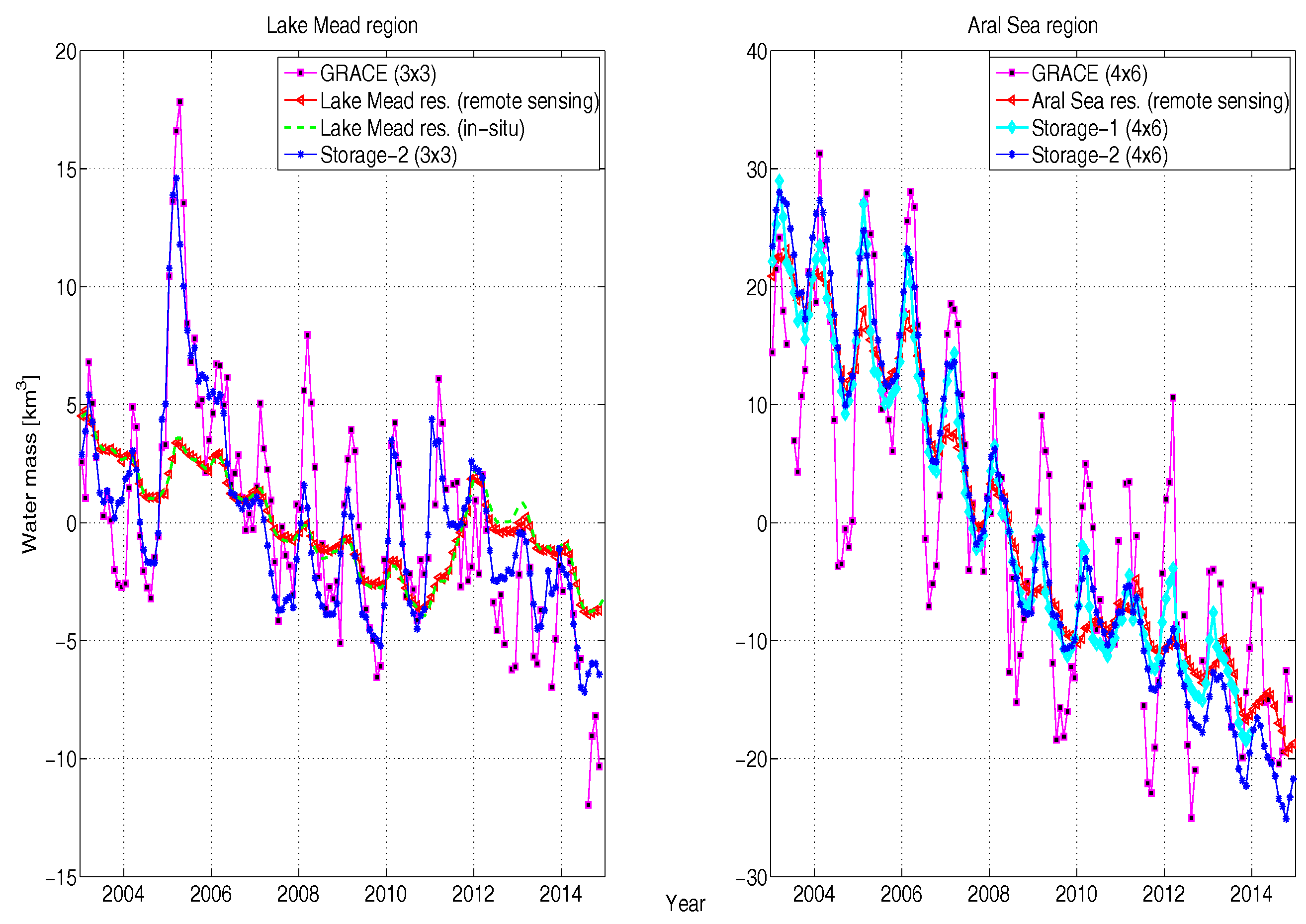
4.2. Lake Mead Region (3° × 3°) Water Budget

In Figure 11 (top), the sum of the fluxes (Flux-1 and Flux-2) is compared with the derivatives of the hybrid-storages (Storage-1 and Storage-2) and ΔTWS from GRACE. In the bottom panel of Figure 11, the fluxes are reduced by their seasonality (i.e., a mean value of each January, February, etc., over the study period) and then integrated to obtain the inter-annual variability. Furthermore, each time series are mean reduced, to compare with each other. Similarly, the hybrid-storages and the ΔTWS GRACE are reduced by their seasonality (Figure 11 bottom). In addition, all the time series in Figure 11 are smoothed by applying a three-month moving average window to derive their gentle progression. The derivative plot (Figure 11 top) shows the variations two to three months in advance of the integral plot (Figure 11 bottom) because the prior captures changes in the trend; for example, a decrease in precipitation will suppress the rate of increase, however, it is still filling the storages. Furthermore, the bottom plot has only non-seasonal anomalies.
This region normally receives maximum water by winter rains and spring runoff from snow and glacier melts. During the study period, the lower Colorado region underwent recurring drought [50], except between 2004 and 2005, when it experienced exceptional rain (Figure 3 left), whereas the 2011 gain in Figure 11 is mainly driven by exceptional upstream runoff.
The mass evolution and its different phases are analyzed below to understand the driving force and differences in the estimations. The periods to be discussed are shown as the large numbers at the top of Figure 11.
Period-1 (March 2003–September 2004): All datasets observed a slight loss (0.6–1.6 km3 /year) of the water mass.
Period-2 (October 2004–May 2005): Heavy rain escalated the GRACE signal and Storage-2 for more than 13 km3 within seven months (Figure 3 left). However, Storage-1 increased much less, because it is mainly driven by the reservoir trend, as soil moisture is highly underestimated by WGHM for this region (Figure 7 right). Similarly, Flux-1 increased less than 5 km3 and Flux-2 jumped 22 km3. The difference can mainly be attributed to the difference in ET between WGHM and GLDAS (Figure 4 right) and in precipitation from GPCC and TRMM (Figure 3 left) for this period. This shows high uncertainty in the estimation of fluxes and storages depending upon the input datasets. The reservoir itself had less gain during this period as it received regular input from upstream, but at the same time, it had relatively less outflow for a few months (Figure 2 left).
Period-3 (June 2005–April 2006): Due to the higher moisture availability in the soil during the previous period, the ET rate increased (Figure 4 left) in the follow-up period. GRACE and Storage-2 lost more than 10 km3 within 10 months. Storage-1 also exhibited losses similar to the reservoir (approx. 3 km3) due to the underestimation of SM by WGHM (Figure 7 right). This shows that possibly during the period 2 and 3, soil moisture variability might be the strongest contributor among the different storage compartments of the GRACE data.
Period-4 (May 2006–December 2009): GRACE observed a similar low mass loss rate as other datasets. The 2008 winter anomaly was due to added input from precipitation (Figure 3 left). The continuous runoff deficit (Figure 2 left) caused by extra withdrawal from the reservoir to cater lower basin demands and possibly a decline in the ground water table is a cause of this slow and continuous mass decline.
Period-5 (January 2010–December 2010): A slight gain is observed by four of the datasets, except by the reservoir and Storage-1. This may be due to above-average rainfall in January, October and December 2010 (Figure 3 left). However, reservoir volume and Storage-1 continued to decline because of no change in the runoff pattern (Figure 2 left).
Period-6 (January 2011–December 2011): Additional heavy input from the upper Colorado basin increased the reservoir volume during this period. All datasets exhibit an increase in volume. In contrast to the Period-2 mass gain, which is caused by precipitation in the study region, the increase during Period-6 is caused by inflow from upstream areas. This suggests that this period might be dominated by the reservoir trend (Figure 5 left).
Period-7 (January 2012–December 2014): Most of the increase in water from the previous period is lost again within six months, followed by continuous mass loss over the final three years of the study period at more than 1 km3 per annum. During this persistent drought with abnormally low snow in the Rocky Mountains [50] and low rainfall in the region (Figure 3 left), GRACE exhibited greater mass loss than Storage-2, which might indicate significant ground water extraction.
Among all the applied datasets in the Lake Mead region, the GRACE signal agrees best with Storage-2 (GLDAS based estimate) (Figure 11). In Storage-1, WGHM highly underestimates the SM for these regions (as discussed in Section 3.2.3). Reservoir volume is the only major contributor to Storage-1 estimate. Therefore, in Figure 11 the Storage-1 and reservoir volume plots are overlapping. Among the fluxes, Flux-2 show a better correspondence to ΔTWS, even though, it occasionally tends to overestimate of the variability. In period-2, Flux-1 (Figure 11 top) underestimates ΔS/dt compared to ΔTWS while Flux-2 overestimates it. This can be explained by the difference between P from GPCC and TRMM (Section 3.1.2) and the ET simulation by WGHM and GLDAS (Section 3.1.3) respectively.

4.3. Aral Sea Region (4° × 6°) Water Budget

In the Aral Sea region, the entire hydrological characteristics have been modified since the lake is undergoing a drastic decline. Further, unlike Lake Mead, the Aral Sea region has limited data availability. There is almost no monthly ground observation for its volume and the applied runoff data are provided without exact coordinates and only for a limited duration. Also, the hydrological models have limited applicability in this region. GLDAS data have flagged the 1960’s size Aral Sea area as an Ocean and masked it out, i.e., the model does not perform any simulations for this area. The maximum effect of not including the Aral Sea surface water in the model input becomes apparent in ET estimation. ET is mainly driven by the availability of water and temperature and neglecting such a vast water body in the model input, has a serious impact on the ET estimates (Figure 4 right). Therefore, we do not compute Flux-2. Similar to the Lake Mead region, Figure 12 top shows derivatives of the mass variation from GRACE, hybrid storages (Storage-1 and Storage-2) and the Aral Sea volume as well as the time series of the sum of the hydrological fluxes (Flux-1, i.e., P (GPCC) − ET (WGHM) + ΔR (in-situ)). The lower panel shows the mean reduced integrated non-seasonal variations.
The detail hydrological mass evolution of the Aral Sea region is given below.
Period-1 (March 2003–December 2003): In the first year of the study period a slight increase is observed in the lake volume resulting from some extra drainage from the Amu Darya (Figure 2 right). In contrast, GRACE and Flux-1 increased significantly because of the additional contribution from the above-average rainfall (Figure 3 right).
Period-2 (January 2003–April 2006): This period experienced a relatively low rate of decline (2–3 km3/year) in the water mass. However, Flux-1 does not agree well with the results of other approaches.
Period-3 (May 2006–February 2010): A staggering decline was observed by GRACE and Storage-2 in this period; water mass decreased at approximately 7 km3 per annum. The Aral Sea lake and Storage-1 also receded at a rate of 6 km3 per annum. This period was dominated by the upstream cut off of the drainage [51], and subsequently, driven by the lake trend.
Period-4 (March 2010–September 2010): Within less than half a year, GRACE observed more than 9 km3 non-seasonal gain. The region experienced above-average rainfall (Figure 3 right), followed by an increase in the lake volume (more than 4 km3) due to heavy upstream runoff (Figure 2 right). The increase in GRACE mass signal during this period is contributed not only by the Aral Sea lake gain but possibly also by storages in the Aral Sea delta, surrounding small lakes, irrigated croplands and increase in soil moisture.
Period-5 (October 2010–April 2011): The region lost most of the volume that was acquired during the previous period, and the lake lost approx. 3 km3 within six months. This decrease is possibly due to large-scale evaporation resulting from an increased water surface area in the Aral Sea and its surrounding storages, as well as moisture in the top layer of the soil.
Period-6 (May 2011–November 2014): Due to sporadic rain, GRACE observed relatively less decline in the last three and a half years of the study, at about 1.5 km3/year. However, the lake shrunk to its all-time minimum in 2014 by completely losing its southeastern lobe [51,52], which indicates very limited runoff during this period.
For the Aral Sea region, Flux-1 exhibits a different inter-annual signal in the region over the entire study period (Figure 12) and features a huge mass loss between 2005 and 2010. This can be explained by the overestimation of ET by WGHM (discussed in Section 3.1.3) and the underestimation of P by GPCC (discussed in Section 3.1.2). On the contrary, both hybrid-storages show a very good agreement with the GRACE signal because of the strong contribution of the Aral Sea volume trend. The difference between hybrid storages and ΔTWS from GRACE can be predominantly explained by the underestimation of SM by the hydrological models and the role of surface water storage in the delta region. The ΔTWS also has signals from the Amu Darya and Syr Darya delta and several small lakes in the two deltas, which store a significant part of the inflow from the river.

5. Discussion

The study demonstrated that the estimated reservoir flux agrees very well with the remote sensing-based Lake Mead volumetric variation (Figure 5 left), showing 90% correlation with the in-situ and 81% with the remote sensing-based estimates (Figure 10 bottom). Net runoff is the major contributor in the estimated total flux, as seen from Figure 10 bottom. The vertical flux (blue line in Figure 10 bottom) is always negative, which means that evaporative loss from the reservoir is greater than precipitation, and the sum is significantly less in the total flux (green line in Figure 10 bottom). The RMSE (root mean square error) between the estimated total flux and the remote sensing-based storage variation is 0.22 km3, which can be attributed mainly to the errors in volume estimation of the reservoir. Especially when the trend of increasing/decreasing volume changes, the prior overestimations/underestimations by the remote sensing method (Figure 5 left) become more pronounced. Furthermore, the remote sensing estimates are obtained using a combination of two data products (Landsat and altimetry). When data cannot be provided by one of the products, the combined model shifts towards the available data, which can lead to a slight drift in the variability. Furthermore, the difference between the sum of fluxes and the reservoir storage variation is also affected by limitations in the flux estimates. The net flux estimate neglects other minor inflows into Lake Mead due to data unavailability, for example, the contributions from the Virgin River and Muddy River, and the precipitation flowing into the reservoir from the surroundings. In addition, the evaporative loss from the Colorado River, covering approx. 100 km between the Gauge station and the reservoir and the ground water interactions are not considered.
This paper further analyzes the cause of mass variations in the two study regions observed by GRACE during different periods by combining different datasets. The periods of more than average rainfall and increase in net runoff generally coincided with an increase in the GRACE signal. There were periods when GRACE and the water bodies had different signals caused by variation in the amount of precipitation in the region; for example, those in periods 2, 3 and 5 of the Lake Mead region and period-1 of the Aral Sea region. During these periods, it is possible that the variability in SM dominated the mass change. Abelen et al. [53] also emphasized that the SM can strongly contribute to the GRACE signal. Conversely, there are periods dominated entirely by the variability in the water body, e.g., period-6 of the Lake Mead region and period-3 of the Aral Sea region. This detailed analysis of water balance inconsistencies, suggests improvements in the parametrization of a particular hydrological model output should be made; for example, SM and ET estimates in WGHM must be recalculated for the selected regions. It can also help to visualize some possible contribution of other geophysical parameters like ground water, canopy storage, and non-hydrological mass variations, by closing the water budget of a region. Water inflow in arid/semi-arid regions is quite unevenly distributed over time. The water gained by heavy rain/runoff was also quickly lost at both of the test sites, which can be intelligently harnessed if there is a better understanding of the different hydrological contributors in the region.
The results showed that the accuracy of the interpretation of the GRACE signal is limited by errors in the datasets and varies with different datasets/model output combinations, for example, as in Period-2 of the Lake Mead region. The long-term non-seasonal flux estimates have overestimated the mass loss and gain at different periods, due to aggregated uncertainty in the sum of vertical fluxes ( P E T ) and integrated error propagation. There are substantial differences between the amount of accumulated precipitation and their intensities from different precipitation datasets [54,55,56] and ET is one of the most uncertain variables in the global hydrological models [29]. Overestimation of ET leads to an underestimation of potential water mass and vice versa. For example, in the Lake Mead region, most of the above average rainfall (Figure 3 left) during period-2 (2004–2005) is directly removed by higher ET in WGHM contrary to GLDAS (Figure 4 left). Furthermore, SM is underestimated by WGHM due to smaller root zone (discussed in Section 3.2.3). Therefore, Flux-1 and Storage-1 show lower water mass than Flux-2 (not estimated for the Aral Sea region) and Storage-2 for both study regions. This indicates a deficient model structure or parameterization of WGHM for these regions. The uncertainty of the Aral Sea flux estimate is higher because of the significant difference between TRMM and GPCC precipitation data (Figure 3 right), unavailability of gauge location of the runoff and erroneous ET estimation. Using a dynamic mask of water extent over the Aral Sea and applying the evaporation rate calculated by previous studies [21,22,23] might result in better ET estimates here.
Table 1 and Figure 13 compare the ΔTWS observed by GRACE with the mass variations determined by different approaches. Table 1 shows that for the Lake Mead region the fluxes correspond better with the GRACE derivatives at Lag 1, which means a time lag of 1 month. Hence, GRACE data tend to describe the water mass change a month later than the flux estimates. The reason for that is that GRACE observations need to be collected over one month before a mass change can be computed. The fluxes on the other side capture it immediately. The upper panel of Figure 11 shows that the GRACE signal usually lagged behind the net fluxes by 1 month, except for the period-6 peak, which is driven by heavy runoff inflow between late 2009 and early 2010.
The results demonstrate that among all the applied datasets Storage-2 (GLDAS and remote sensing of reservoir volume-based hybrid ΔS) worked well for these regions. However, in the Aral Sea region, both the storages have above 80% correlation with ΔTWS because the reservoir is the major contributor to the GRACE signal. However, the seasonal peaks are significantly underestimated in both hybrid storages because minor contributions also come from the Aral Sea delta, many small adjoining lakes, and other hydrological compartments. The impact of hydrological outputs in the region increases with decreasing lake size (Figure 13 right). In the Aral Sea region, Storage-2 has slightly high RMSE compared to Storage-1 (Table 1) because of the masking of the 1960s lake extent in GLDAS in SM and SWE simulations. Further, in the Aral Sea region, the lake is undergoing huge water mass changes, whereas SM and SWE in the surrounding region feature almost no inter-annual signal (except GLDAS SM after 2010). This indicates anthropogenic forcing and upstream water abstraction. The contribution of SM and SWE compartments in the Lake Mead region is greater than the reservoir, that is why the reservoir trend is only 60% correlated with the GRACE signal. Further, in the Lake Mead region, SM and SW show a mostly similar inter-annual signal, which indicates a uniform water storage change driven by climate forcing.
Due to the very small study area (90,000 km2) of the Lake Mead region compared to the GRACE resolution (200,000 km2 based on satellite orbital height of ~450 km), there is a possibility that the GRACE signal dampens due to leakage to the regions outside the study box. Longuevergne et al. [45] also emphasized that when the basin area is smaller than 300,000 km2 the apparent GRACE signal is underestimated for point masses. However, the signals of mass variability will remain the same, as point mass (Lake Mead) is in the center and there is no other point mass in the surrounding region. In contrast, the study area of the Aral Sea region is much larger and located close to the Caspian Sea, which can contaminate the GRACE signal. However, the mascon-based regional GRACE solution has an improved spatial resolution for this region due to the absence of a de-striping filter.
Accurately closing the water budget of any region is still an open problem. There are regions where the hydrological models fail to represent the hydrological states. For example, WGHM did not perform well in these two regions. Further, there are differences in the estimates of ΔTWS by different GRACE solutions [45]. Therefore, if the actual distribution of water is not evaluated, there can be significant error in the ΔTWS analysis of the GRACE signal. Many previous studies estimated GW storage changes by subtracting GRACE ΔTWS by the sum of other storage compartments derived from model outputs [57,58,59]. However, in this study, the role of ground water storage is neglected because of the non-availability of the data. In the case of Lake Mead, GW can account for the difference in Storage-2 and ΔTWS. For example, Castel et al. (2014) [60] showed declining water levels of many well stations in/around Las Vegas. However in the Aral Sea region, according to Cretaux et al., (2013) [23] the lake has an almost negligible GW contribution. Our study suggests that the combination of remote sensing-based reservoir storage with model outputs can better interpret the mass variations in GRACE, as opposed to the aforementioned entirely hydrological model-based approach. However, this method needs to be tested in more regions and for a larger area and cautious conclusions need to be drawn considering the uncertainties of the different datasets.

6. Conclusions

TWS is the integral physiographic characteristic of any territory, determined by its specific climate features, typical landscapes, and land use. The two test sites in this study are located in arid/semi-arid regions, where water is the most limiting factor for the evolution of life. Lakes/reservoirs are the major contributors of surface water volume in most of the regions. Therefore, authentic knowledge of their characteristics and dynamics is essential for short and long-term water management of a region. The main findings of the study are:
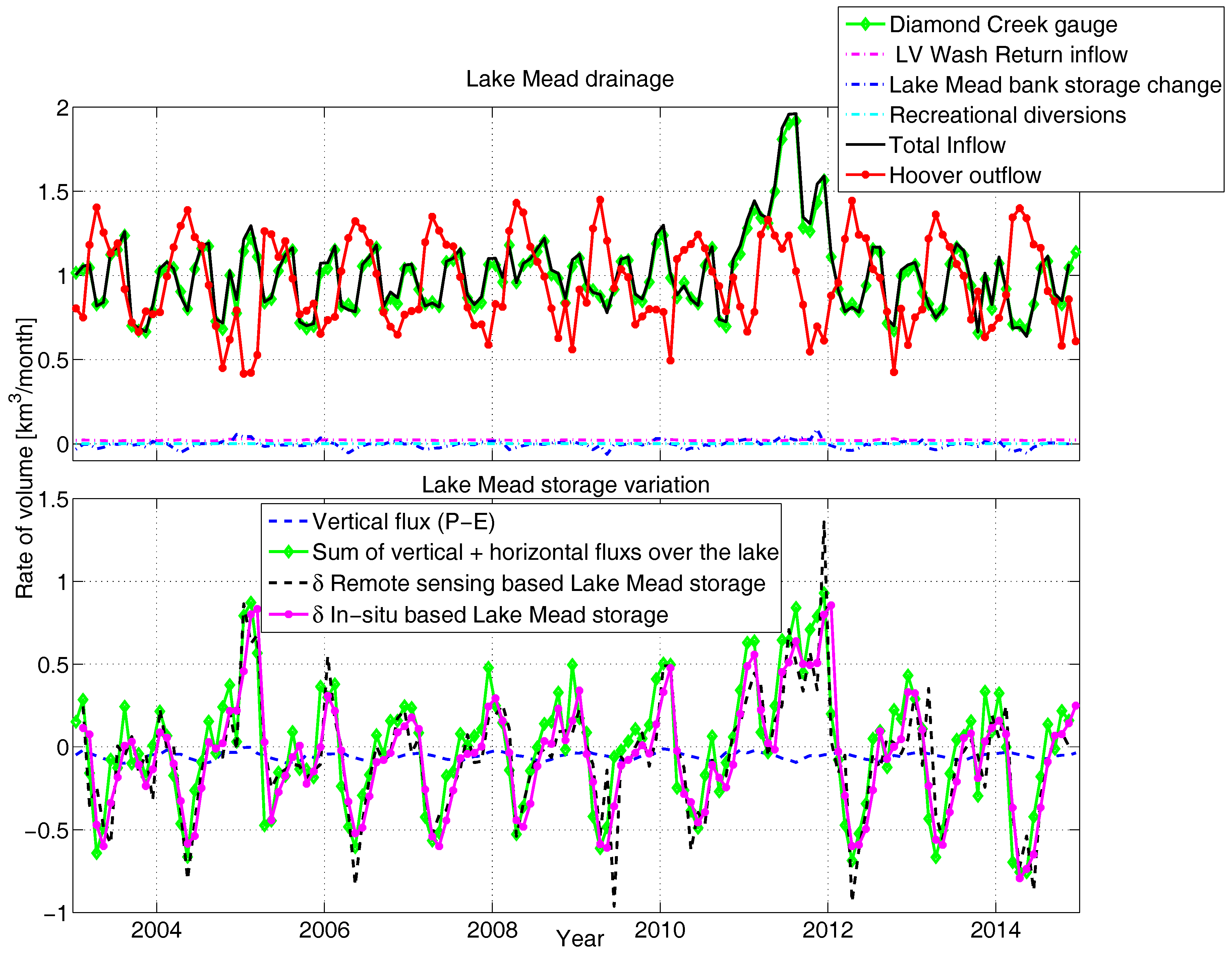
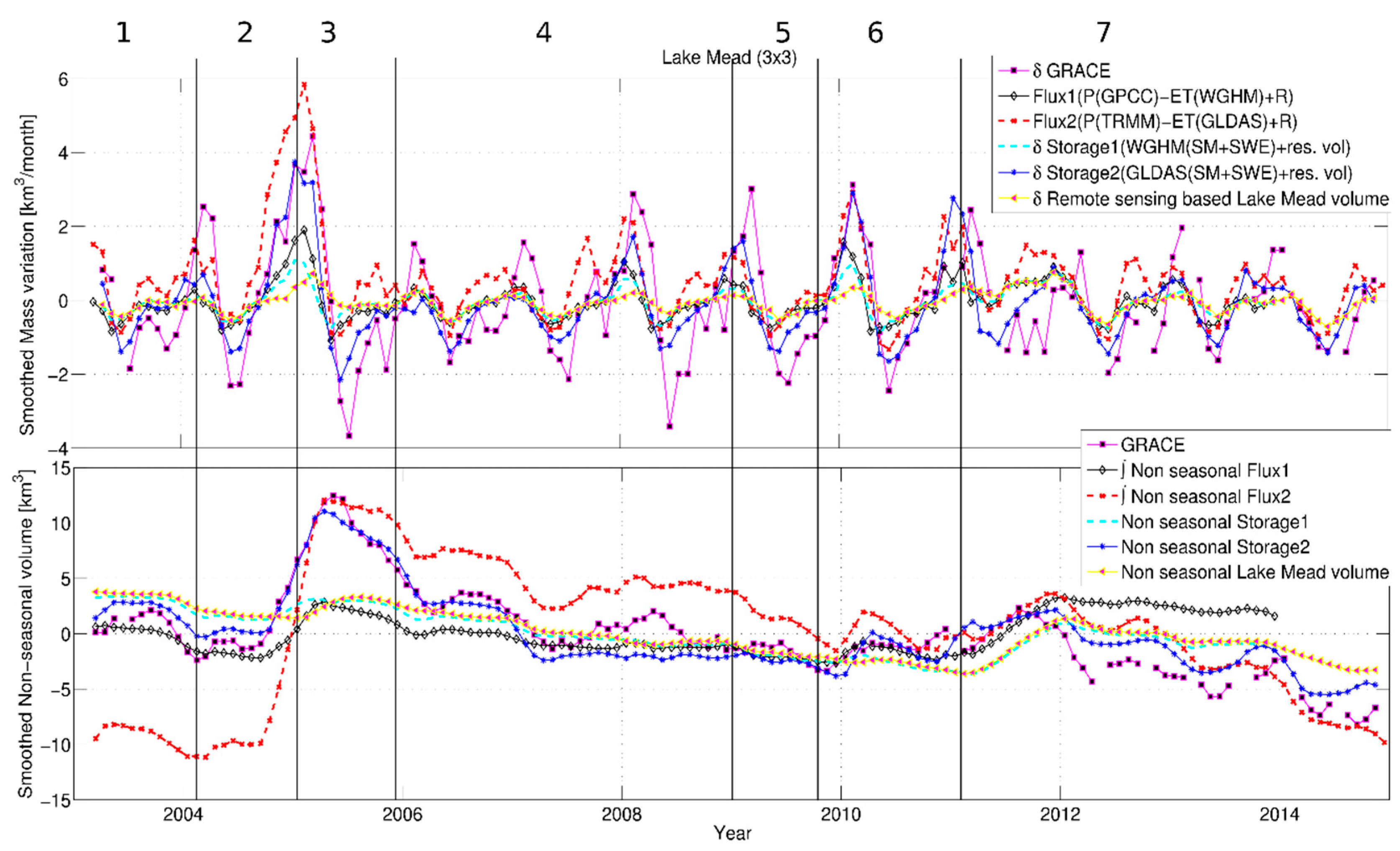
  • This study showed that the inflow-outflow runoff balance predominately drives the volumetric variations in a moderately sized deep reservoir, such as Lake Mead (where open water surface area is in few hundreds of kilometer square and depth is more than 100 m). While the vertical fluxes acting over the reservoir have negligible contributions (blue and green lines in Figure 10 bottom). Therefore, an accurate estimate of reservoir water volume variability may also help to approximate the runoff estimates at a basin level, especially in rivers connected by reservoirs, such as the Colorado River.
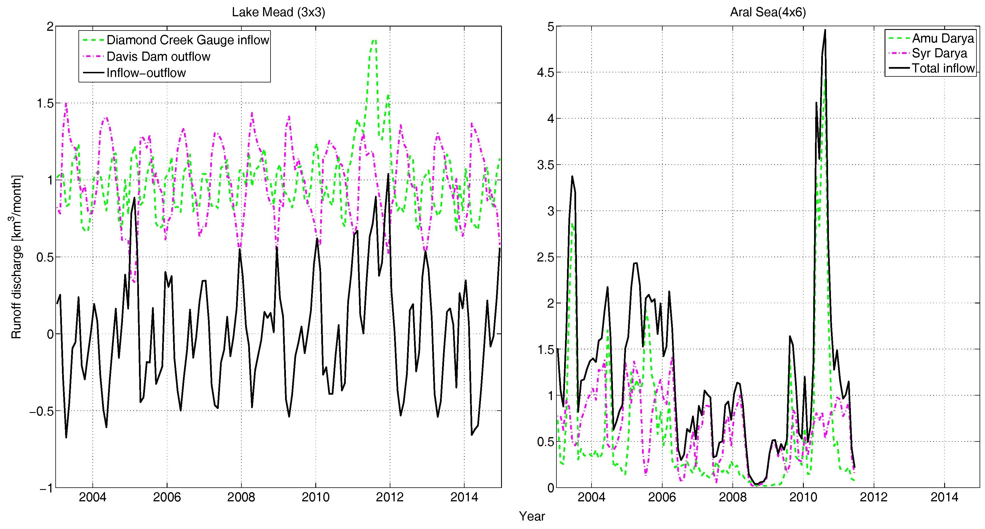
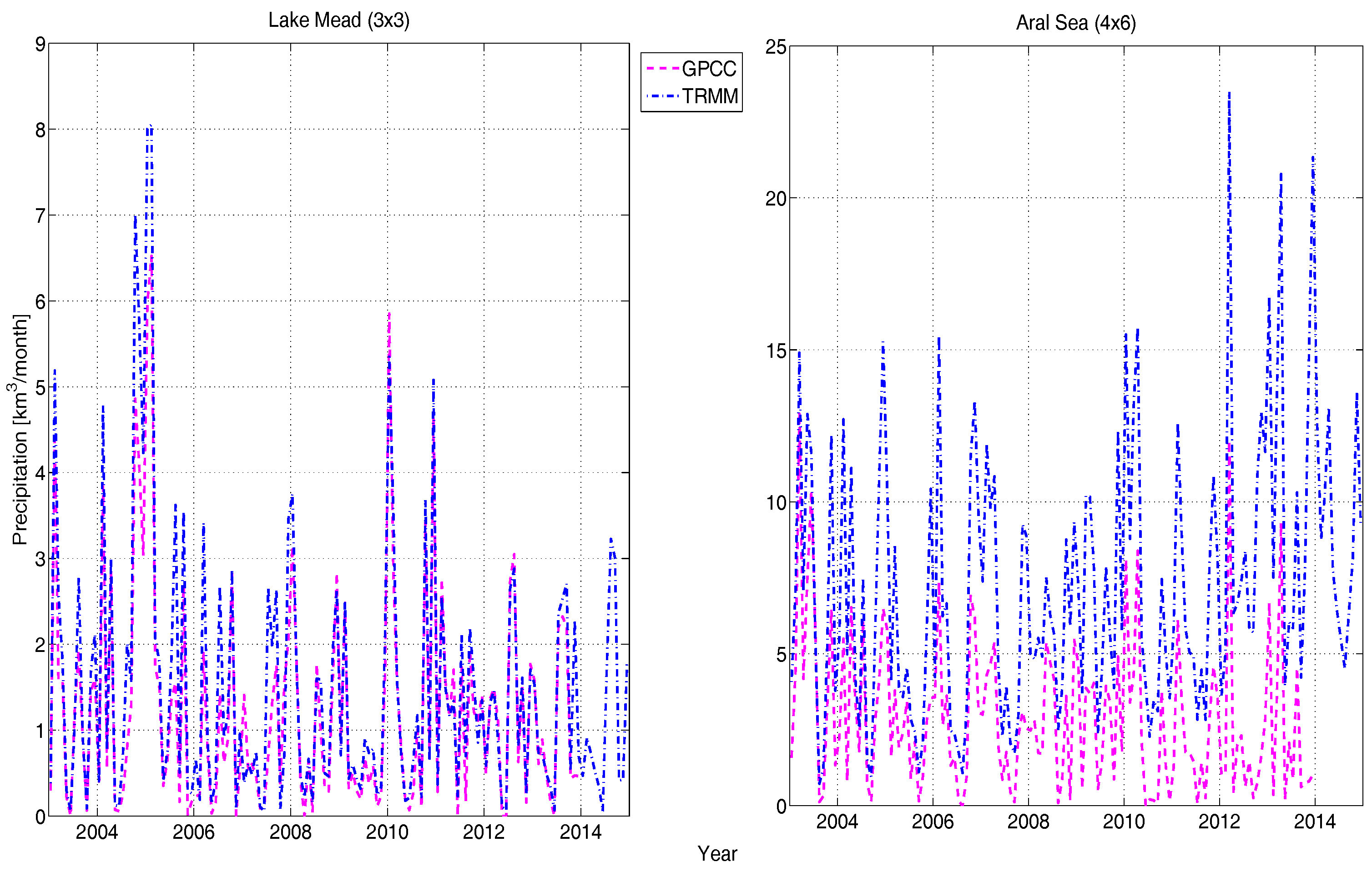
  • The regional variability in the hydrological state of Lake Mead is driven by the combination of runoff (Figure 2 left) and precipitation (Figure 3 left). During the study period, the region experienced mass gains twice: the first time occurred during Period-2 (2004–2005) by additional local rainfall, and the second time by the additional inflow from upstream in Period-6 (2011). This lets us conclude that GRACE is sufficiently sensitive to observe mass changes of Lake Mead if the magnitude of change is large.
  • In the study, ΔTWS observed by GRACE is compared to the estimated hydrological variations in fluxes and storages within the study area. The study showed that the long-term net flux estimation has a larger uncertainty than the total storage, due to the existing larger uncertainties in the vertical fluxes and error propagation through integration. The hybrid approach combining remote sensing-based reservoir volume estimates with hydrological model outputs provides a better possibility for the estimation of total mass change than hydrological models alone.
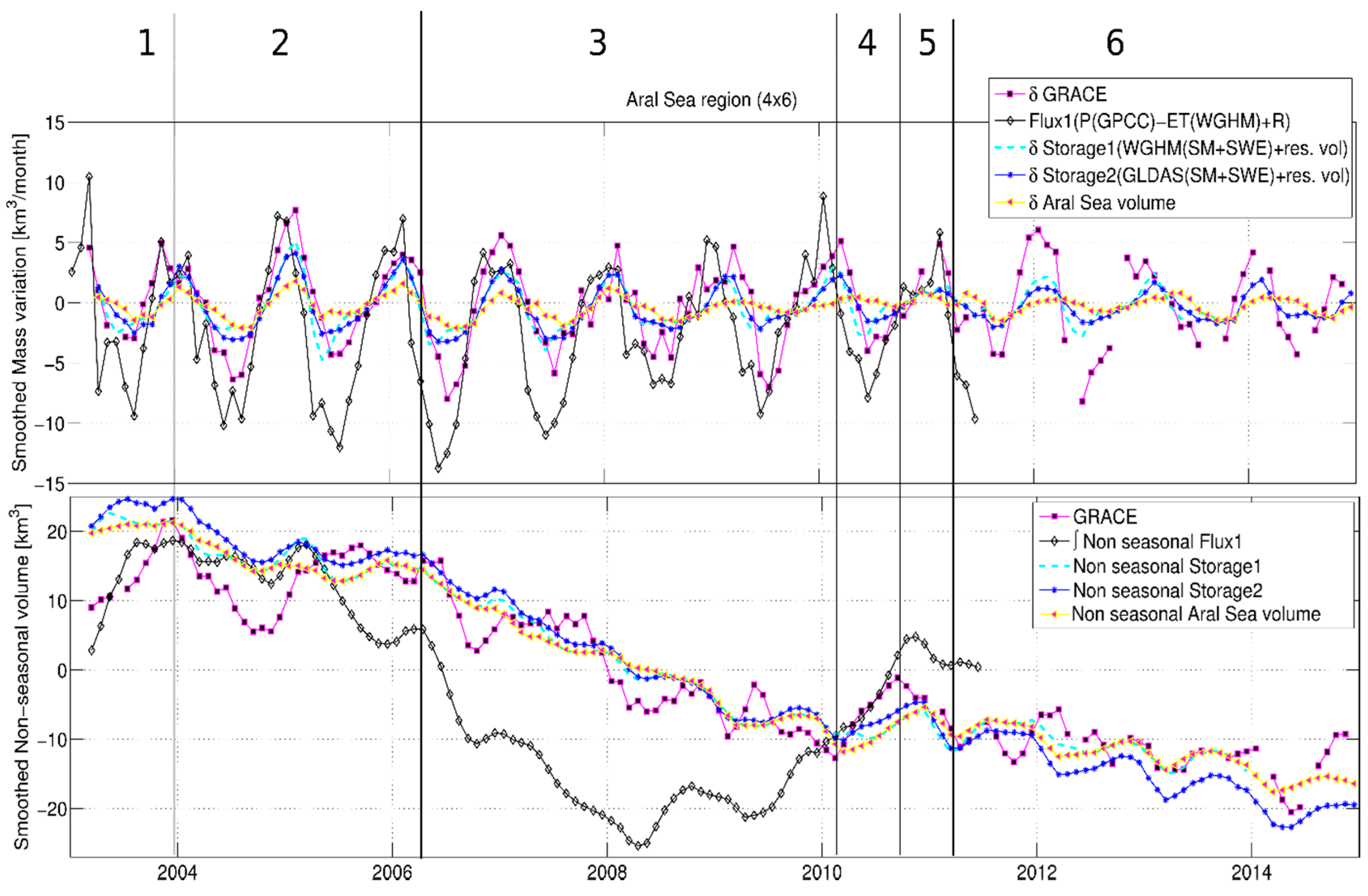
  • The non-seasonal mass depletion in the Aral Sea region observed by GRACE is mainly driven by the reservoir mass loss because SWE is almost stationary (Figure 6 right) and SM has a limited non-seasonal trend (Figure 7 right). This lets us conclude that the causes of mass variations in the region are not local and are driven by upstream water abstraction. On the other hand, the Lake Mead region features almost similar inter-annual variations in SM, SWE, and the reservoir, allowing us to conclude that most of the mass variations are local (except the 2012 inflow anomaly) and climatically driven.
  • Since the Aral Sea has changed dramatically in shape and size, the entire hydrological characteristics of the region have been affected. Therefore, for this region, both models inaccurately determine most of the parameters and no reliable in-situ data are available. Hence, for poorly monitored regions such as the Aral Sea, where reliable data is limited, accurate reservoir storage estimates and GRACE-based mass change analysis can greatly improve the understanding of the hydrological state of the region.

Acknowledgments

This study has been supported by the German Research Foundation (DFG) through the project Clivar-Hydro of TUM’s International Graduate School of Science and Engineering (IGSSE). The authors wish to express appreciation to the United States Bureau of Reclamation (USBR) and Boulder Canyon Operations Office for providing in-situ data for Lake Mead and GLDAS data providers for promptly replying to all queries. The GRACE data are available at http://grace.jpl.nasa.gov, supported by the NASA MEaSUREs Program. The Noah GLDAS data used in this study were acquired as part of the mission of NASA’s Earth Science Division and archived and distributed by the Goddard Earth Sciences (GES) Data and Information Services Center (DISC). The authors are thankful to J.F. Cretaux and four anonymous reviewers for their constructive comments to improve the quality of the manuscript.

Author Contributions

A.S. conceptualized the idea of the computation of an overall water budget of the lake dominated regions through different approaches. A.E. provided the EWH from mascon GRACE solution matrices and wrote a paragraph on mascon theory. A.G. provided the WGHM output matrices and discussed the results. F.S. being the principal investigator of the project provided the necessary guidelines. The creation of figures and the writing of the first manuscript has been done by A.S. All the co-authors helped in the improvement of the manuscript through constructive comments.

Conflicts of Interest

The authors declare no conflict of interest. The funding sponsors had no role in the design of the study; in the collection, analyses, or interpretation of data; in the writing of the manuscript, and in the decision to publish the results.

References

  1. Gleick, P.H. Water in Crisis: A Guide to the World’s Fresh Water Resources; Oxford University Press: New York, NY, USA, 1993. [Google Scholar]
  2. Hall, A.C.; Schumann, G.J.P.; Bamber, J.L.; Bates, P.D. Tracking water level changes of the Amazon Basin with space-borne remote sensing and integration with large scale hydrodynamic modelling: A review. Phys. Chem. Earth Parts ABC 2011, 36, 223–231. [Google Scholar] [CrossRef]
  3. Duan, Z.; Bastiaanssen, W.G.M. Estimating water volume variations in lakes and reservoirs from four operational satellite altimetry databases and satellite imagery data. Remote Sens. Environ. 2013, 134, 403–416. [Google Scholar] [CrossRef]
  4. Zhang, J.; Xu, K.; Yang, Y.; Qi, L.; Hayashi, S.; Watanabe, M. Measuring water storage fluctuations in Lake Dongting, China, by Topex/Poseidon satellite altimetry. Environ. Monit. Assess. 2006, 115, 23–37. [Google Scholar] [CrossRef] [PubMed]
  5. Shiklomanov, A.I.; Lammers, R.B.; Vörösmarty, C.J. Widespread decline in hydrological monitoring threatens Pan-Arctic Research. Eos Trans. Am. Geophys. Union 2002, 83. [Google Scholar] [CrossRef]
  6. Rodell, M.; Chen, J.; Kato, H.; Famiglietti, J.S.; Nigro, J.; Wilson, C.R. Estimating groundwater storage changes in the Mississippi River basin (USA) using GRACE. Hydrogeol. J. 2006, 15, 159–166. [Google Scholar] [CrossRef]
  7. Famiglietti, J.S.; Lo, M.; Ho, S.L.; Bethune, J.; Anderson, K.J.; Syed, T.H.; Swenson, S.C.; de Linage, C.R.; Rodell, M. Satellites measure recent rates of groundwater depletion in California’s Central Valley. Geophys. Res. Lett. 2011, 38. [Google Scholar] [CrossRef]
  8. De Paiva, R.C.D.; Buarque, D.C.; Collischonn, W.; Bonnet, M.P.; Frappart, F.; Calmant, S.; Bulhões Mendes, C.A. Large-scale hydrologic and hydrodynamic modeling of the Amazon River basin. Water Resour. Res. 2013, 49, 1226–1243. [Google Scholar] [CrossRef] [Green Version]
  9. Frappart, F.; Papa, F.; Güntner, A.; Werth, S.; da Silva, J.S.; Tomasella, J.; Seyler, F.; Prigent, C.; Rossow, W.B.; Calmant, S.; et al. Satellite-based estimates of groundwater storage variations in large drainage basins with extensive floodplains. Remote Sens. Environ. 2011, 115, 1588–1594. [Google Scholar] [CrossRef] [Green Version]
  10. Papa, F.; Frappart, F.; Malbeteau, Y.; Shamsudduha, M.; Vuruputur, V.; Sekhar, M.; Ramillien, G.; Prigent, C.; Aires, F.; Pandey, R.K.; et al. Satellite-derived surface and sub-surface water storage in the Ganges–Brahmaputra River Basin. J. Hydrol. Reg. Stud. 2015, 4, 15–35. [Google Scholar] [CrossRef]
  11. Singh, A.; Kumar, U.; Seitz, F. Remote sensing of storage fluctuations of poorly gauged reservoirs and state space model (ssm)-based estimation. Remote Sens. 2015, 7, 17113–17134. [Google Scholar] [CrossRef]
  12. Rosenberg, E.A.; Clark, E.A.; Steinemann, A.C.; Lettenmaier, D.P. On the contribution of groundwater storage to interannual streamflow anomalies in the Colorado River basin. Hydrol. Earth Syst. Sci. 2013, 17, 1475–1491. [Google Scholar] [CrossRef]
  13. Barsugli, J.J.; Nowak, K.; Rajagopalan, B.; Prairie, J.R.; Harding, B. Comment on “When will Lake Mead go dry?” by T.P. Barnett and D.W. Pierce. Water Resour. Res. 2009, 45. [Google Scholar] [CrossRef]
  14. European Space Agency (ESA) Data User Element. Available online: http://due.esrin.esa.int/page_globcover.php (accessed on 10 May 2016).
  15. Central Asia (CA) Water Info. Available online: http://www.cawater-info.net/ (accessed on 12 November 2011).
  16. Rodell, M.; Houser, P.R.; Jambor, U.E.A.; Gottschalck, J. The global land data assimilation system. Bull. Am. Meteorol. Soc. 2004, 85, 381–394. [Google Scholar] [CrossRef]
  17. Simple Subset Wizard (SSW): Search for Data Sets. Available online: http://disc.sci.gsfc.nasa.gov/SSW/#keywords= (accessed on 10 November 2016).
  18. Huffman, G.J.; Bolvin, D.T.; Nelkin, E.J.; Wolff, D.B.; Adler, R.F.; Gu, G.; Hong, Y.; Bowman, K.P.; Stocker, E.F. The TRMM multisatellite precipitation analysis (TMPA): Quasi-global, multiyear, combined-sensor precipitation estimates at fine scales. J. Hydrometeorol. 2007, 8, 38–55. [Google Scholar] [CrossRef]
  19. Döll, P.; Kaspar, F.; Lehner, B. A global hydrological model for deriving water availability indicators: Model tuning and validation. J. Hydrol. 2003, 270, 105–134. [Google Scholar] [CrossRef]
  20. Müller Schmied, H.; Eisner, S.; Franz, D.; Wattenbach, M.; Portmann, F.T.; Flörke, M.; Döll, P. Sensitivity of simulated global-scale freshwater fluxes and storages to input data, hydrological model structure, human water use and calibration. Hydrol. Earth Syst. Sci. 2014, 18, 3511–3538. [Google Scholar] [CrossRef]
  21. Small, E.E.; Sloan, L.C.; Hostetler, S.; Giorgi, F. Simulating the water balance of the Aral Sea with a coupled regional climate-lake model. J. Geophys. Res. Atmos. 1999, 104, 6583–6602. [Google Scholar] [CrossRef]
  22. Small, E.E.; Giorgi, F.; Sloan, L.C.; Hostetler, S. The effects of desiccation and climatic change on the hydrology of the Aral Sea. J. Clim. 2001, 14, 300–322. [Google Scholar] [CrossRef]
  23. Cretaux, J.F.; Letolle, R.; Bergé-Nguyen, M. History of Aral Sea level variability and current scientific debates. Glob. Planet. Chang. 2013, 110, 99–113. [Google Scholar] [CrossRef]
  24. Papa, F.; Prigent, C.; Rossow, W.B.; Legresy, B.; Remy, F. Inundated wetland dynamics over boreal regions from remote sensing: The use of Topex-Poseidon Dual-frequency radar altimeter observations. Int. J. Remote Sens. 2006, 27, 4847–4866. [Google Scholar] [CrossRef]
  25. Seitz, F.; Schmidt, M.; Shum, C.K. Signals of extreme weather conditions in Central Europe in GRACE 4-D hydrological mass variations. Earth Planet. Sci. Lett. 2008, 268, 165–170. [Google Scholar] [CrossRef]
  26. Forootan, E.; Didova, O.; Kusche, J.; Löcher, A. Comparisons of atmospheric data and reduction methods for the analysis of satellite gravimetry observations. J. Geophys. Res. Solid Earth 2013, 118, 2382–2396. [Google Scholar] [CrossRef]
  27. Jiang, H.; Feng, M.; Zhu, Y.; Lu, N.; Huang, J.; Xiao, T. An automated method for extracting rivers and lakes from Landsat imagery. Remote Sens. 2014, 6, 5067–5089. [Google Scholar] [CrossRef]
  28. Eicker, A.; Schumacher, M.; Kusche, J.; Döll, P.; Schmied, H.M. Calibration/data assimilation approach for integrating GRACE data into the WaterGAP Global Hydrology Model (WGHM) using an ensemble Kalman filter: First results. Surv. Geophys. 2014, 35, 1285–1309. [Google Scholar] [CrossRef]
  29. Schumacher, M.; Eicker, A.; Kusche, J.; Schmied, H.M.; Döll, P. Covariance analysis and sensitivity studies for GRACE assimilation into WGHM. In International Association of Geodesy Symposia; Rizos, C., Ed.; Springer: Berlin/Heidelberg, Germany, 2015; pp. 1–7. [Google Scholar]
  30. Tangdamrongsub, N.; Steele-Dunne, S.C.; Gunter, B.C.; Ditmar, P.G.; Weerts, A.H. Data assimilation of GRACE terrestrial water storage estimates into a regional hydrological model of the Rhine River basin. Hydrol. Earth Syst. Sci. 2015, 19, 2079–2100. [Google Scholar] [CrossRef]
  31. Swenson, S.; Yeh, P.J.F.; Wahr, J.; Famiglietti, J. A comparison of terrestrial water storage variations from GRACE with in situ measurements from Illinois. Geophys. Res. Lett. 2006, 33. [Google Scholar] [CrossRef]
  32. Swenson, S.; Wahr, J. Monitoring the water balance of Lake Victoria, East Africa, from space. J. Hydrol. 2009, 370, 163–176. [Google Scholar] [CrossRef]
  33. Strassberg, G.; Scanlon, B.R.; Rodell, M. Comparison of seasonal terrestrial water storage variations from GRACE with groundwater-level measurements from the High Plains Aquifer (USA). Geophys. Res. Lett. 2007, 34. [Google Scholar] [CrossRef]
  34. Becker, M.; LLovel, W.; Cazenave, A.; Güntner, A.; Crétaux, J.F. Recent hydrological behavior of the East African great lakes region inferred from GRACE, satellite altimetry and rainfall observations. C. R. Geosci. 2010, 342, 223–233. [Google Scholar] [CrossRef]
  35. Singh, A.; Seitz, F.; Schwatke, C. Application of Multi-Sensor satellite data to observe water storage variations. IEEE J. Sel. Top. Appl. Earth Obs. Remote Sens. 2013, 6, 1502–1508. [Google Scholar] [CrossRef]
  36. Forootan, E.; Rietbroek, R.; Kusche, J.; Sharifi, M.A.; Awange, J.L.; Schmidt, M.; Omondi, P.; Famiglietti, J. Separation of large scale water storage patterns over Iran using GRACE, altimetry and hydrological data. Remote Sens. Environ. 2014, 140, 580–595. [Google Scholar] [CrossRef]
  37. Aus der Beek, T.; Voß, F.; Flörke, M. Modelling the impact of Global Change on the hydrological system of the Aral Sea basin. Phys. Chem. Earth Parts ABC 2011, 36, 684–695. [Google Scholar] [CrossRef]
  38. Long, D.; Longuevergne, L.; Scanlon, B.R. Global analysis of approaches for deriving total water storage changes from GRACE satellites. Water Resour. Res. 2015, 51, 2574–2594. [Google Scholar] [CrossRef] [Green Version]
  39. Watkins, M.M.; Wiese, D.N.; Yuan, D.N.; Boening, C.; Landerer, F.W. Improved methods for observing Earth’s time variable mass distribution with GRACE using spherical cap mascons. J. Geophys. Res. Solid Earth 2015, 120, 2648–2671. [Google Scholar] [CrossRef]
  40. Wiese, D.N. GRACE Monthly Land Water Mass Grids Netcdf Release 5.0|PO.DAAC. Available online: https://podaac.jpl.nasa.gov/dataset/TELLUS_LAND_NC_RL05 (accessed on 31 March 2016).
  41. Studying Earth’s Gravity. Available online: http://grace.jpl.nasa.gov/ (accessed on 10 November 2016).
  42. Swenson, S.; Chambers, D.; Wahr, J. Estimating geocenter variations from a combination of GRACE and ocean model output. J. Geophys. Res. Solid Earth 2008, 113. [Google Scholar] [CrossRef]
  43. Cheng, M.; Tapley, B.D.; Ries, J.C. Deceleration in the Earth’s oblateness. J. Geophys. Res. Solid Earth 2013, 118, 740–747. [Google Scholar] [CrossRef]
  44. Geruo, A.; Wahr, J.; Zhong, S. Computations of the viscoelastic response of a 3-D compressible Earth to surface loading: An application to Glacial Isostatic Adjustment in Antarctica and Canada. Geophys. J. Int. 2013, 192, 557–572. [Google Scholar]
  45. Longuevergne, L.; Wilson, C.; Scanlon, B.R.; Crétaux, J.F. GRACE water storage estimates for the Middle East and other regions with significant reservoir and lake storage. Hydrol. Earth Syst. Sci. 2013, 17, 4817–4830. [Google Scholar] [CrossRef] [Green Version]
  46. Overview—Monthly Mass Grids. Available online: http://grace.jpl.nasa.gov/data/monthly-mass-grids (accessed on 10 October 2016).
  47. Boulder Canyon Operations Office|Lower Colorado Region|Bureau of Reclamation. Available online: http://www.usbr.gov/lc/region/g4000/wtracct.html (accessed on 10 November 2016).
  48. United States Geological Survey (USGS) Water Data for the Nation. Available online: http://waterdata.usgs.gov/nwis (accessed on 10 November 2016).
  49. Rechard, P.A. Determining bank storage of Lake Mead. J. Irrig. Drain. Div. 1965, 91, 141–158. [Google Scholar]
  50. Lindsey, R. World of Change: Water Level in Lake Powell —Feature Articles. Available online: http://earthobservatory.nasa.gov/Features/WorldOfChange/lake_powell.php (accessed on 19 July 2016).
  51. Lindsey, R. World of Change: Shrinking Aral Sea —Feature Articles. Available online: http://earthobservatory.nasa.gov/Features/WorldOfChange/aral_sea.php (accessed on 19 July 2016).
  52. Aladin, N.V.; Plotnikov, I.S.; Micklin, P.; Ballatore, T. The Aral Sea: Water level, salinity and long-term changes in biological communities of an endangered ecosystem-past, present and future. Nat. Resour. Environ. Issues 2009, 15, 177–183. [Google Scholar]
  53. Abelen, S.; Seitz, F. Relating satellite gravimetry data to global soil moisture products via data harmonization and correlation analysis. Remote Sens. Environ. 2013, 136, 89–98. [Google Scholar] [CrossRef]
  54. Yin, X.; Gruber, A.; Arkin, P. Comparison of the GPCP and CMAP merged gauge—Satellite monthly precipitation products for the period 1979–2001. J. Hydrometeorol. 2004, 5, 1207–1222. [Google Scholar] [CrossRef]
  55. Negrón Juárez, R.I.; Li, W.; Fu, R.; Fernandes, K.; de Oliveira Cardoso, A. Comparison of precipitation datasets over the Tropical South American and African continents. J. Hydrometeorol. 2009, 10, 289–299. [Google Scholar] [CrossRef]
  56. Shin, D.B.; Kim, J.H.; Park, H.J. Agreement between monthly precipitation estimates from TRMM satellite, NCEP reanalysis, and merged gauge-satellite analysis. J. Geophys. Res. Atmospheres 2011, 116. [Google Scholar] [CrossRef]
  57. Chen, J.; Li, J.; Zhang, Z.; Ni, S. Long-term groundwater variations in Northwest India from satellite gravity measurements. Glob. Planet. Chang. 2014, 116, 130–138. [Google Scholar] [CrossRef]
  58. Richey, A.S.; Thomas, B.F.; Lo, M.H.; Reager, J.T.; Famiglietti, J.S.; Voss, K.; Swenson, S.; Rodell, M. Quantifying renewable groundwater stress with GRACE. Water Resour. Res. 2015, 51, 5217–5238. [Google Scholar] [CrossRef] [PubMed]
  59. Chen, J.; Famigliett, J.S.; Scanlon, B.R.; Rodell, M. Groundwater storage changes: Present status from GRACE observations. Surv. Geophys. 2015, 37, 397–417. [Google Scholar] [CrossRef]
  60. Castle, S.L.; Thomas, B.F.; Reager, J.T.; Rodell, M.; Swenson, S.C.; Famiglietti, J.S. Groundwater depletion during drought threatens future water security of the Colorado River Basin. Geophys. Res. Lett. 2014, 41, 5904–5911. [Google Scholar] [CrossRef] [PubMed]
Figure 1. Study box for the Lake Mead region and the Aral Sea region. River discharge: 1 = Colorado River inflow, 2 = Virgin River, 3 = Muddy River, 4 = Colorado River outflow, 5 = Syr Darya and 6 = Amu Darya.
Remotesensing 08 00953 g001
Figure 2. Runoff: (left) Lake Mead and (right) The Aral Sea.
Remotesensing 08 00953 g002
Figure 3. Precipitation: (left) The Lake Mead region and (right) The Aral Sea region.
Remotesensing 08 00953 g003
Figure 4. ET: (left) The Lake Mead region and (right) The Aral Sea region.
Remotesensing 08 00953 g004
Figure 5. Mean reduced reservoir volume: (left) Lake Mead and (right) The Aral Sea.
Remotesensing 08 00953 g005
Figure 6. Mean reduced Snow Water Equivalent: (left) The Lake Mead region and (right) The Aral Sea region.
Remotesensing 08 00953 g006
Figure 7. Mean reduced Soil Moisture: (left) The Lake Mead region and (right) The Aral Sea region.
Remotesensing 08 00953 g007
Figure 8. Gravity Recovery and Climate Experiment (GRACE)-derived trend of the equivalent water height (meter/year) between 2003 and 2014. The size of the study area was chosen according to the mascon grid. (left) The Lake Mead region is 3° × 3° where Lake Mead is located at the center. (right) The Aral Sea region is 4° × 6°covering the entire lake and two mascon grid cells.
Remotesensing 08 00953 g008
Figure 9. GRACE-derived mass variations with the uncertainty range of the measurements as provided by GRACE Tellus: (left) The Lake Mead region, (right) The Aral Sea region
Remotesensing 08 00953 g009
Figure 10. Lake Mead: (top) Net surface runoff of the lake: inflow–outflow and (bottom) Reservoir volume variation compared with the hydrological fluxes.
Remotesensing 08 00953 g010
Figure 11. Lake Mead region (3° × 3°) mass variations observed by net fluxes, net storages, and GRACE: (top) Monthly mass variations and (bottom) Non-seasonal water storage variability. All time series in the lower panel have been reduced for their mean (i.e., mean value over the study period). The large numbers at the top of the figure are the periods of different mass evolution, discussed in Section 4.2. Here symbol δ indicates derivative and indicates integral of the signal.
Remotesensing 08 00953 g011
Figure 12. Aral Sea region (4° × 6°) mass variations observed by net flux, net storages, and GRACE: (top) Monthly mass variations and (bottom) Non-seasonal water storage variability. All time series in the lower panel have been reduced for their mean (i.e., mean value over the study period). The large numbers at the top of the figure are the periods of different mass evolution, discussed in Section 4.3. Here symbol δ indicates derivative and indicates integral of the signal.
Remotesensing 08 00953 g012
Figure 13. Total water storage (TWS) observed by GRACE compared with the best estimates and the reservoir volume: (left) The Lake Mead region and (right) The Aral Sea region.
Remotesensing 08 00953 g013
Table 1. Correlation of the GRACE signal with the net fluxes (combining in-situ runoff with different vertical fluxes, i.e., Flux-1 (precipitation (P) from Global Precipitation Climatology Centre (GPCC) and evapotranspiration (ET) from Global Land Data Assimilation System (GLDAS)) and Flux-2 (P from Tropical Rainfall Measuring Mission (TRMM) and ET from WaterGAP Global Hydrological Model (WGHM)), and hybrid storages (combining remote sensing based reservoir volume estimate with the SM and SWE from global hydrological models, i.e., Storage-1 (WGHM) and Storage-2 (GLDAS)). Lag 0 means instantaneous correlation between the derivative of GRACE and the flux. Lag 1 means a lag of 1 month with respect to the flux.
Signals (Including Seasonal Component)The Lake Mead Region (3 × 3)The Aral Sea Region (4 × 6)
CorrelationRMSE (km3)CorrelationRMSE (km3)
Lag 0Lag 1Lag 0Lag 1
δ GRACE-Flux-10.580.801.30.760.84.2
δ GRACE-Flux-20.630.761.3---
GRACE-Storage-10.58-3.70.87-6.5
GRACE-Storage-20.87-2.30.88-7
GRACE-Reservoir0.60 40.82-7.8

