Using Landsat, MODIS, and a Biophysical Model to Evaluate LST in Urban Centers

Abstract

In this paper, we assessed and compared land surface temperature (LST) in urban centers using data from Landsat, MODIS, and the Simple Biosphere model (SiB2). We also evaluated the sensitivity of the model’s LST to different land cover types, fractions (percentages), and emissivities compared to reference points derived from Landsat thermal data. This was demonstrated in three climatologically- and morphologically-different cities of Atlanta, GA, New York, NY, and Washington, DC. Our results showed that in these cities SiB2 was sensitive to both the emissivity and the land cover type and fraction, but much more sensitive to the latter. The practical implications of these results are rather significant since they imply that the SiB2 model can be used to run different scenarios for evaluating urban heat island (UHI) mitigation strategies. This study also showed that using detailed emissivities per land cover type and fractions from Landsat-derived data caused a convergence of the model results towards the Landsat-derived LST for most of the studied cases. This study also showed that SiB2 LSTs are closer in magnitude to Landsat-derived LSTs than MODIS-derived LSTs. It is important, however, to emphasize that both Landsat and MODIS LSTs are not direct observations and, as such, do not represent a ground truth. More studies will be needed to compare these results to in situ LST data and provide further validation.

1. Introduction

Land surface temperature (LST) is of fundamental importance in many land surface physical processes. It is a key indicator of climate change, vegetation monitoring, and urban climate [1,2,3]. Currently, satellite thermal infrared sensors provide global coverage of different spatial resolution data that can be used to estimate land surface temperatures. However these are inadequate to characterize LST temporal evolution at daily or hourly time scales. Additionally, the use of satellite-derived LST can be limited because of cloud masking and calibration issues. On the other hand, model-simulated land surface temperatures can offer homogeneous spatial coverage and desired temporal resolution of the diurnal cycle. The main aim of this study is to evaluate the LST in urban centers, and for that we used two different approaches: one, by using purely remote sensing, and the other by using physical modeling assimilated with remotely-sensed data.

In this paper, we compare and assess LST in urban centers using datasets from Landsat, MODIS, and the Simple Biosphere model (SiB2) of Sellers et al. [4] as modified by Bounoua et al. [5]. We also evaluate the sensitivity of SiB2 LST to different land cover (LC) types, fractions (percentages), and emissivities compared to same baseline/reference points derived from Landsat thermal data. This was demonstrated in three climatologically- and morphologically-different cities of Atlanta, GA, New York, NY, and Washington, DC.

Large errors in net longwave radiation due to inaccurate emissivity may occur where there are large differences between upward and downward longwave radiation, and where the surface emissivity greatly departs from unity [6]. For example, sensitivity studies conducted by Jin and Liang [6] on the National Center for Atmospheric Research (NCAR) Community Land Model version 2 (CLM2) and coupled NCAR community atmosphere models showed that large impacts of surface emissivity occur over deserts, with changes up to 1–2 °C in ground temperature, surface skin temperature, and 2-m surface air temperature, as well as evident changes in sensible and latent heat fluxes. In this study, we evaluate the SiB2 model’s sensitivity to different LC types, fractions, and emissivity in three climatologically- and morphologically-different cities.

2. Description of MODIS LST and Landsat Thermal Data

The MODIS data collections are derived from both the NASA Terra and Aqua MODIS instruments, temporally spanning from 2000 until the present. The calibration for the 16 thermal emissive bands is conducted on-orbit using observations of a temperature-controlled blackbody and deep space [7]. Terra descends (ascends) the equator around 10:30 am (10:30 pm) local time, while Aqua descends (ascends) the equator at 1:30 pm (1:30 am) local time. MODIS instruments provide a number of environmental products, including land cover/land use change, net primary productivity, leaf area index, emissivity values, and surface temperature. The Terra MOD11A1 product used in this study for downscaling is the daily daytime LST product collected by the Terra instrument at spatial resolutions of 1 km over global land surfaces under clear-sky conditions (Level 3, Collection 5). This product is tile-based and gridded in the sinusoidal projection and is generated using the split-window algorithm [8,9], which uses bands 31 and 32 of MODIS’s 36 spectral bands.

The Landsat satellite series has been providing continuous high-resolution imagery since the launch of Landsat 1 in 1972. Landsat platforms 4–7, compared to earlier satellites, had lower orbits, higher spatial resolution, faster repeat cycle, and the addition of the thematic mapper (TM) for Landsat 4 and 5 [10]. TM data collected from Landsat 5 is one of the most actively used datasets for environmental studies [11]. The spectral range of Landsat 5 TM is from 0.45 μm to 12.50 μm for bands 1–6 [11]. For this study, thermal band 6 was used for LST retrievals. Due to the limitation of processing only one thermal band, temperature/emissivity separation requires the development of other methods to derive emissivity estimates for various surface types [11]. We used the Landsat-derived National Land Cover Dataset (NLCD) as the basis for estimating emissivity for each of several land surface types [12].

Landsat 7 dropped the multispectral scanner system (MSS) sensor and only included the enhanced thematic mapper plus (ETM⁺) sensor. This sensor’s spectral range is similar to the Landsat 5 TM ranging from 0.45 μm to 12.50 μm, including a 60 m spatial resolution in the thermal infrared band. The thermal band from Landsat 7 ETM⁺ has been found to provide reliable estimates of LST in urban areas with high differentiation among surface types [12,13,14].

The overpass times of the Landsat images over our study areas range from 10:30 am-noon local time, thus, we used the Terra platform, which has a morning overpass time of ~10:30 am, rather than Aqua MODIS images in this study.

3. Study Areas and Periods

The methods developed in this study have been applied for Atlanta, GA, New York, NY, and Washington, DC, using Landsat, MODIS, and SiB2 model data from 2001. The choice of the cities is dictated by the desire to evaluate the amplitude of the surface urban heat island (SUHI) along the south-north temperature gradient and by the availability of data in these cities.

Table 1. Dates of the cloud-free images that were used in this study.

Study Area	Date
Atlanta, GA	2001: 2 January **, 10 January *, 26 January *, 19 February **, 7 March **, 23 March **, 16April *, 2 May *, 18 May *, 26 May **, 22 August *, 15 September **, 23 September *, 1 October **, 17 October **, 25 October *, 10 November *, 4 December **, 20 December **.
New York, NY	2001: 12 March *, 28 March *, 14 April **, 29 April *, 30 April **, 7 May **, 15 May *, 31 May *, 12 September **, 13 September *, 7 October **, 22 October *, 8 November **, 1 December **, 26 December **.
Washington, DC	2001: 2 February **, 19 March *, 4 April *, 28 April **, 9 July *, 2 August **, 26 August *, 5 October **, 13 October *, 22 October **, 29 October *, 6 November **, 14 November *.

* Landsat 5 TM, ** Landsat 7 ETM⁺.

shows the dates of the cloud-free images used for method development or validation. The acquired Landsat scenes are characterized by very clear atmospheric conditions, and the images were acquired through the USGS Earth Resource Observation Systems Data Center, which corrected the radiometric and geometrical distortions of the images to a quality level of 1 G before delivery [12,15]. Since this study used images acquired on clear days and over small areas, we believe that the spatial variations due to the lack of atmospheric correction was minimized as other LST estimation studies have suggested [12,15,16,17]. Additionally, this study focused on a comparison among methods applied to the same Landsat TM scenes, thus, all cases would have similar atmospheric effects, and the effects of not performing atmospheric corrections on the differences of results from these methods would be small. 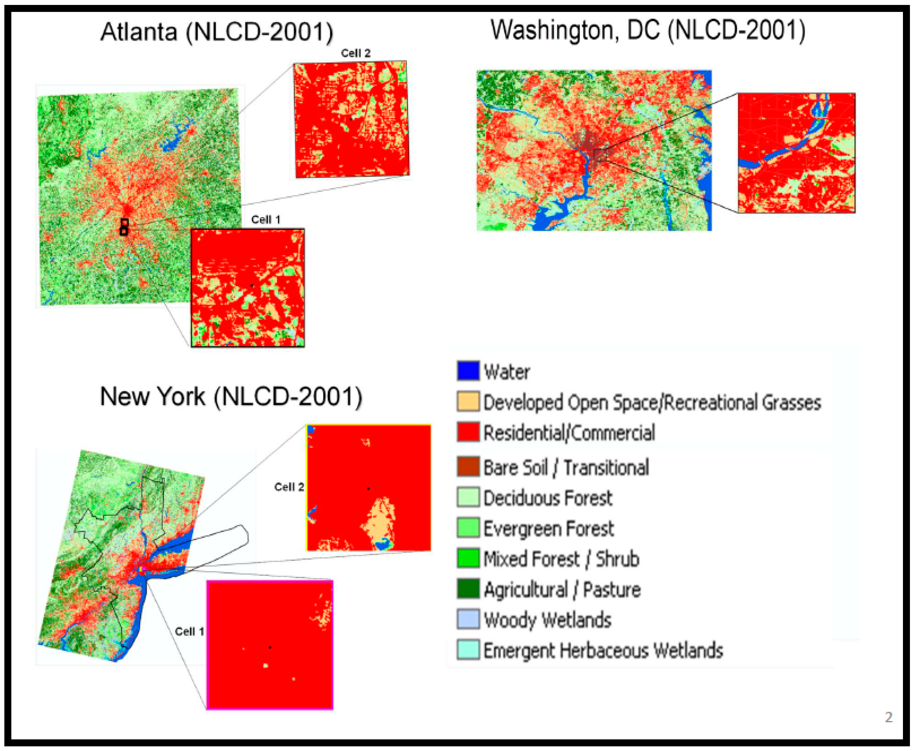Figure 1 shows the spatial domain of our study areas and the LC within those areas.

4. Methods

4.1. SiB2 Model-Derived LST

In this paper, a fusion of Landsat and MODIS data was used in the Simple Biosphere model (SiB2) of Sellers et al. [4] as modified by Bounoua et al. [5,18,19] to assess the impact of different land cover (LC) types/fractions and emissivity on land surface temperature (LST) and the urban heat island (UHI) phenomenon in the studied cities. SiB2 is a biophysically-based soil vegetation atmosphere transfer (SVAT) model that computes the exchanges of carbon, energy, water, and momentum between the land surface and the atmosphere, accounting for 12 vegetation types [4,5]. The model is fed with a land cover map, topography, and soil maps, as well as time-independent parameters characterizing the physiological, optical, and morphological properties of the vegetation and soil [4]. The MODIS-based biophysical products at 500 m × 500 m spatial resolution and eight-day time-interval were used to describe the vegetation phenology within a climate modeling grid (CMG) of 0.05° × 0.05° of latitude and longitude (approximately 5 km × 5 km) [4,5]. In addition to predicting water stores and the canopy stomatal resistance, the model also predicts three temperatures describing the canopy, the ground surface, and the deep soil, using a coupled carbon-energy-water balance [4,5]. The model is driven by a two-stream, short- and long-wave radiation, direct and diffuse, convective and large scale precipitation, specific humidity, surface air temperature, surface pressure, and wind speed at some reference height above the canopy and returns components of the carbon, energy, and water fluxes. The model was run for three scenarios to evaluate its sensitivity of LST estimation to different LC types/fractions and emissivity. These scenarios were:

(1)

The Landsat-based impervious surface area (ISA) from the National Land Cover Dataset (NLCD) [20] was used to characterize the urban areas at 30 m × 30 m spatial resolution. The ISA data was combined with MODIS LC at 500 m spatial resolution and then aggregated into a 5 km × 5 km CMG. Each CMG may have up to 12 LC classes with their fractions within the CMG obtained from higher-resolution Landsat and MODIS data [18]. In this scenario, the emissivity for all land cover types is set to 1.0. This scenario will be labeled hereafter as “SiB_Fr”.

(2)

The Landsat-based impervious surface area (ISA) from the National Land Cover Dataset (NLCD) [20] was used to characterize the urban areas at 30 m × 30 m spatial resolution, and emissivities based on a look-up table for different LC types [21]. This scenario will be labeled hereafter as “SiB_FrEm”.

(3)

The Landsat-derived LC types from the NLCD dataset [20] was used to characterize the urban areas at 30 m × 30 m spatial resolution, and emissivities based on a look-up table for different LC types [21], but all of the residential/commercial developed classes were aggregated into one urban/build-up class, and all the forests were aggregated into one forests class. This scenario will be labeled hereafter as “SiB_MSFC_FrEM”, where MSFC stands for Marshall Space Flight Center, where this scenario was originally introduced.

The locations of the two 5 km × 5 km cells (Cell 1 and Cell 2) in Atlanta, GA, two 5 km × 5 km cells (Cell 1 and Cell 2) in New York, NY, and one 5 km × 5 km cell in Washington, DC, where our analyses were performed are all shown in Figure 1. The LC types and percentages (fractions multiplied by 100) within those areas are specified in

Table 2. LC types and percentages (fractions multiplied by 100).

Scenarios	LC Types	Atlanta Cell 1	Atlanta Cell 2	New York Cell 1	New York Cell 2	Washington DC
SiB_MSFC_FrEM	Water	0	0	0	1.2	4.41
	Barren	0.5	0	0	0	0
	Grassland	17.5	19.2	1	6.8	17.05
	Urban and Buildup	71.4	73.9	98.9	91.3	70.87
	Mixed Forest	10.6	6.9	0.1	0.7	7.67
SiB_Fr and SiB_FrEm	Water	0	0	0	0.52	0
	ISA	42.77	20.73	71.2	82.23	32.98
	Broadleaf deciduous	0	0	0	0	2.03
	Mixed forest	4.58	15.3		3.67	2.03
	Evergreen needleleaf	0	0	0	0.52	0
	Savannah	52.65	52.85	4.8	0	28.43
	Grassland	0	0	0	0.26	0
	Shrubs and Bare Soil	0	0	0	0.78	0
	Barren	0	0	0	12.02	0
	Crop	0	11.13	24.0	0	34.53

for each scenario.

4.2. Landsat-Derived LST

In order to derive land surface temperature (LST) from Landsat thermal data, we followed a procedure that has been demonstrated by studies, such as Weng et al. [15] and Al-Hamdan et al. [12], which involves the following three steps:

(1)

Converting the digital number of Landsat TM or ETM⁺ TIR band into spectral radiance (W/(m²·sr·μm)):

Radiance = 0.0370588 × DN + 3.20 (For Landsat7 ETM⁺)

Radiance = 0.0553760 × DN + 1.18 (For Landsat5 TM)

(2)

Converting the spectral radiance to an at-satellite brightness temperature (i.e., blackbody temperature, T_B):

T_B = K₂/[ln(K₁/Radiance + 1)]

where “ln” is the natural logarithm, and K₂ and K₁ are pre-launch calibration constants:

K₂ = 1282.71 K K₁ = 666.09 W/(m²·sr·μm)  (for Landsat 7 ETM⁺)

K₂ = 1260.56 K K₁ = 607.76 W/(m²·sr·μm)  (for Landsat 5 TM)

(3)

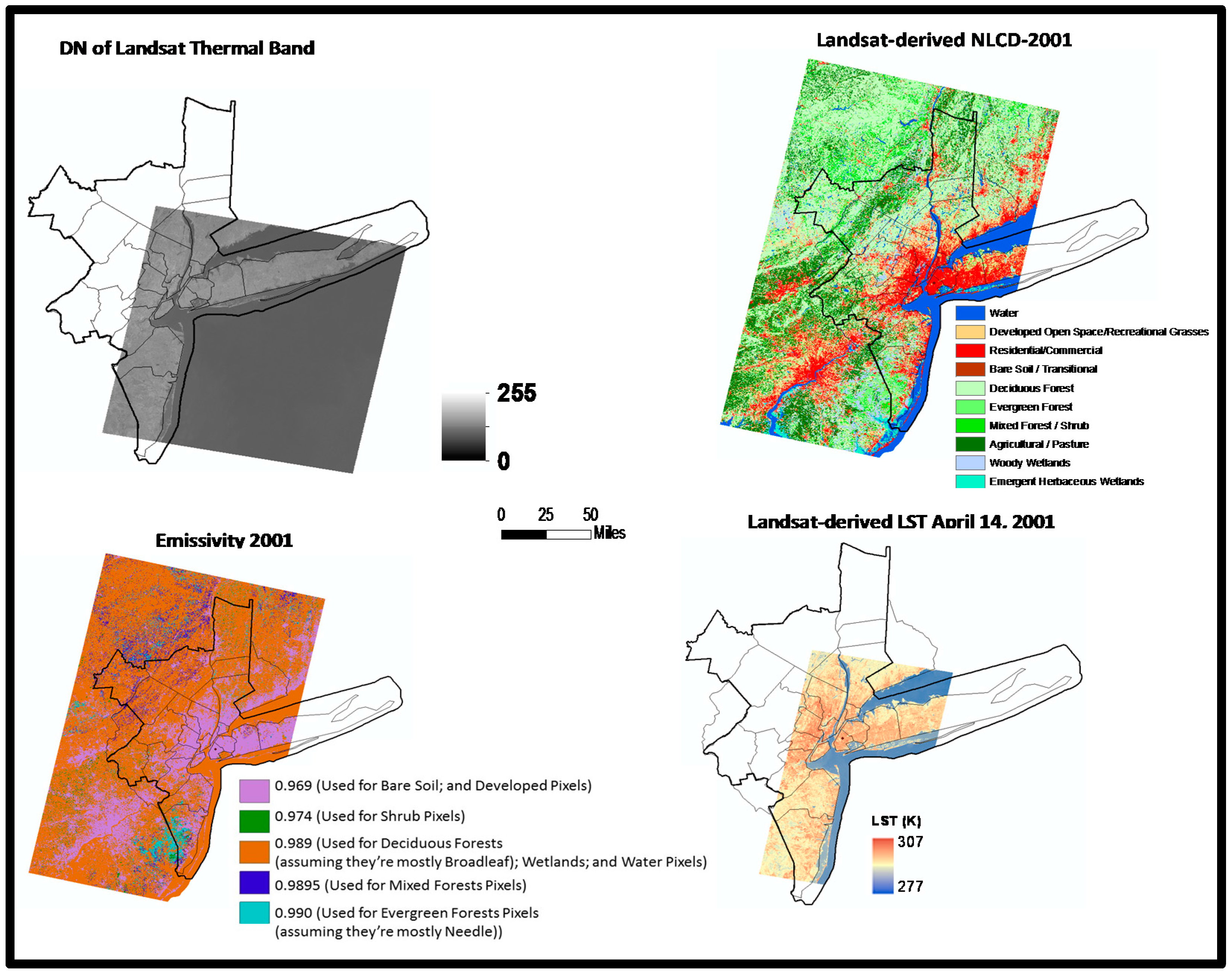
Converting the blackbody temperature to the land surface temperature (LST) which involves correcting for spectral emissivity according to the nature of the land cover. We identified the LC classes using the Landsat-derived National Land Cover Datasets (NLCD). Each of the LC classes was assigned an emissivity value by reference to the emissivity classification scheme by Snyder et al. [21]. The emissivity corrected LST was computed as follows [22]:

LST = T_B/[(1 + (λ × T_B/ρ) × ln(ε)]

where λ = wavelength of emitted radiance (λ = 11.5 um), ρ = h × c/σ = 1.438 × 10⁻² m·K, σ = Boltzmann constant (1.38 × 10⁻²³ J/K), h = Planck’s constant (6.626 × 10⁻³⁴ J·s), c = velocity of light (2.998 × 10⁸ m/s), and ε = emissivity.

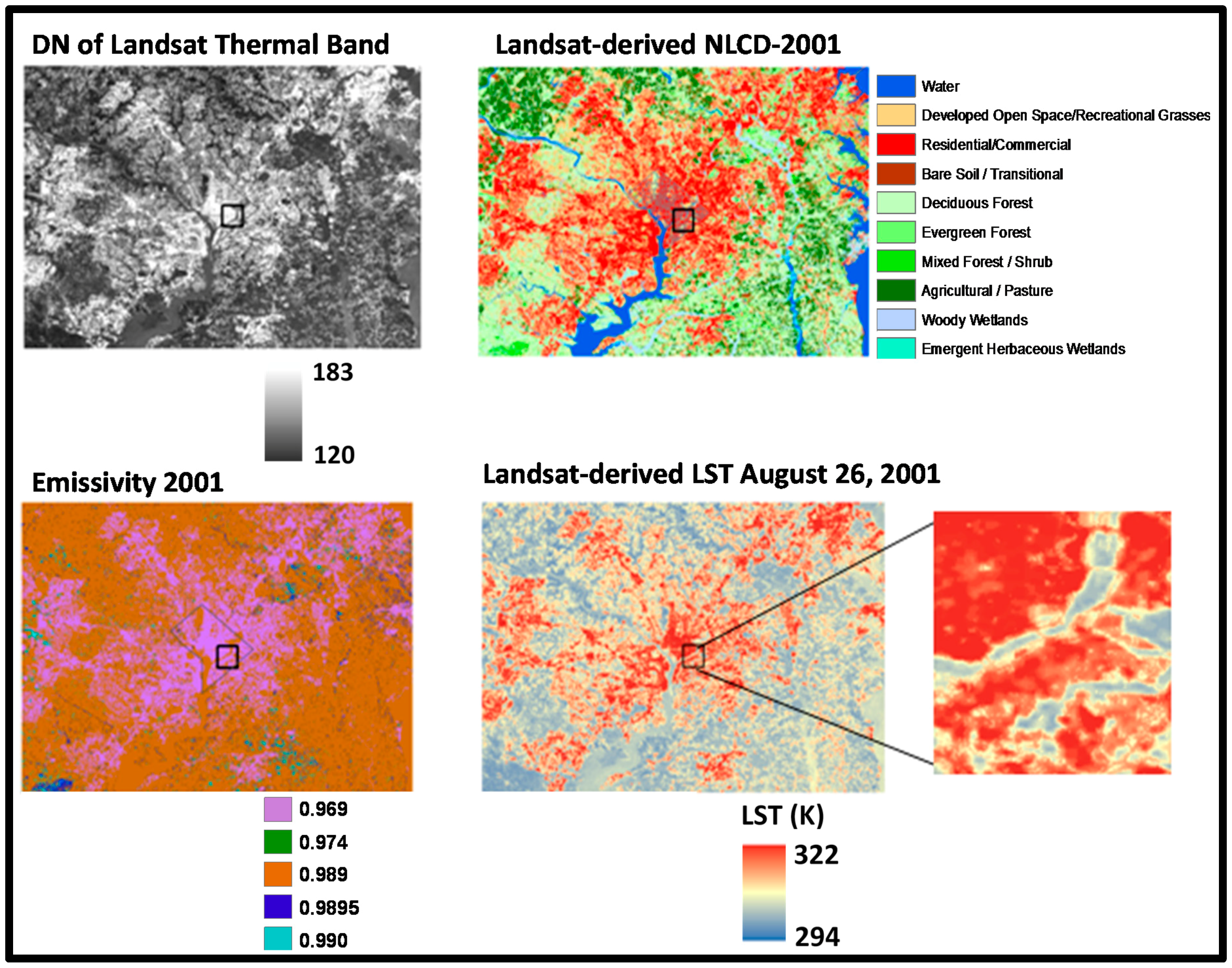
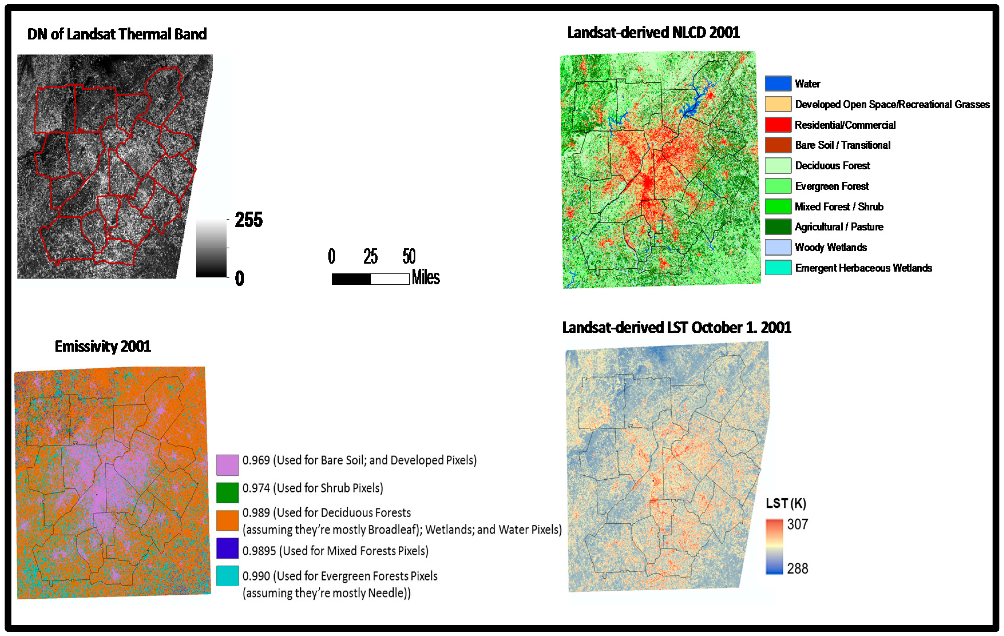
Examples of the raw Landsat data, NLCD-2001 LC data and emissivity data for Atlanta, New York, and Washington, which were used in deriving LST from the Landsat raw thermal imagery, and the resulting LST are shown in Figure 2, Figure 3 and Figure 4 respectively. Again, the locations of the two 5 km × 5 km cells (Cell 1 and Cell 2) in Atlanta, GA, two 5 km × 5 km cells (Cell 1 and Cell 2) in New York, NY, and one 5 km × 5 km cell in Washington, DC, where these analyses were performed are all shown in Figure 1.

5. Results and Discussion

5.1. SiB2 Sensitivity to Emissivity

The emissivity is a key factor in land surface temperature measurements. However, most climate and land surface models conventionally set this parameter as a constant. In the Simple Biosphere model (SiB2) the emissivity is set to 1 for all land cover types.

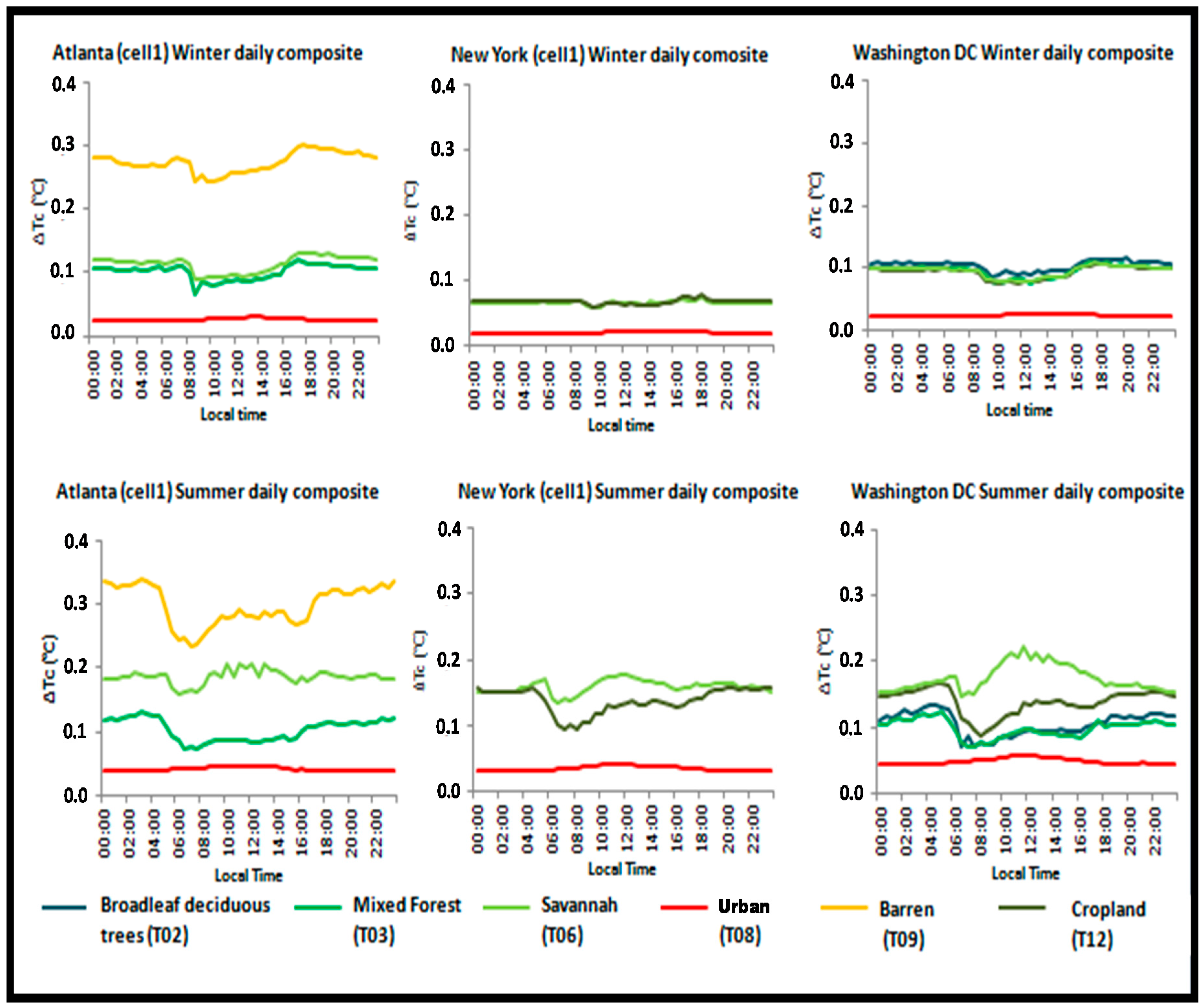
Sensitivity analyses were conducted to examine the impact of variable surface emissivity on the SiB2 simulated canopy temperature (TC). In Figure 5, we present the seasonal mean differences ∆Tc in the daily composite canopy temperatures simulated by SiB2 using constant emissivity (scenario SiB_Fr) and land cover type-dependent emissivites (scenario SiB_FrEm) (∆Tc = TC (SiB_FrEm) − TC (SiB_Fr)). The results illustrate that the assumption of the constant emissivity induces small error in modeling the canopy temperature over the studied points. The highest errors occur over bare land, with changes up to 0.34 °C in summer daily composite canopy temperature. This change is slightly less important during the winter time and the daily variation shows a minimal impact during the daytime. It is recognized that emissivity is an important parameter in the modeling of the surface energy balance and is difficult to measure. It varies with the state of the land surface itself, depending on surface weather conditions.

5.2. Comparison of SiB2 Canopy Temperature to Landsat and MODIS-Derived LST

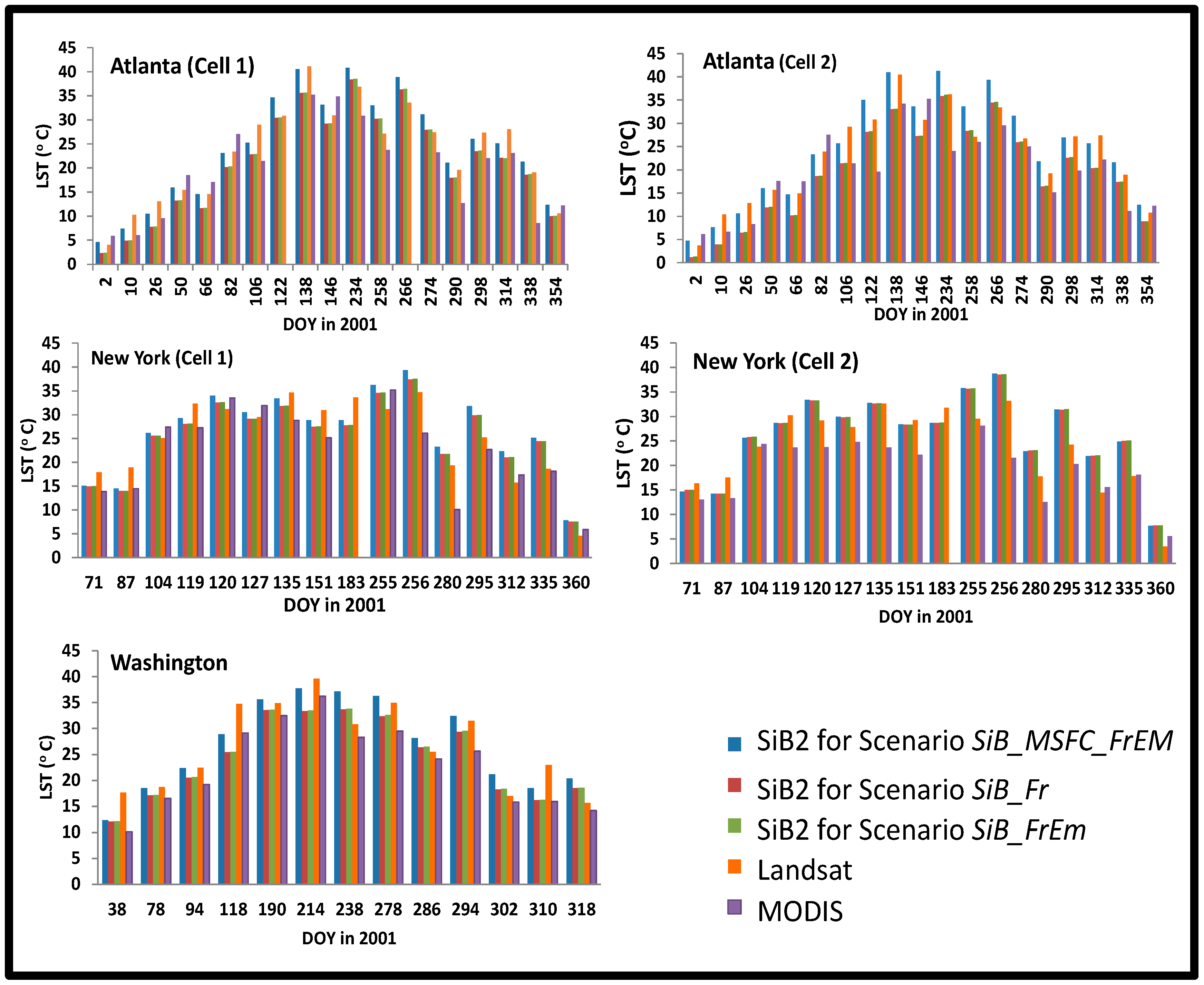
The results (time series) of all of the SiB2 LST model runs of the three scenarios are described above in Section 4.1 (SiB_Fr, SiB_FrEm, SiB_MSFC_FrEM), Landsat-derived LST and MODIS LST for all of the studied points and days are shown in Figure 6. It is very obvious that all of the datasets have similar trends in general, despite the differences in magnitude. Thus, in order to evaluate the sensitivity of the SiB2 LST to different LC types/fractions and emissivities compared to the same baseline/reference points derived from Landsat thermal data, root mean square difference (RMSD), mean difference (MD), and correlation coefficient (R) statistics were computed for each SiB2 model scenario and shown in

Table 3. Root mean square difference (RMSD) (compared to Landsat), mean difference (MD), and R statistics for all SiB2 model LST and MODIS LST compared to all Landsat-derived LST data.

Model/Statistic	RMSD	RMSD	RMSD	RMSD	RMSD
	(R)	(R)	(R)	(R)	(R)
	(MD)	(MD)	(MD)	(MD)	(MD)
Location	Atlanta-Cell 1	Atlanta-Cell 2	NY-Cell 1	NY-Cell 2	DC-Cell 1
MODIS_LST	11.53	5.80	9.56	8.69	4.36
	(0.90)	(0.86)	(0.88)	(0.90)	(0.96)
	(−5.80)	(−3.17)	(−4.11)	(−5.53)	(−3.80)
SiB2 for Scenario SiB_Fr	3.46	4.46	3.74	4.12	4.31
	(0.97)	(0.96)	(0.89)	(0.89)	(0.89)
	(−2.05)	(−3.55)	(0.26)	(2.54)	(−2.29)
SiB2 for Scenario SiB_FrEm	3.43	4.39	3.75	4.15	4.27
	(0.97)	(0.96)	(0.89)	(0.89)	(0.89)
	(−1.99)	(−3.43)	(0.32)	(2.59)	(−2.18)
SiB2 for Scenario SiB_MSFC_FrEM	2.92	3.24	4.18	4.13	3.69
	(0.97)	(0.97)	(0.89)	(0.90)	(0.90)
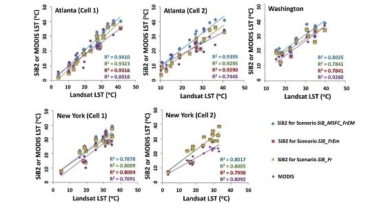
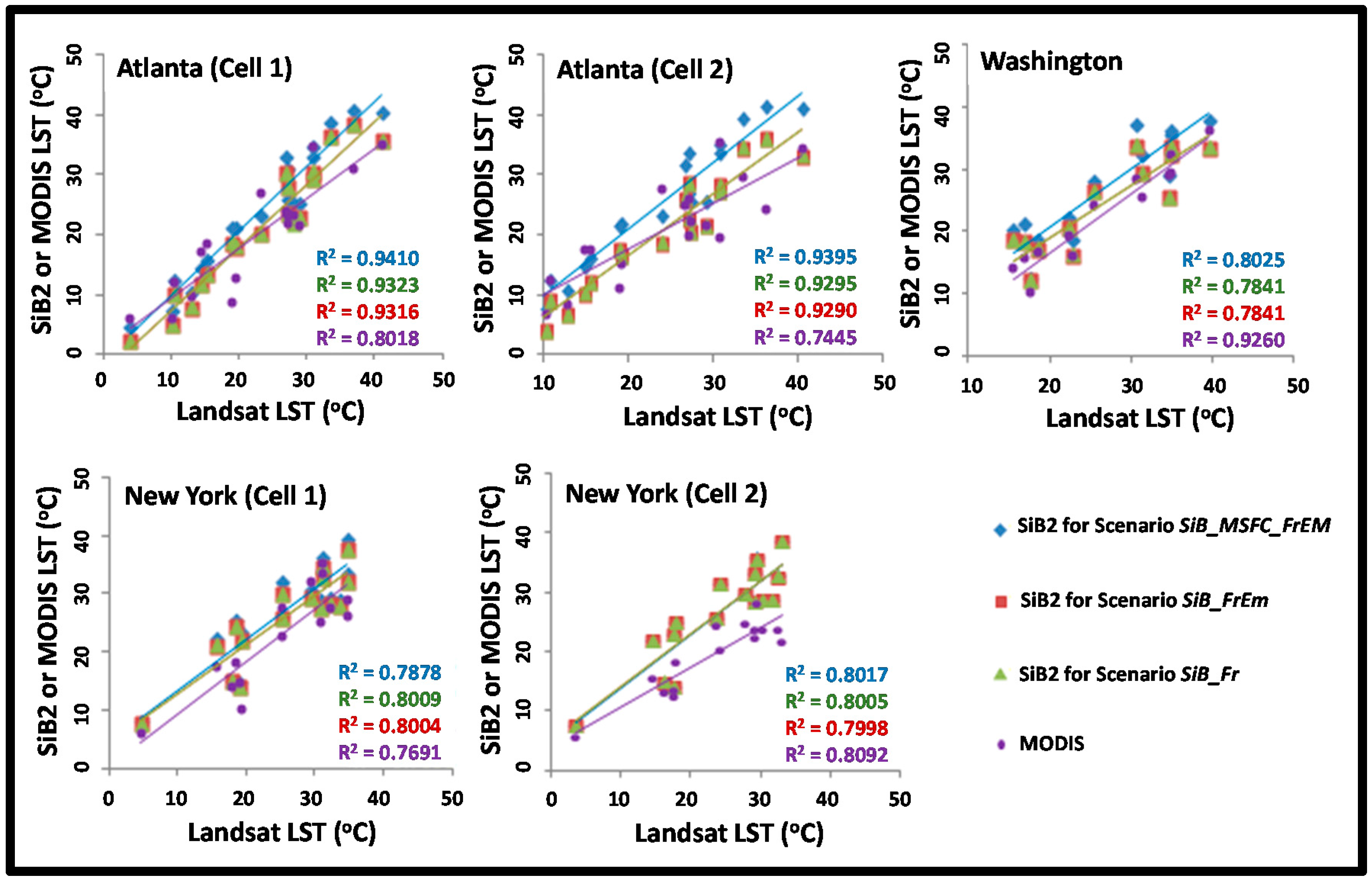
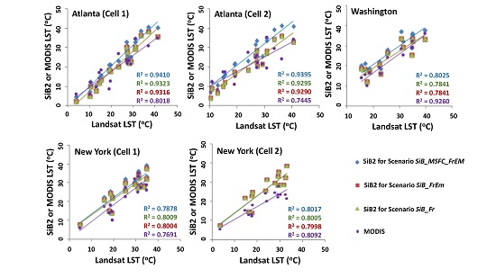
	(0.91)	(1.42)	(1.45)	(2.55)	(0.23)

. Scatterplots were generated and shown in Figure 7. We have also compared the Landsat-derived LST to MODIS LST to see whether the SiB2 or MODIS LST is more similar to the Landsat-derived LST, and those results are also included in Figure 6 and Figure 7 and Table 3 as well.

Our results have shown that, in general, using detailed emissivities per different LC type instead of a constant value of 1.0 for all LC types slightly reduced the differences between SiB2 and Landsat-derived LST. This change in emissivities generally reduced the RMSD by only 0.9%–1.6% in Atlanta and Washington, while it barely changed in New York. These slight differences could be due to the fact that while it is a more accurate representation of reality to use the detailed emissivity per LC type, the emissivities ranged from 0.969 to 0.989 (with many LC types of 0.989), so it is still close in magnitude to 1.0 within all of the areas.

As shown in Table 3 and Figure 6, our results have shown that using the NLCD LC type fractions instead of the NLCD ISA generally, and more significantly, reduced the differences between the SiB2 LST and Landsat LST in Atlanta and Washington, where the urban NLCD LC type is 71%–74% and ISA is 21%–43%, respectively. The reduction in RMSD when only LC fractions were changed was much larger than only emissivities were changed (RMSD reduction of 13.6%–26.2% vs. 0.9%–1.6%). Thus, this LC fractions change of using the NLCD LC type fractions instead of the NLCD ISA further closed the gap between SiB2 LST and Landsat LST by 13.6%–26.2% making it a total RMSD reduction of 14.5%–27.8%. On the other hand, using the NLCD LC type fractions increased the differences between the SiB2 LST and Landsat LST in New York, where the urban NLCD LC type is 91%–99% and ISA is 71%–82%. The reason for these opposite results in Atlanta and Washington versus New York could be due to the following: The NLCD residential/commercial developed classes are defined as areas with a mixture of constructed materials and vegetation, whose impervious surfaces account for 20%–49%, 50%–79%, or 80%–100% for low-intensity, medium-intensity, or high-intensity developed classes, respectively. Once the NLCD LC is defined, it becomes a nominal class and the whole area that fits that criterion is assigned to that class. Thus, in Scenario 3 of the SiB2 model run, we aggregated all of the residential/commercial classes into one and the summed percentage was entered into the SiB2 model as the urban/built up class, which are all considered as impervious surfaces in the SiB2 model. In the case of the New York grid cells, while the percentage of the nominal urban/buildup class was 91%–99%, it is a large overestimation to consider it all as an impervious surface, which also causes an overestimation in the LST values that are evident in the high positive MD in New York. Our results have also shown that, in general, SiB2 model LST data are closer in magnitude to the Landsat-derived LST than the MODIS LST data are to the Landsat-derived LST. Furthermore, as clearly shown in Figure 7, our results have shown strong linear relationships between the SiB2 model LST (of all scenarios) and the Landsat LST with linear correlation coefficients of 0.89–0.99, as well as the MODIS LST and Landsat LST with linear correlation coefficients of 0.83–0.99.

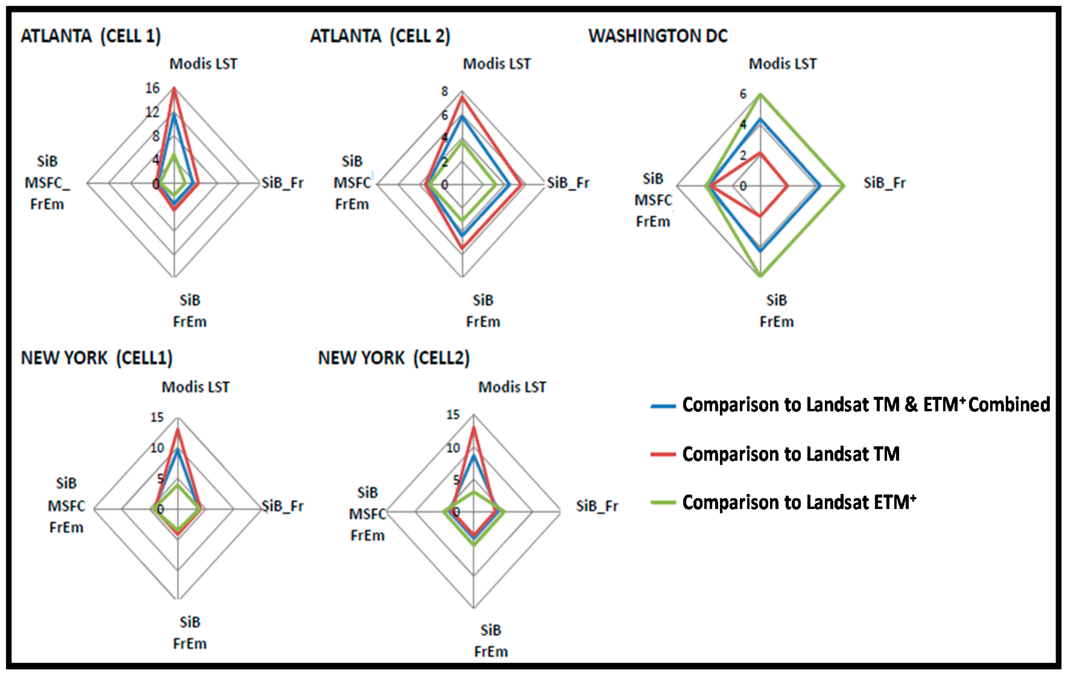
In order to see whether there are differences in the results/analysis between the Landsat 5 TM and Landsat 7 ETM⁺ data, we have also computed the RMSD, MD, and R statistics separately for their respective datasets (

Table 4. RMSD, MD, and R statistics for SiB2 model LST and MODIS LST compared only to Landsat 5 TM-derived LST.

Model/Statistic	RMSD	RMSD	RMSD	RMSD	RMSD
	(R)	(R)	(R)	(R)	(R)
	(MD)	(MD)	(MD)	(MD)	(MD)
Location	Atlanta-Cell 1	Atlanta-Cell 2	NY-Cell 1	NY-Cell 2	DC-Cell 1
MODIS_LST	15.95	7.49	12.94	13.05	2.16
	(0.99)	(0.95)	(0.97)	(0.95)	(0.99)
	(−11.30)	(−6.90)	(−8.75)	(−9.68)	(−2.05)
SiB2 for Scenario SiB_Fr	4.53	5.56	4.10	3.64	1.95
	(0.97)	(0.97)	(0.89)	(0.89)	(0.96)
	(−3.12)	(−4.65)	(−2.12)	(0.28)	(0.42)
SiB2 for Scenario SiB_FrEm	4.50	5.47	4.08	3.66	1.99
	(0.96)	(0.96)	(0.89)	(0.89)	(0.96)
	(−3.06)	(−4.52)	(−2.07)	(0.33)	(0.52)
SiB2 for Scenario SiB_MSFC_FrEM	3.28	3.45	4.04	3.69	3.53
	(0.97)	(0.97)	(0.88)	(0.89)	(0.94)
	(0.08)	(0.57)	(−0.90)	(0.30)	(2.61)

and

Table 5. RMSD, MD, and R statistics for SiB2 model LST and MODIS LST compared only to Landsat 7 ETM⁺-derived LST.

Model/Statistic	RMSD	RMSD	RMSD	RMSD	RMSD
	(R)	(R)	(R)	(R)	(R)
	(MD)	(MD)	(MD)	(MD)	(MD)
Location	Atlanta-Cell 1	Atlanta-Cell 2	NY-Cell 1	NY-Cell 2	DC-Cell 1
MODIS_LST	4.87	3.65	3.91	3.04	5.98
	(0.83)	(0.90)	(0.94)	(0.95)	(0.99)
	(−0.84)	(0.20)	(0.52)	(−1.38)	(−5.83)
SiB2 for Scenario SiB_Fr	2.07	3.17	3.34	5.20	5.99
	(0.98)	(0.98)	(0.97)	(0.97)	(0.95)
	(−1.09)	(−2.56)	(2.65)	(4.80)	(−5.45)
SiB2 for Scenario SiB_FrEm	2.04	3.09	3.39	5.25	5.91
	(0.98)	(0.98)	(0.97)	(0.97)	(0.95)
	(−1.02)	(−2.46)	(2.70)	(4.86)	(−5.33)
SiB2 for Scenario SiB_MSFC_FrEM	2.55	3.05	4.32	5.17	3.86
	(0.99)	(0.98)	(0.97)	(0.97)	(0.96)
	(1.81)	(2.19)	(3.80)	(4.79)	(−2.55)

and Figure 8). Our results have also shown that SiB2 LST is generally closer in magnitude to Landsat 5 TM-derived LST than it is to Landsat 7 ETM⁺-derived LST in New York and Washington, but the opposite is true in Atlanta. It is important to emphasize here that none of the remote sensing data are direct observations but rather modeled LSTs and, as such, do not represent a ground truth. SiB2 is a biophysical model that has attempted to describe the urban metabolism and includes uncertainties that may or may not be of the same size as those related to the retrievals of emissivities and LST from remote sensing.

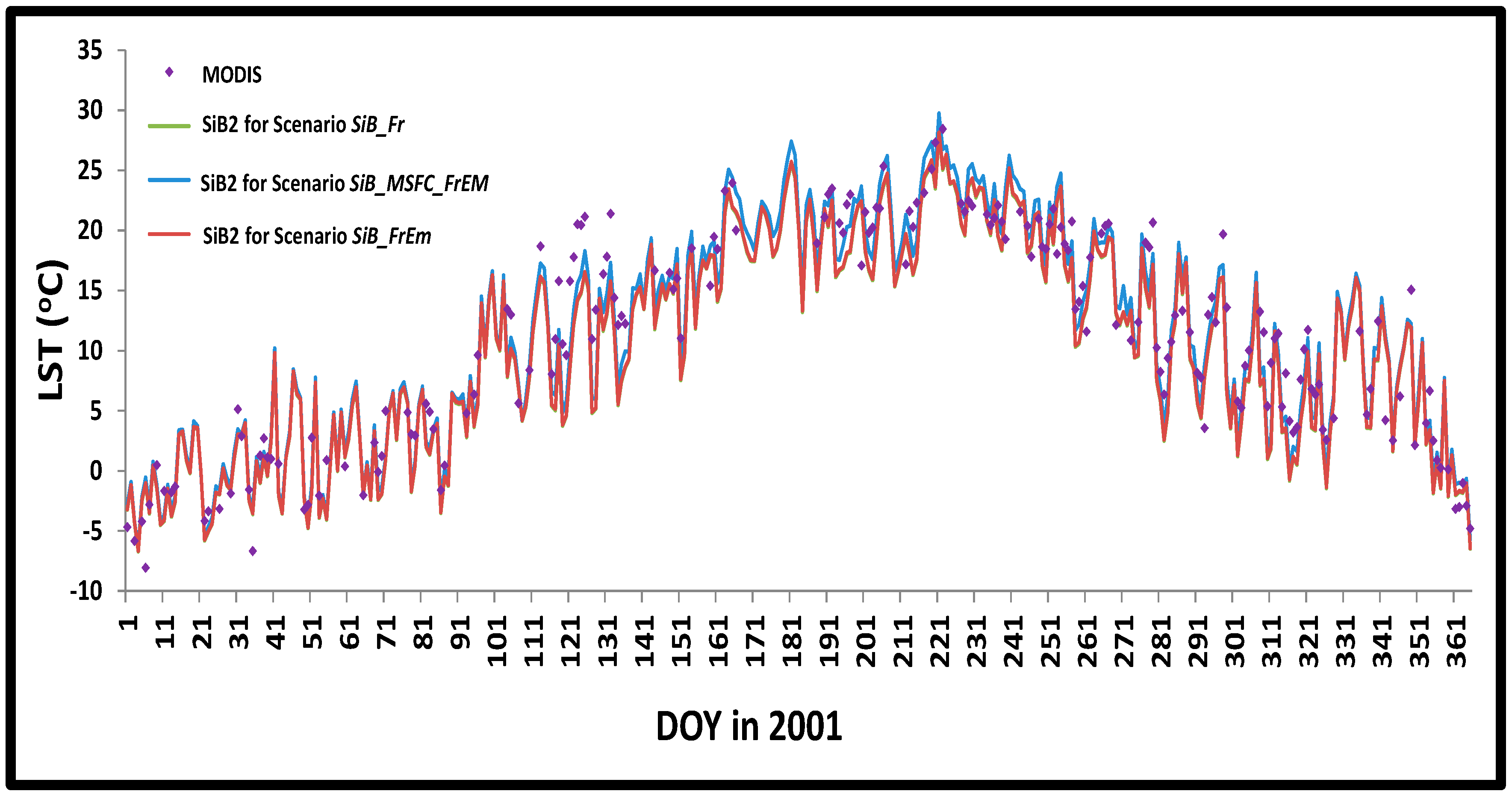
As mentioned before, all of the previously-discussed analyses were performed using daytime LST data in this comparison study due to the Landsat overpass time, which ranges from 10:30 am–noon local time over our study areas. However, we also performed additional analyses where we compared nighttime SiB2 model simulated canopy temperature to MODIS nighttime LST, which showed smaller differences in LST and less sensitivity to land cover composition than those of daytime LST as demonstrated for Washington, DC, in Figure 9 and

Table 6. Root mean square difference (RMSD) and mean difference (MD) for nighttime and daytime SiB2 model simulated canopy temperature compared to MODIS nighttime and daytime LST, respectively, for the 5 km × 5 km cell in Washington, DC.

Model	SiB2 for Scenario SiB_Fr		SiB2 for Scenario SiB_FrEm		SiB2 for Scenario SiB_MSFC_FrEM
Time/Statistic	RMSD	MD	RMSD	MD	RMSD	MD
Nighttime	3.26	1.90	3.20	1.80	2.69	0.82
Daytime	4.45	−3.17	4.55	−3.28	6.36	−5.33

.

5.3. Land Surface Temperature Sensitivity to Land Cover Type

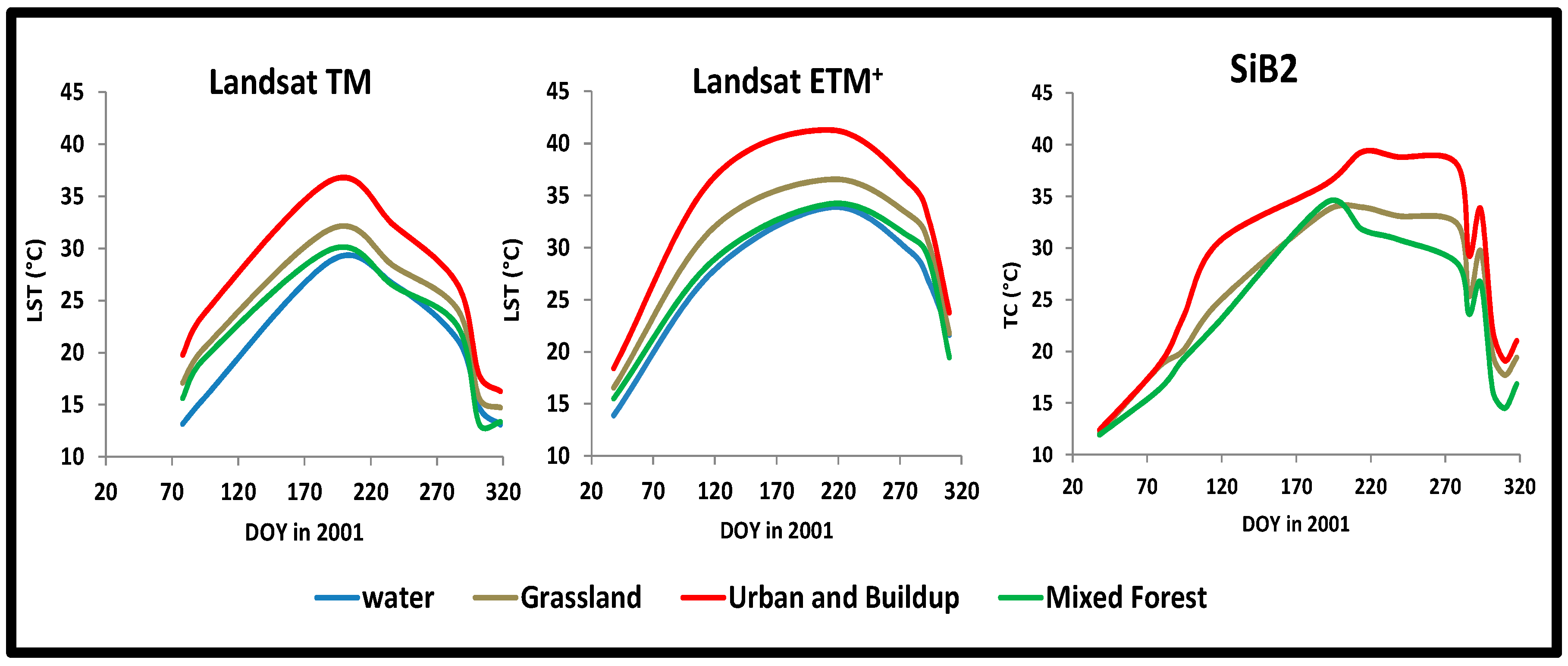
Further analyses were performed to assess temperature differences in urban areas, and to evaluate and compare the relationship between urban surface temperature and land cover types for SiB2 and Landsat. Our results (Figure 10) over Washington, DC, showed that land surface temperature is related to land cover type. For both data, impervious area has the greatest temperature, followed by grassland, then forest, which makes physical sense given the cooling that takes place in vegetated surfaces due to the evapotranspiration (ET) process. In addition, since trees can use their deep root systems to access more soil moisture than grasses, forested areas had lower surface temperatures than grasslands.

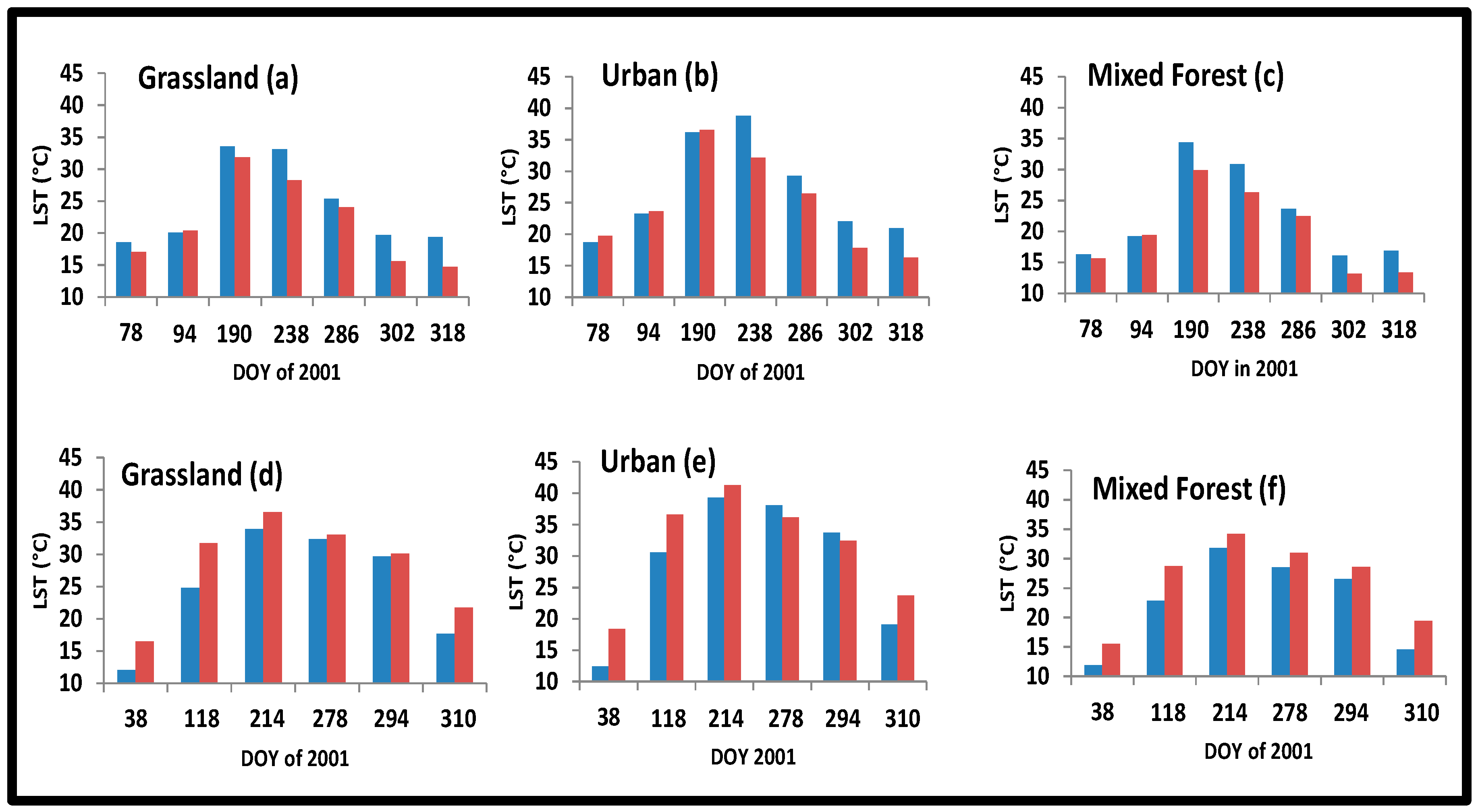
A comparison of SiB2 canopy temperature to Landsat TM and ETM⁺-derived LST for each land cover was conducted (Figure 11). Results show that for all land cover types over the Washington, DC, 5 km × 5 km cell, SiB2 canopy temperature is slightly higher than Landsat TM-derived LST and cooler than Landsat ETM⁺-derived LST.

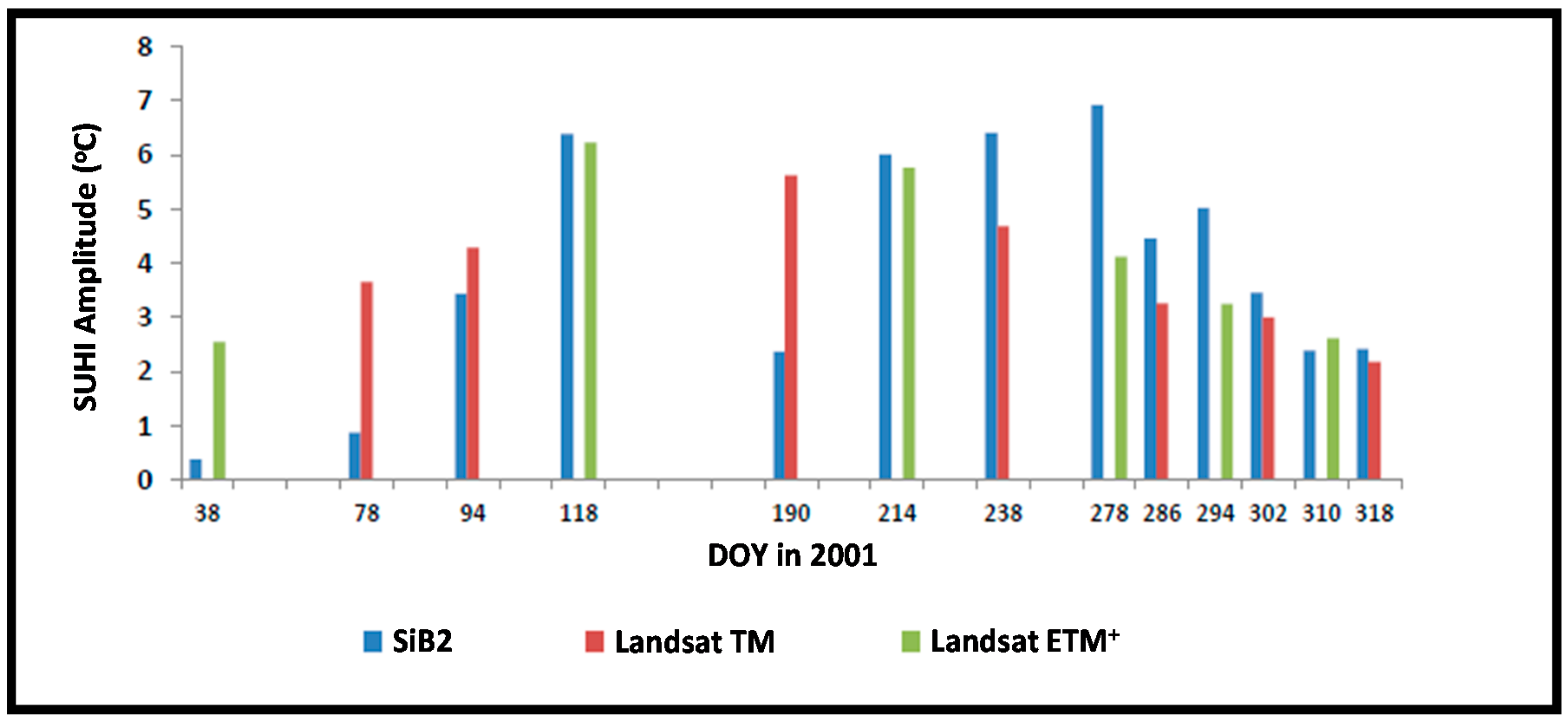
We also analyzed the surface urban heat island (SUHI) amplitude, defined as difference in land surface temperature (LST) between the ISA and the vegetated land surrounding it, and compared the results for SiB2, Landsat TM, and ETM⁺ (Figure 12). Results for the Washington, DC, cell show that Landsat ETM⁺ sensed the highest average SUHI amplitude (4.09 °C), followed by SiB2 (3.89 °C), and Landsat TM (3.81 °C). The RMSD has been computed to Landsat TM- and ETM⁺-sensed SUHI amplitudes, in comparison to the SiB2 simulated SUHI amplitude (

Table 7. Average, RMSD, and MD statistics for Landsat TM and ETM⁺ SUHI amplitude in comparison to SiB2 SUHI amplitude.

	SiB2	Landsat TM	Landsat ETM+
Average SUHI amplitude (°C)	3.89	3.81	4.09
Mean difference in SUHI amplitude compared to SiB2 (°C)		−0.47	0.87
RMSD in SUHI amplitude compared to SiB2 (°C)		1.85	1.89

), which shows that both sensors have the same RMSD as compared to SiB2.

6. Summary and Conclusions

The main aim of this study was to evaluate the land surface temperature (LST) in urban centers, and for that we used two different approaches: one by using purely remote sensing, and the other by using physical modeling assimilated with remotely-sensed data. Thus, a fusion of Landsat and MODIS data, along with SiB2 model data, were used in this study to assess the impact of different land cover (LC) types/fractions and emissivity on LST and the urban heat island phenomenon in selected cities. To that end, we evaluated the sensitivity of the SiB2 LST to different LC types/fractions and emissivities compared to the same baseline/reference point derived from Landsat thermal data. This evaluation was demonstrated in three climatologically- and morphologically-different cities of Atlanta, GA, New York, NY, and Washington, DC. Our results showed that, in these study areas, the SiB2 model was sensitive to both emissivity and LC types/fractions, but much more sensitive to the latter. The practical implications of these results are rather significant since they imply that the SiB2 model can be used to run different scenarios for detecting and forecasting SUHI for current and future potential LC changes and for evaluating urban heat island mitigation strategies.

This study also showed that using detailed emissivities per different LC type, instead of a constant value of 1.0 for all LC types, closes the gap slightly between SiB2 LST and Landsat-derived LST. In addition, this study also showed that using the NLCD LC type fractions instead of the NLCD ISA for running the SiB2 model generally closes the gap further between SiB2 LST and Landsat-derived LST, except for very highly urbanized cities, such as New York, where the urban NLCD LC type is 91%–99% and ISA is 71%–82%. In other words, using detailed emissivities per LC type and LC fractions from Landsat-derived NLCD generally caused a convergence of the model results towards the Landsat-derived LST for most of the cases in this study. Furthermore, this study also showed that SiB2 model LST data are generally closer in magnitude to Landsat-derived LST than MODIS LST data are to Landsat-derived LST. However, it is important to reemphasize here that none of the remote sensing data are direct observations but rather modeled LSTs and, as such, do not represent a ground truth, so more studies will be needed in the future to compare these results to in situ LST data and provide further validation.

References

- Li, Z.L.; Tang, B.H.; Wu, H.; Ren, H.; Yan, G.; Wan, Z.; Sobrino, J.A. Satellite-derived land surface temperature: Current status and perspectives. Remote Sens. Environ. 2013, 131, 14–37. [Google Scholar] [CrossRef]
- Imhoff, M.L.; Zhang, P.; Wolfe, R.E.; Bounoua, L. Remote sensing of the urban heat island effect across biomes in the continental USA. Remote Sens. Environ. 2010, 114, 504–513. [Google Scholar] [CrossRef]
- Anderson, M.C.; Norman, J.M.; Kustas, W.P.; Houborg, R.; Starks, P.J.; Agam, N. A thermal-based remote sensing technique for routine mapping of land-surface carbon, water and energy fluxes from field to regional scales. Remote Sens. Environ. 2008, 112, 4227–4241. [Google Scholar] [CrossRef]
- Sellers, P.J.; Randall, D.A.; Collatz, G.J.; Berry, J.A.; Field, C.B.; Dazlich, D.A.; Zhang, C.; Bounoua, L. A revised land surface parameterization (SiB2) for atmospheric GCMs. Part I: Model formulation. J. Clim. 1996, 9, 676–705. [Google Scholar] [CrossRef]
- Bounoua, L.; Safia, A.; Masek, J.; Peters-Lidard, C.; Imhoff, M.L. Impact of Urban Growth on Surface Climate: A Case Study in Oran, Algeria. J. Clim. Appl. Meteorol. 2009, 48, 217–231. [Google Scholar] [CrossRef]
- Jin, M.; Liang, S. An Improved Land Surface Emissivity Parameter for Land Surface Models Using Global Remote Sensing Observations. J. Clim. 2006, 19, 2867–2881. [Google Scholar] [CrossRef]
- Wenny, B.N.; Xiong, X.; Madhavan, S.; Wu, A.; Li, Y. Long-term band-to-band calibration stability of MODIS thermal emissive bands. In Proceedings of the SPIE Defense, Security, and Sensing 2013, Baltimore, MD, USA, 29 April–3 May 2013.
- Price, J.C. Land surface temperature measurements from the split window channels of the NOAA-7 AVHRR. J. Geophys. Res. 1984, 79, 5039–5044. [Google Scholar]
- Wan, Z.; Dozier, J. A generalized split-window algorithm for retrieving land-surface temperature from space. IEEE Trans. Geosci. Remote Sens. 1996, 34, 892–905. [Google Scholar]
- Thome, K.J. Absolute radiometric calibration of Landsat 7 ETM+ using the reflectance-based model. Remote Sens. Environ. 2001, 78, 27–38. [Google Scholar] [CrossRef]
- Sobrino, J.A.; Jimenez-Munoz, J.C.; Paolina, L. Land surface temperature retrieval from LANDSAT TM 5. Remote Sens. Environ. 2004, 90, 434–440. [Google Scholar] [CrossRef]
- Al-Hamdan, M.Z.; Crosson, W.L.; Estes, M.G.; Estes, S.M.; Quattrochi, D.A.; Johnson, D.P. Downscaling MODIS Land Surface Temperature Using Landsat-derived Data. 2016; in preparation. [Google Scholar]
- Xiao, R.B.; Ouyang, Z.Y.; Zheng, H.; Li, W.F.; Schienke, E.W.; Wang, X.K. Spatial pattern of impervious surfaces and their impacts on land surface temperature in Beijing, China. J. Environ. Sci. 2007, 19, 250–256. [Google Scholar] [CrossRef]
- Suga, Y.; Ogaw, H.; Ohno, K.; Yamada, K. Detection of Surface Temperature from Landsat-7/ETM+. Adv. Space Res. 2003, 32, 2235–2240. [Google Scholar] [CrossRef]
- Weng, Q.H.; Lu, D.S.; Schubring, J. Estimation of land surface temperature-vegetation abundance relationship for urban heat island studies. Remote Sens. Environ. 2004, 89, 467–483. [Google Scholar] [CrossRef]
- Weng, Q.; Lu, D.; Liang, B. Urban surface biophysical descriptors and land surface temperature variations. Photogramm. Eng. Remote Sens. 2006, 72, 1275–1286. [Google Scholar] [CrossRef]
- Weng, Q.; Liu, H.; Lu, D. Assessing the effects of land use and land cover patterns on thermal conditions using landscape metrics in city of Indianapolis, United States. Urban Ecosyst. 2007, 10, 203–219. [Google Scholar] [CrossRef]
- Bounoua, L.; Zhang, P.; Safia, A.; Masek, J.; Imhoff, M.; Thome, K.; Wolfe, R.E. Mapping biophysical parameters for land surface modeling over the continental US using MODIS and landsat. Dataset Pap. Sci. 2015, 2015, 564279. [Google Scholar] [CrossRef]
- Bounoua, L.; Zhang, P.; Mostovoy, G.; Thome, K.; Masek, J.; Imhoff, M.; Shepherd, M.; Quattrochi, D.; Santanello, J.; Silva, J.; et al. Impact of urbanization on US surface climate. Environ. Res. Lett. 2015, 10, 84010–84018. [Google Scholar] [CrossRef]
- Homer, C.; Dewitz, J.; Fry, J.; Coan, M.; Hossain, N.; Larson, C.; Herold, N.; McKerrow, A.; VanDriel, J.N.; Wickham, J. Completion of the 2001 National Land Cover Database for the Conterminous United States. Photogramm. Eng. Remote Sens. 2007, 73, 337–341. [Google Scholar]
- Snyder, W.C.; Wan, Z.; Zhang, Y.; Feng, Y.Z. Classification based emissivity for land surface temperature measurement from space. Int. J. Remote Sens. 1998, 19, 2753–2774. [Google Scholar] [CrossRef]
- Artis, D.A.; Carnahan, W.H. Survey of emissivity variability in thermography of urban areas. Remote Sens. Environ. 1982, 12, 313–329. [Google Scholar] [CrossRef]
Figure 1.
The spatial domains of the study areas (5 km × 5 km cells) and NLCD-2001 LC within those areas.
Figure 2.
An example of Landsat-derived LST for Atlanta on 1 October 2001 and inputs needed for that derivation.
Figure 3.
An example of Landsat-derived LST for New York on 14 April 2001 and inputs needed for that derivation.
Figure 4.
An example of Landsat-derived LST for Washington, DC on 26 August 2001 and inputs needed for that derivation (the extracted block represents the 5 km × 5 km cell where analyses were performed).
Figure 5.
Differences in daily composite of canopy temperature computed with Landcover type-dependent emissivity and constant emissivity. Results are averaged during winter (December, January, and February) and summer (June, July and August).
Figure 6.
Time series of LST results from all SiB2 model scenarios, Landsat, and MODIS for Atlanta, Washington, DC, and New York.
Figure 7.
Landsat LST versus MODIS LST or SiB2 LST for Atlanta, Washington, DC, and New York.
Figure 8.
Root mean square difference (RMSD) between Landsat thermal data (TM, ETM+, and TM and ETM+ combined), each SiB2 model scenario, and MODIS.
Figure 9.
Comparison of nighttime SiB2 simulated canopy temperature for each model scenario and MODIS nighttime LST for the 5 km × 5 km cell in Washington, DC.
Figure 10.
Landsat TM- and ETM+-derived land surface temperatures and SiB2 canopy temperature for each land cover type present in the 5 km × 5 km cell in Washington, DC.
Figure 11.
Comparison of SiB2 canopy temperature (blue) to Landsat TM (a–c) and ETM+ (d–f) LST (red) for each land cover type in the 5 km × 5 km cell in Washington, DC.
Figure 12.
SUHI amplitude computed using SiB2 Canopy temperature, Landsat TM- and Landsat ETM+-derived LST over the 5 km × 5 km cell in Washington, DC.