
Regionalization of Uncovered Agricultural Soils Based on Organic Carbon and Soil Texture Estimations

Abstract
:1. Introduction
2. Materials and Methods
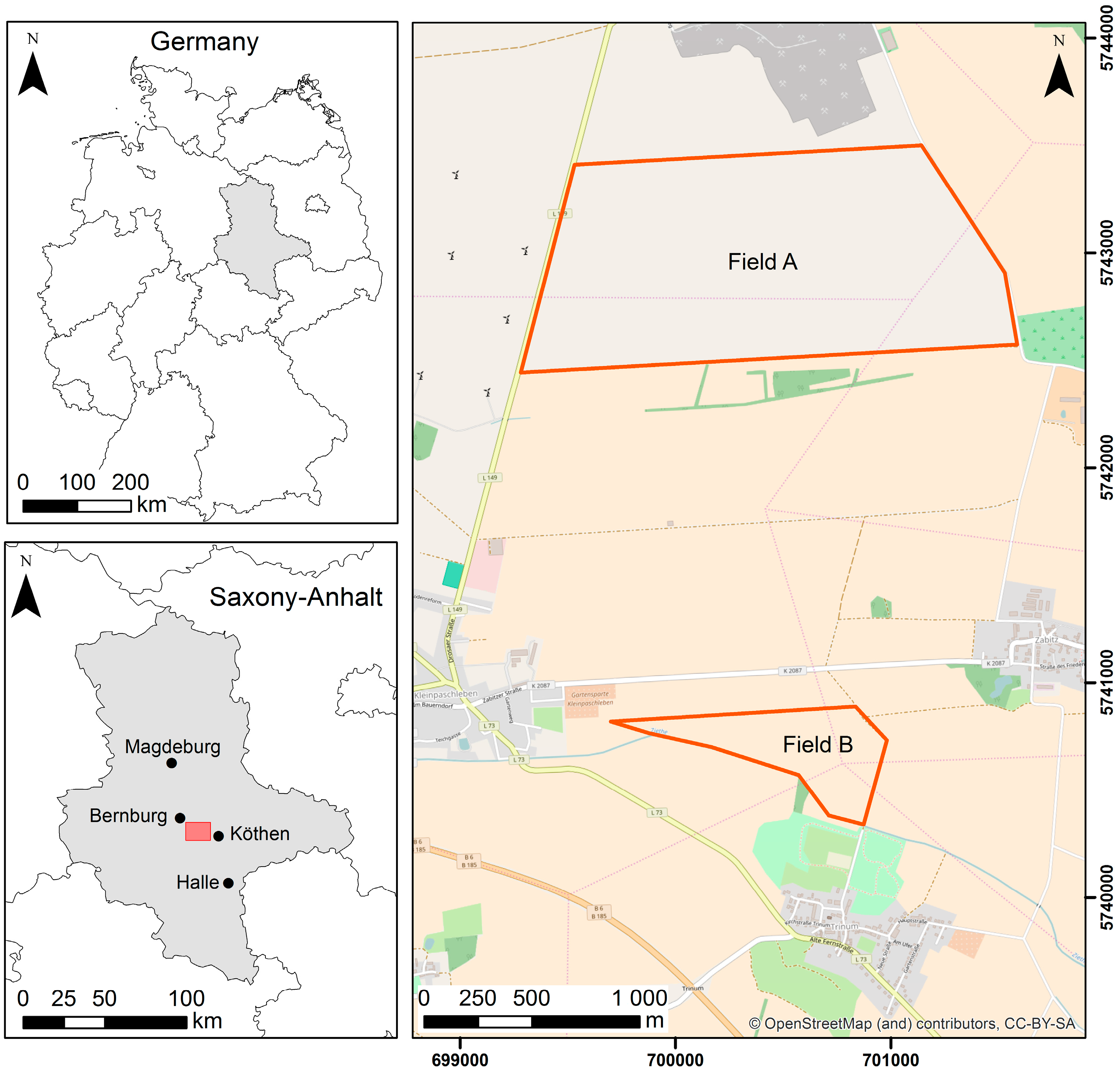
2.1. Study Area
2.2. Data and Preprocessing
2.2.1. Laboratory Data
2.2.2. Airborne Data
2.3. Methodology
3. Results
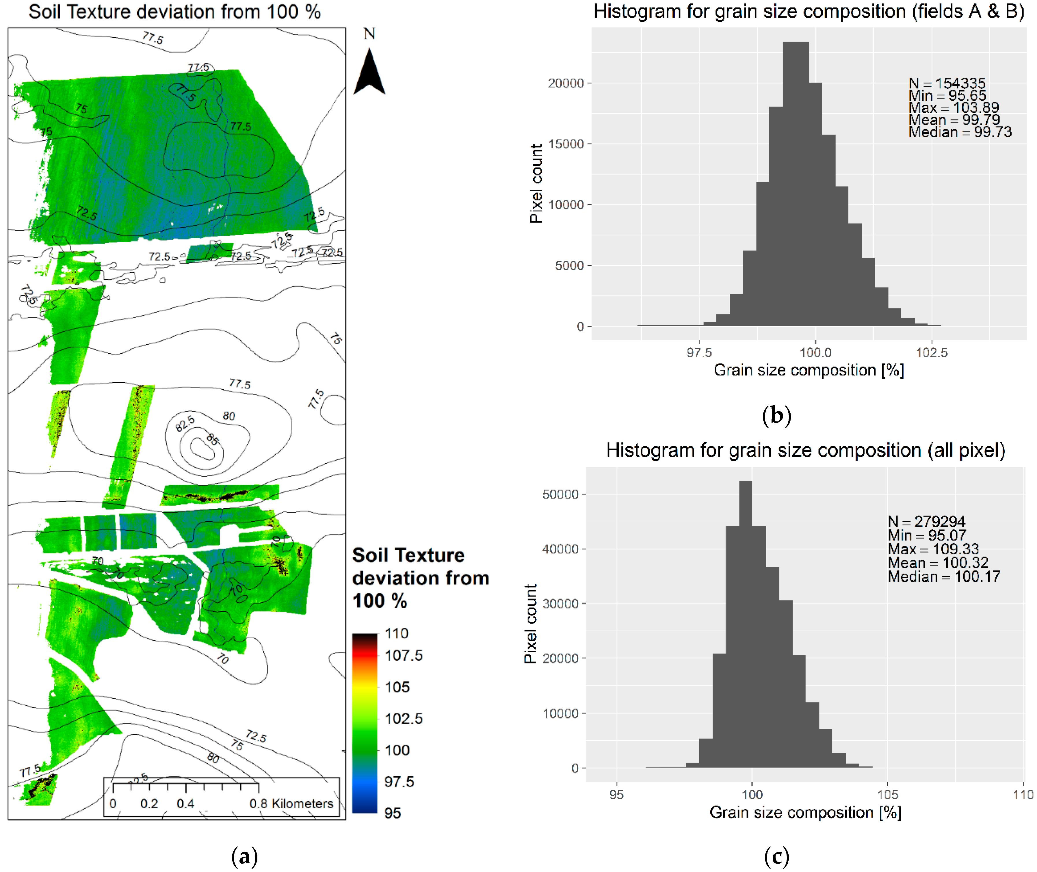
3.1. Data Analysis
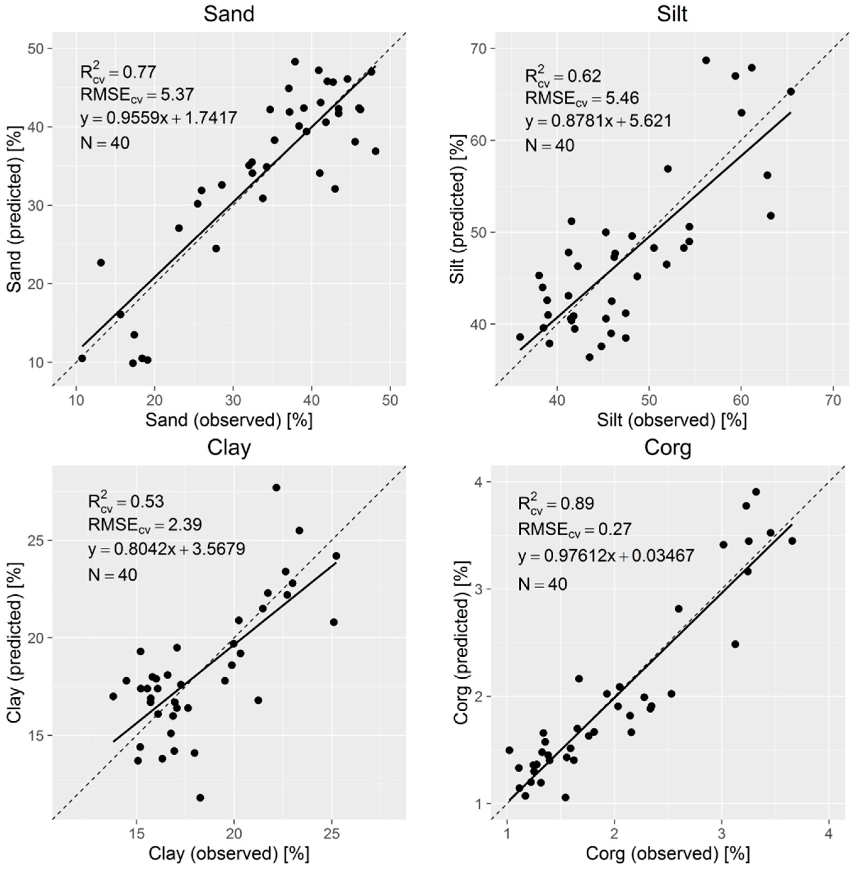
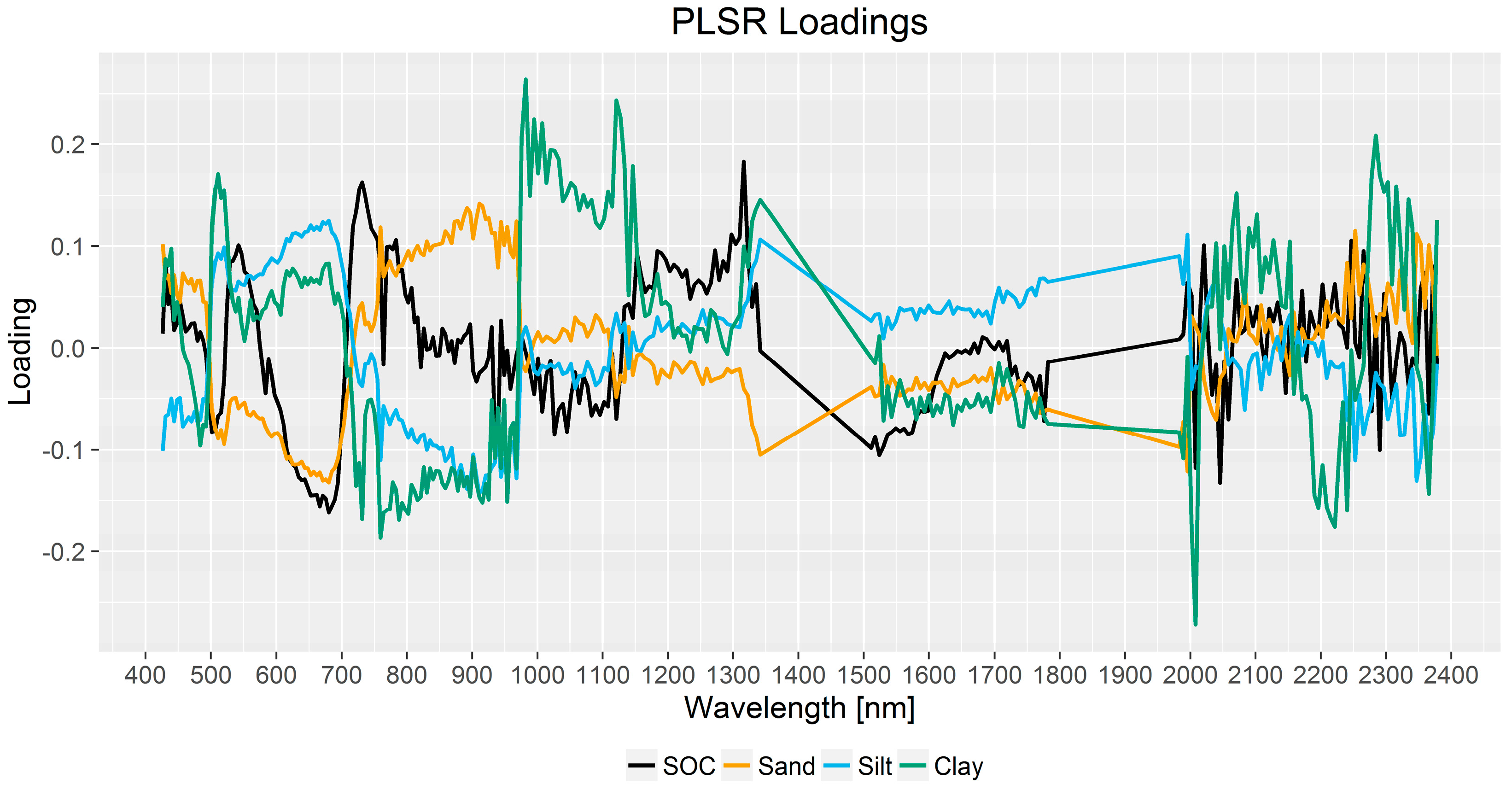
3.2. PLSR
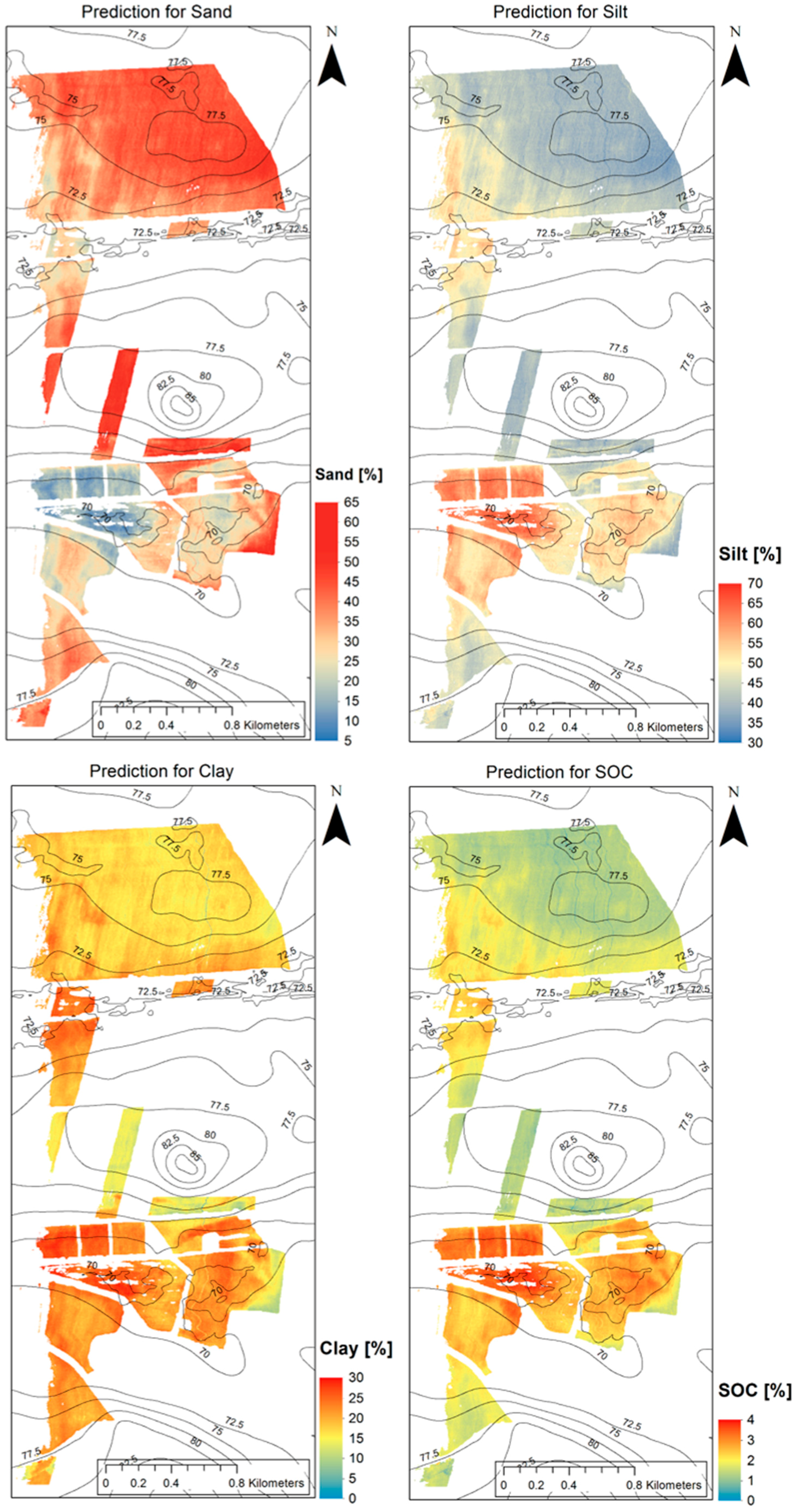
3.3. Classification/Regionalization
4. Discussion
5. Conclusions
Acknowledgments
Author Contributions
Conflicts of Interest
References
- Food and Agriculture Organization of the United Nations (FAO). World Soil Charter. 2015. Available online: http://www.fao.org/3/a-mn442e.pdf (accessed on 17 December 2015).
- Food and Agriculture Organization of the United Nations (FAO). Status of the World’s Soil Resources. 2015. Available online: http://www.fao.org/3/a-i5199e.pdf (accessed on 17 December 2015).
- Gebbers, R.; Adamchuk, V.I. Precision agriculture and food security. Science 2010, 327, 828–831. [Google Scholar] [CrossRef] [PubMed]
- Adamchuk, V.I.; Hummel, J.W.; Morgan, M.T.; Upadhyaya, S.K. On-the-go soil sensors for precision agriculture. Comput. Electron. Agric. 2004, 44, 71–91. [Google Scholar] [CrossRef]
- Adhikari, K.; Hartemink, A.E.; Minasny, B.; Bou Kheir, R.; Greve, M.B.; Greve, M.H. Digital mapping of soil organic carbon contents and stocks in Denmark. PLoS ONE 2014, 9, e105519. [Google Scholar] [CrossRef] [PubMed]
- Grimm, R.; Behrens, T.; Märker, M.; Elsenbeer, A. Soil organic carbon concentrations and stocks on Barro Colorado Island—Digital soil mapping using random forests analysis. Geoderma 2008, 146, 102–113. [Google Scholar] [CrossRef]
- De Brogniez, D.; Ballabio, C.; Stevens, A.; Jones, R.J.A.; Montanarella, L.; van Wesemael, B. A Map of the topsoil organic carbon content of Europe generated by a generalized additive model. Eur. J. Soil Sci. 2015, 66, 121–134. [Google Scholar] [CrossRef]
- Villa, P.; Malucelli, F.; Scalenghe, R. Carbon Stocks in Peri-Urban Areas: A case study of remote sensing capabilities. IEEE J. Sel. Top. Appl. Earth Obs. Remote Sens. 2014, 7, 4119–4128. [Google Scholar] [CrossRef]
- Peralta, N.R.; Costa, J.L.; Balzarini, M.; Angelini, H. Delineation of management zones with measurements of soil apparent electrical conductivity in the southeastern Pampas. Can. J. Soil Sci. 2013, 93, 205–218. [Google Scholar] [CrossRef]
- Mulder, V.L.; de Bruin, S.; Schaepman, M.E.; Mayr, T.R. The Use of Remote sensing in soil and terrain mapping—A review. Geoderma 2011, 162, 1–19. [Google Scholar] [CrossRef]
- Blume, H.-P.; Brümmer, G.; Horn, R.; Kandeler, E.; Kögel-Knabner, I.; Kretzschmar, R.; Stahr, K.; Wilke, B.-M. Scheffer/Schachtschabel Lehrbuch der Bodenkunde, 16th ed.; Spektrum Akademischer Verlag: Heidelberg, Germany, 2010. [Google Scholar]
- Minasny, B.; McBratney, A.B. Digital soil mapping—A brief history and some lessons. Geoderma 2016, 264, 301–311. [Google Scholar] [CrossRef]
- Nanni, M.R.; Demattê, J.A.M. Spectral reflectance methodology in comparison to traditional soil analysis. Soil Sci. Soc. Am. J. 2006, 70, 393–407. [Google Scholar] [CrossRef]
- Demattê, J.A.M.; Fiorio, P.R.; Araújo, S.R. Variation of routine soil analysis when compared with hyperspectral narrow band sensing method. Remote Sens. 2010, 2, 1998–2016. [Google Scholar] [CrossRef]
- Demattê, J.A.M.; Alves, M.R.; Gallo, B.C.; Fongaro, C.T.; e Souza, A.B.; Romero, D.J.; Sato, M.V. Hyperspectral remote sensing as an alternative to estimate soil attributes. Revista Ciência Agronômica 2015, 46, 223–232. [Google Scholar] [CrossRef]
- Casa, R.; Castaldi, F.; Pascucci, S.; Palombo, A.; Pignatti, S. A Comparison of sensor resolution and calibration strategies for soil texture estimation from hyperspectral remote sensing. Geoderma 2013, 197–198, 17–26. [Google Scholar] [CrossRef]
- Chang, C.-W.; Laird, D.; Mausbach, M.J.; Hurburgh, C.R. Near-infrared reflectance spectroscopy—Principal components regression analyses of soil properties. Soil Sci. Soc. Am. J. 2001, 65, 480–490. [Google Scholar] [CrossRef]
- Selige, T.; Böhner, J.; Schmidhalter, U. High resolution topsoil mapping using hyperspectral image and field data in multivariate regression modeling procedures. Geoderma 2006, 136, 235–244. [Google Scholar] [CrossRef]
- Gomez, C.; Lagacherie, P.; Coulouma, G. Regional predictions of eight common soil properties and their spatial structures from hyperspectral Vis-NIR data. Geoderma 2012, 189–190, 176–185. [Google Scholar] [CrossRef]
- Hively, W.D.; McCarty, G.W.; Reeves, J.B., III; Lang, M.W.; Oesterling, R.A.; Delwiche, S.R. Use of airborne hyperspectral imagery to map soil properties in tilled agricultural fields. Appl. Environ. Soil Sci. 2011. [Google Scholar] [CrossRef]
- Reeves, D.W. The role of soil organic matter in maintaining soil quality in continuous cropping systems. Soil Tillage Res. 1997, 43, 131–167. [Google Scholar] [CrossRef]
- Shatar, T.M.; McBratney, A.B. Empirical modelling of relationships between sorghum yield and soil properties. Precis. Agric. 1999, 1, 249–276. [Google Scholar] [CrossRef]
- Ladoni, M.; Bahrami, H.A.; Alavipanah, S.K.; Norouzi, A.A. Estimating soil organic carbon from soil reflectance—A review. Precis. Agric. 2010, 11, 82–99. [Google Scholar] [CrossRef]
- Patzold, S.; Mertens, F.M.; Bornemann, L.; Koleczek, B.; Franke, J.; Feilhauer, H.; Welp, G. Soil heterogeneity at the field scale—A challenge for precision crop protection. Prec. Agric. 2008, 9, 367–390. [Google Scholar] [CrossRef]
- McCarty, G.W.; Reeves, J.B., III; Reeves, V.B.; Follett, R.F.; Kimble, J.M. Mid-infrared and near-infrared diffuse reflectance spectroscopy for soil carbon measurements. Soil Sci. Soc. Am. J. 2002, 66, 640–646. [Google Scholar]
- Rossel, R.A.; Walvoort, D.J.J.; McBratney, A.B.; Janik, L.J.; Skjemsta, J.O. Visible, near infrared, mid infrared or combined diffuse reflectance spectroscopy for simultaneous assessment of various soil properties. Geoderma 2006, 131, 59–75. [Google Scholar] [CrossRef]
- Jarmer, T.; Vohland, M.; Lilienthal, H.; Schnug, E. Estimation of some chemical properties of an agricultural soil by spectroradiometric measurements. Pedosphere 2008, 18, 163–170. [Google Scholar] [CrossRef]
- Stevens, A.; Udelhoven, T.; Denis, A.; Tychon, B.; Lioy, R.; Hoffmann, L.; van Wesemael, B. Measuring soil organic carbon in croplands at regional scale using airborne imaging spectroscopy. Geoderma 2010, 158, 32–45. [Google Scholar] [CrossRef]
- Schwanghart, W.; Jarmer, T. Linking spatial patterns of soil organic carbon to topography—A case study from south-eastern Spain. Geomorphology 2011, 126, 252–263. [Google Scholar] [CrossRef]
- Gomez, C.; Viscarra Rossel, R.A.; McBratney, A.B. Soil organic carbon prediction by hyperspectral remote sensing and field Vis-NIR spectroscopy—An Australian case study. Geoderma 2008, 146, 403–411. [Google Scholar] [CrossRef]
- Jarmer, T.; Hill, J.; Lavée, H.; Sarah, P. Mapping Topsoil organic carbon in non-agricultural semi-arid and arid ecosystems of Israel. Photogramm. Eng. Remote Sens. 2010, 75, 85–94. [Google Scholar] [CrossRef]
- Deutscher Wetterdienst. Climate Data Center. Available online: ftp://ftp-cdc.dwd.de/pub/CDC/observations_germany/climate/monthly/kl/historical/ (accessed on 22 April 2016).
- European Commission and the European Soil Bureau Network. The European Soil Database Distribution Version 2.0; CD-ROM, EUR 19945 EN; European Commission: Brussels, Belgium; European Soil Bureau Network: Ispra, Italy, 2004. [Google Scholar]
- Food and Agriculture Organization of the United Nations (FAO); IUSS Working Group WRB. World Reference Base for Soil Resources 2014 (Update 2015) International Soil Classification System for Naming Soils and Creating Legends for Soil Maps; World Soil Resources Reports, No. 106; FAO: Rome, Italy, 2015. [Google Scholar]
- International Organization of Standardization (ISO). 11277:2009 Soil Quality—Determination of Particle Size Distribution in Mineral Soil Material—Method by Sieving and Sedimentation; International Organization of Standardization (ISO): Geneva, Switzerland, 2009. [Google Scholar]
- Deutsches Institut für Normung e.V. (DIN). Soil—Investigation and Testing—Determination of Ignition Loss; 18128:2002-12; Deutsches Institut für Normung e.V. (DIN): Coblenz, Germany, 2002. [Google Scholar]
- Rogaß, C.; Spengler, D.; Bochow, M.; Segl, K.; Lausch, A.; Doktor, D.; Roessner, S.; Behling, R.; Wetzel, H.U.; Kaufmann, H. Reduction of Radiometric miscalibration—Application to pushbroom sensors. Sensors 2011, 11, 6370–6395. [Google Scholar] [CrossRef] [PubMed]
- Rouse, J.W.; Haas, R.H.; Schell, J.A.; Deering, D.W. Monitoring vegetation systems in the Great Plains with ERTS. In Proceedings of the Third Earth Resources Technology Satellite-1 Symposium, Washington, DC, USA, 10–14 December 1973; Volume 1, pp. 309–317.
- Price, J.C. Estimating leaf area index from satellite data. IEEE Trans. Geosci. Remote Sens. 1993, 31, 727–734. [Google Scholar] [CrossRef]
- Mevik, B.-H.; Wehrens, R.; Liland, K.H. pls: Partial least squares and principal component regression. R package Version 2.5-0. 2015. Available online: https://CRAN.R-project.org/package=pls (accessed on 21 April 2016).
- Sinowski, W.; Auerswald, K. Using relief parameters in a discriminant analysis to stratify geological areas with different spatial variability of soil properties. Geoderma 1999, 89, 113–128. [Google Scholar] [CrossRef]
- Moore, I.D.; Gessler, P.E.; Nielsen, G.A.; Peterson, G.A. Soil attribute prediction using terrain analysis. Soil Sci. Soci. Am. J. 1993, 57, 443–452. [Google Scholar] [CrossRef]
- Lyles, L.; Tatarko, J. Wind erosion effects on soil texture and organic matter. J. Soil Water Conserv. 1986, 41, 191–193. [Google Scholar]


| Sensor | Method | R2 Sand [%] | R2 Silt [%] | R2 Clay [%] | R2 SOC [%] | Reference |
|---|---|---|---|---|---|---|
| Laboratory | ||||||
| IRIS | MR | 0.79 | 0.27 | 0.91 | 0.80 | [13] |
| IRIS | MR | 0.82 | 0.57 | 0.86 | 0.30 | [14] |
| ASD | PLSR | 0.79 | 0.63 | 0.58 | - | [16] |
| ASD | PLSR | - | - | - | 0.93 | [24] |
| ASD | PLSR | - | - | - | 0.62 | [27] |
| NIRSystems | PCR | 0.82 | 0.82 | 0.67 | - | [17] |
| NIRSystems | PLSR | - | - | - | 0.98 | [25] |
| Varian Cary 500 | PLSR | 0.75 | 0.52 | 0.67 | 0.72 | [26] |
| Airborne/Spaceborne Imagery | ||||||
| HyMap | PLSR | 0.95 | - | 0.71 | 0.90 | [18] |
| HyMap | PLSR | 0.20 | 0.17 | 0.67 | 0.02 | [19] |
| HyMap | PLSR | - | - | - | 0.77 | [29] |
| HyperSpecTIR | PLSR | 0.79 | 0.79 | 0.66 | 0.65 | [20] |
| AHS | PSR | - | - | - | 0.75 | [28] |
| Landsat TM | MR | 0.53 | - | 0.68 | 0.51 | [13] |
| Landsat TM | MR | 0.64 | 0.54 | 0.61 | 0.41 | [14] |
| Landsat TM | PLSR | - | - | - | 0.91 | [31] |
| Hyperion | PLSR | - | - | - | 0.51 | [30] |
| Parameter | n | Min. | Max. | Mean | SD |
|---|---|---|---|---|---|
| Sand [%] (0.063–2 mm) | 40 | 9.9 | 48.3 | 34.3 | 11.4 |
| Silt [%] (2–63 µm) | 40 | 36.4 | 68.7 | 47.4 | 8.9 |
| Clay [%] (<2 µm) | 40 | 11.8 | 27.7 | 18.3 | 3.4 |
| SOC [%] | 40 | 1.06 | 3.91 | 1.97 | 0.82 |
| Height [m] | 40 | 69.85 | 78.24 | 73.89 | 2.69 |
| Sand | Height | Clay | Silt | SOC | |
|---|---|---|---|---|---|
| Sand | 1 | 0.82 | −0.81 | −0.97 | −0.94 |
| Height | - | 1 | −0.67 | −0.81 | −0.85 |
| Clay | - | - | 1 | 0.66 | 0.80 |
| Silt | - | - | - | 1 | 0.90 |
| SOC | - | - | - | - | 1 |
© 2016 by the authors; licensee MDPI, Basel, Switzerland. This article is an open access article distributed under the terms and conditions of the Creative Commons Attribution (CC-BY) license (http://creativecommons.org/licenses/by/4.0/).
Share and Cite
Kanning, M.; Siegmann, B.; Jarmer, T. Regionalization of Uncovered Agricultural Soils Based on Organic Carbon and Soil Texture Estimations. Remote Sens. 2016, 8, 927. https://doi.org/10.3390/rs8110927
Kanning M, Siegmann B, Jarmer T. Regionalization of Uncovered Agricultural Soils Based on Organic Carbon and Soil Texture Estimations. Remote Sensing. 2016; 8(11):927. https://doi.org/10.3390/rs8110927
Chicago/Turabian StyleKanning, Martin, Bastian Siegmann, and Thomas Jarmer. 2016. "Regionalization of Uncovered Agricultural Soils Based on Organic Carbon and Soil Texture Estimations" Remote Sensing 8, no. 11: 927. https://doi.org/10.3390/rs8110927