1. Introduction
Riparian ecotones, transition zones between water and land, provide a variety of important ecosystem functions and services. The range extends from filtering/buffering of sediment and nutrient load to stream bank stabilization, from water storage/release to aquifer recharge, and from habitat provision to recreational and educational opportunities [
1,
2,
3,
4]. Riparian zones are considered exceptionally rich in biodiversity [
5,
6] and extremely fragile at the same time [
7]. Despite its high ecological value, a large part of the natural riparian vegetation has already been lost, degraded or fragmented due to human activity [
8,
9].
To counteract further riparian decline, initiatives at several scales have been put in place. At a global scale, the Millennium Ecosystem Assessment requests measures for systematic assessment of riverine habitats [
1]. The EU Biodiversity Strategy to 2020 addresses the issue at European policy level, aiming to halt the loss of biodiversity and the degradation of ecosystem services in the EU by 2020, restoring them as far as feasible [
10]. The EU Biodiversity strategy’s target 2 focus is on a better protection and restoration of ecosystems and the services they provide, and greater use of green infrastructure,
sensu Benedict and McMahon [
11]. As a consequence, Copernicus (previously known as GMES, Global Monitoring for Environment and Security), the European flagship initiative for Earth Observation and Monitoring, is addressing these ecologically important areas. As part of the Copernicus Land Monitoring Service’s local component, “riparian zones” have been mapped during the Copernicus Initial Operations 2011–2013 phase on request of the European Environment Agency (EEA). Local component products are designed to provide specific and more detailed information focusing on specific types of hotspots, in this case riparian zones. Moreover, the local component “riparian zones” is expected to support the MAES initiative (Mapping and Assessment of Ecosystems and their Services [
12]) and link to other European policy areas or initiatives such as the Water Framework Directive, the Habitats and Birds Directives with their centrepiece the Natura 2000 network, the Floods Directive and the European Commission’s Green Infrastructure strategy [
13,
14,
15,
16,
17,
18]. Furthermore, the Blueprint to safeguard Europe’s waters calls for “strengthened measures to help the EU protect its water resources and become more resource (including water) efficient” [
19], urging for measures such as the restoration of wetlands and floodplains to increase the take-up of natural water retention.
Lastly, the Intergovernmental Science-Policy Platform on Biodiversity and Ecosystem Services (IPBES,
www.ipbes.net) would certainly benefit from these new datasets of continental extent (including Turkey) in their assessments on the state of biodiversity and of the ecosystem services it provides to society, namely, for the European assessment.
The aim of Copernicus’ local component “riparian zones” is to provide information on spatial extent, distribution and land cover/land use characteristics of riparian zones, for future systematic assessment of freshwater ecosystems and riverine habitats.
Riparian definitions are conceptual and fuzzy [
20] and among scientists sometimes controversial. In the present study we consider as riparian zone, in general terms, transitional areas occurring along land and freshwater ecosystems, characterized by unique soil, hydrology and biotic conditions strongly influenced by the stream water [
3,
20]. The riparian zone encompasses the stream channel between the low and high water marks and that portion of the terrestrial landscape from the high water mark toward the uplands where vegetation may be influenced by elevated water tables or flooding and by the ability of the soils to hold water [
6,
21].
European riparian zones, following the definition of Naiman et al. [
3], have been mapped in the past by the European Commission’s Joint Research Centre (JRC) [
22,
23]. An enhanced version of this data set has been developed and employed for ecosystem service assessments of riparian buffer capacity for European rivers [
24,
25]. Both, original and refined versions are JRC products and represent the first pan-European maps of riparian areas. At that time, the best available data sources were used to create a consistent and harmonized European product. However, now, as the technological and methodological progress continues, several improved base products have become available, which allow the compilation of a more complete, accurate and detailed product. Moreover, there are new requirements based on policy requests, which call for advanced monitoring, such as change analysis of land use/land cover, ecosystem condition and delivery of ecosystem services, including habitat and biodiversity monitoring. A riparian data set of high quality and detail, based on scientifically sound approaches, is needed to satisfy these requests. The demanding requirements add complexity to such an endeavour, but do certainly guarantee a high utility of the product. In terms of area extent, the requested coverage is bound to the 33 member and the 6 cooperating countries of the EEA. In terms of scale, the product is of high detail. Based on multi-resolution and multi-source satellite imagery, the Minimum Mapping Unit (MMU) is 0.5 ha.
The goal of this work is to design a riparian zones delineation model of high scientific value, being consistent, transparent, open for further input and repeatable in time, and at the same time serving a multitude of environmental needs.
Apart from the JRC riparian zones map [
22,
23,
24,
25], another similar work has been conducted by the Centre for International Forestry Research (CIFOR) [
26], focusing on global tropical wetlands. On a local or regional extent, riparian zones modelling and mapping has been carried out frequently, with a variety of approaches relying on all kind of Earth Observation (EO) data of different scale [
27,
28,
29,
30,
31,
32,
33,
34]. In all cases, the technique had been based on remote sensing data, often relying on a geomorphic approach, considering the topography, and/or relying on the proximity to water and/or the identification of riparian vegetation and features. Scientific evidence of the drivers determining the width of the riparian zone is reported by Naiman and Décamps [
5], which are in general related to the size of the stream, the position of the stream within the drainage network, the hydrological regime, and the local geomorphology. The employed data sources for regional/local analyses are often of high spatial detail, sometimes based on LIDAR (Light Detection and Ranging) data [
35]. To date, for a continental endeavour of riparian zone modelling and mapping such spatially very detailed data are not yet available. However, this might change in future.
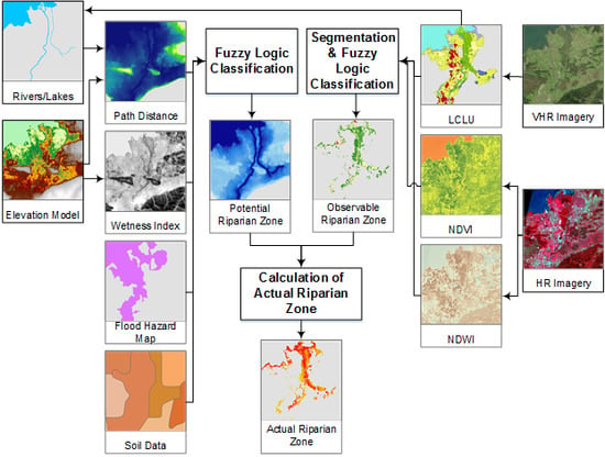
The general approach applied in this study is modular, whereby each module can be divided into several sub-modules. This way, the approach remains open for modifications, extensions, reductions or exchanges of modules or sub-modules. The design also ensures that riparian zones can still be modelled and mapped in case one or some input data sets are missing in a specific region. The main modules are organised such as to allow consecutive creation of “Potential Riparian Zones” (PRZ), mapping areas with a natural, physio-geographic disposition to host riparian zones; “Observable Riparian Zones” (ORZ) delineating effectively observed riparian zones; and “Actual Riparian Zones” (ARZ), representing the intersection of PRZ and ORZ.
PRZ are modelled based on the input features river network, terrain topography, soil properties, flood zones, modelled topographic wetness and the land cover/land use (LCLU) class “Water”. Following a fuzzy logic approach [
36], and an object based image analysis approach (OBIA) [
37], PRZ-specific membership (MS) values are assigned to segmented objects through a combination of feature-specific membership functions (MSFs). Regionalization/stratification is applied by assigning within each ECRINS river basin (European catchments and Rivers network system, see
Table 1) individual regional calibration factors when combining the input feature data.
The ORZ delineation relies mainly on satellite observations. The approach is analogous to the one of PRZ: MS values with respect to the input features LCLU, Normalized Difference Vegetation Index (NDVI) [
38], and Normalized Difference Water Index (NDWI) [
39] are combined.
PRZ and ORZ MSs are finally combined to the ARZ MS, expressing a probability to encounter riparian zones on ground. Eventually, applying a hard threshold to the raster based MS value, a vector-based delineation of riparian areas can be derived.
2. Materials and Methods
2.1. Study Site
Greater Europe is characterized by a high variety of bio-climatological regions or eco-regions [
40,
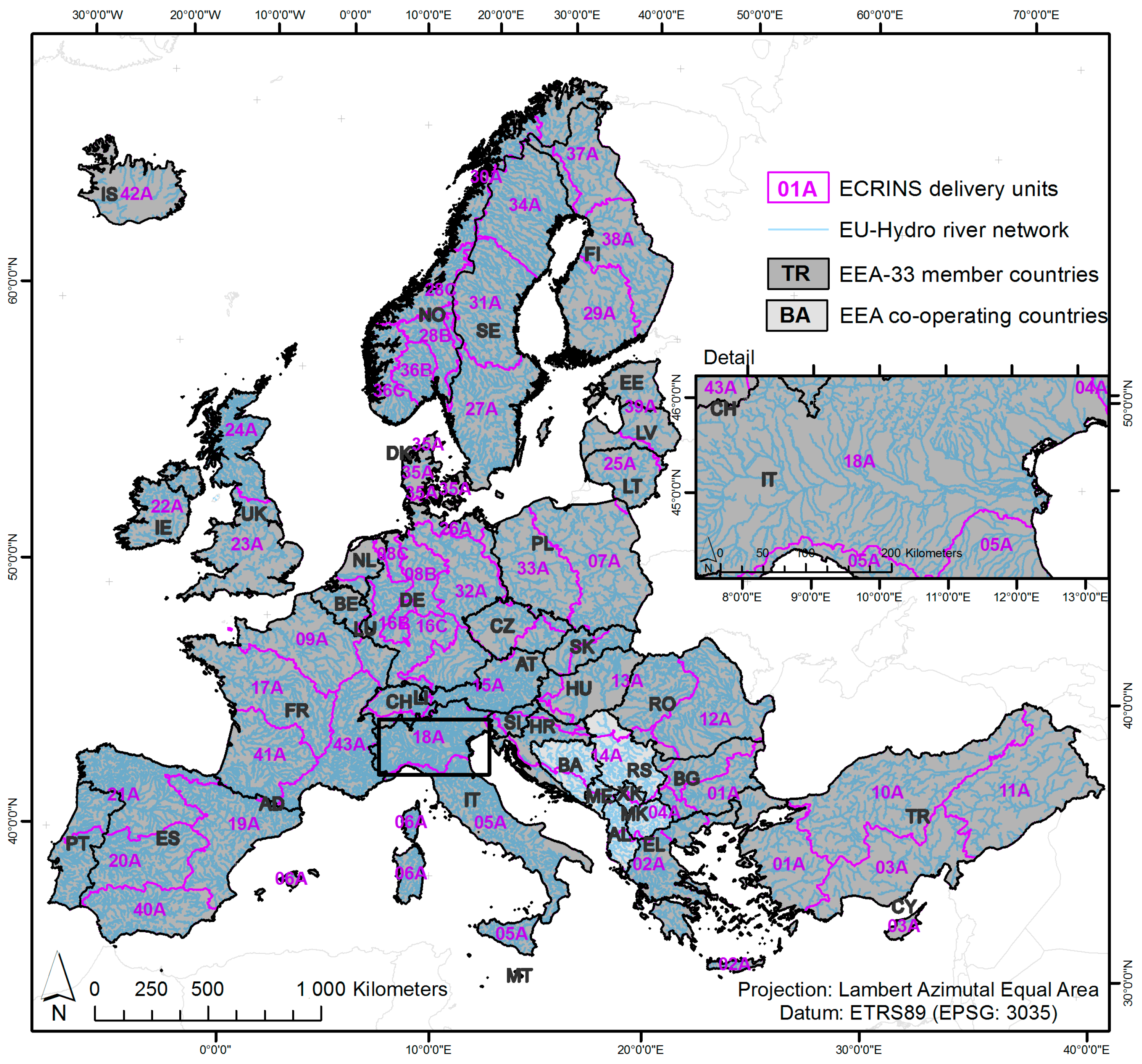
41]. This variety is even more pronounced if geological or soil data is being considered. For example, Europe’s most northern parts are considered arctic and boreal which contrast the Mediterranean or Turkey’s Anatolian regions. The extent of the study area ranges from 71.2°N to 34.6°S, and from 24.6°W to 44.9°E, comprising 33 member countries of the EEA and 6 cooperating countries (see
Figure 1). Besides all 28 EU member countries, also Iceland, Norway, Switzerland, Liechtenstein, Turkey and Albania, Bosnia and Herzegovina, Kosovo under the UN Security Council Resolution 1244/99, Former Yugoslav Republic of Macedonia, Montenegro and Serbia are covered. In addition, the small countries Andorra, San Marino and Vatican City are included.
The area of interest (AOI) of this study comprises an extended area of water influence around rivers and lakes: for a first delineation, based on the hydrological dataset EU-HYDRO, rivers of Strahler’s stream order 3–8 [
42] were selected and dynamic buffers built around them. The initial buffer widths were assumptions based on experience in previous studies [
22,
23], i.e., (to each river side) Strahler 3 + 4: 250 m, Strahler 5: 500 m, Strahler 6: 750 m, Strahler 7: 1000 m, Strahler 8: 1500 m. These initial areas were then combined with a flood hazard map which delineates the 100-year flood return period [
43]. The preliminary AOI extents to approx. 500,000 km
2 and is drained by a total river length of approximately 470,000 km. The river network comprises also lentic water bodies if one of the abovementioned selected rivers runs through them. This preliminary relatively coarse AOI has subsequently been expanded by approximately 10%, through adding additional, modelled PRZ area, as well as several additional relevant riparian areas and features (e.g., oxbow lakes of the relevant river systems) as visually identified in the Copernicus riparian zones LCLU dataset. Thus, the AOI comprises a total of 556,658 km
2.
2.2. Data
The riparian zones delineation model relies on data sets of different sources and scales, described hereafter and presented in
Table 1. The multi-scale approach makes it almost impossible to assign a common scale to the final product. However, to get a better understanding of this product’s scale, it might help to know some core characteristics of two crucial input datasets: the LCLU data set and the Digital Elevation Model (DEM). The Minimum Mapping Unit of the used LCLU data set is 0.5 ha, with an original spatial resolution of the underlying EO-input data ranging between 2 m (Pleiades) and 30 m (Landsat 8), whereas the applied EU-DEM has a spatial resolution of 25 m. Typically, the scales for these raster resolutions lie around 1:5000 (for 2 m) and 1:75,000 (for 30 m).
The data generally refers to the reference year 2012, with some exceptions or deviations, which in the case of quasi-static data (e.g., soil data) should not affect the result. All data are provided compliant to the provisions of INSPIRE [
44] and projected as ETRS89 Lambert Azimuthal Equal Area (LAEA) projection, conforming to EPSG 3035.
Optical remote sensing data of various sensors and resolution form the backbone of the underlying work (Landsat 8 and LISS III for riparian mapping, and SPOT 5/6 and Pleiades for LCLU classification). Top of atmosphere reflectance (ToA) in the blue, green, red, infrared and shortwave infrared range was calculated and used, after applying cloud masking.
The EU-DEM is a digital surface model (DSM), which is a fusion of the Shuttle Radar Topography Mission (SRTM) and ASTER GDEM data. Its accuracy showed to be lower north of 60°N, which can be explained with the absence of SRTM in that region. In particular, areas of flat topography were found to be heavily affected by bad data values. For areas of Norway, Sweden and Finland north of 60°N, the EU-DEM was therefore, in this study, substituted by freely available national DEMs being resampled to the resolution of the EU-DEM. The few water bodies modelled in Iceland showed to be situated in regions of steep topography. Therefore, the EU-DEM was deemed to be of sufficient quality.
The DSM-character of the EU-DEM has obviously an impact on the riparian area modelling approach in forested and settlement areas. The intrinsic height difference between the DSM surface (i.e., forest canopy, top of buildings) and the terrain would cause significant regional reductions of riparian zones probability and extent, since such “artificially elevated” areas often would act as barriers. To reduce this distortion, an adjustment method has been developed and applied in forested areas. The altitude values of forest areas (based on HRL-Forest) larger than 1 km2 and within 5 km of the river were masked and interpolated with the surrounding altitude values, rendering the DEM in those areas similar to a DTM, for the purpose of this study.
EU-Hydro is a pan-European river network and water bodies dataset based on Image 2006 [
45], which is an EO based data collection with two nearly cloud-free coverages for the EEA-39 countries (20 m spatial resolution). Locations of river courses are therefore highly precise, compared to river networks based on DEM based river extraction modelling approaches. The data set contains rivers, lakes and other hydrological elements as lines and polygons.
Riparian zones are often located in flood zones. A pan-European flood hazard map (FHM) of 100 m spatial resolution, based on a combination of distributed hydrological and hydraulic models has been recently compiled [
43]. An updated version of the maximum spatial extents of flood return periods of 20, 50, and 100 years was on purpose produced by the JRC. The FHM is based on the hydrologic LISFLOOD model [
46] coupled with a hydraulic model and run as multi-scale process. A discharge model and a 21-year observed meteorological data set are adopted to generate different return periods of flood peaks, which are used for local hydraulic simulations. Note, that the employed DEM is the SRTM data set [
47] with 3 arc seconds (approx. 90 m) original resolution, while as river network the CCM2 data set [
48] was used. Both data sets are not fully congruent with the here employed data sets but were considered the best available option at this moment. Moreover, the generation of FHM has been restricted to catchments of more than 500 km
2.
The Harmonized World Soil Data Base (HWSD) [
49] is a global soil database, composed of different sources, including the European Soil Data Base (1:1,000,000) [
50]. The data set consists of raster data of about 1 km grid size (30 arc seconds), aggregated to soil units. The advantage of the HWSD is that the data are organized in a way that soil attributes are available for all soil types contained within a soil unit, not just for the dominant one. This way, all associated soils of a soil unit can be considered, weighting them by their relative area share via a database operation. The relevant parameters or indicators chosen to model riparian zones are listed in
Table 3.
Land cover/land use (LCLU) data within the study area had been produced in parallel to this study in very high resolution (with 0.5 ha MMU), by the Copernicus Riparian Zones project, following the MAES ecosystem types and specific nomenclature guidelines [
67]. This dataset had been produced in a complex visual delineation and interpretation process, making synergistic use of a variety of EO and in-situ data, such as EU-Hydro, Open Street Map (OSM) and Urban Atlas (UrbA) data, CORINE land cover (CLC) 2006/2012, national LCLU classifications, the High Resolution Layers (HRL) “Imperviousness”, “Forest”, “Water” and “Wetlands”, RAMSAR sites, NATURA 2000, EU-DEM and the Potential Riparian Zones. More details and sources of the mentioned data sets are reported in
Table 1. Furthermore, Landsat time series were considered for differentiation of irrigated vs. rain fed cropland or for assignment of complex classes such as managed grasslands and other croplands. Urban and forest classes were differentiated according to density of imperviousness and tree cover. The full range of LCLU classes is reported in
Table S1. The thematic accuracy of the LCLU product has been validated so far in 23 out of 43 Delivery Units (DU), covering 52% of the area but the full variety of bio-geographic regions, achieving an overall thematic accuracy of 85% with values ranging from 77% to 94% [
68].
2.3. Model Setup
Riparian area modelling of this extent and scale requires a rich data pool and a model with a sufficient degree of detail. The model was on the one hand required to be able of coping with the variety of conditions encountered and on the other hand to be not overly complex in order to allow operational product generation. This requires the model to run in a robust manner even with incomplete data coverage. Therefore, it was designed in such a way to allow addition or removal of data sets, according to availability or appropriateness. Spatially independent Delivery Units (DU), based on the ECRINS river basins, enable to run the model on subsets, enabling easier data handling and, in addition, local calibration.
Figure 2 depicts the organization of the model and the process flows. Overall, three output layers are created for riparian area delineation: The Potential Riparian Zone (PRZ), the Observable Riparian Zone (ORZ) and the Actual Riparian Zone (ARZ). The key input variables and indicators, the strategy to combine them, and the output layers are explained hereafter.
2.4. Fuzzy Logic Based Classification Scheme and Fuzzy Set Fusion
Within this study, the fuzzy set theory [
36] is applied for classifying riparian zones from a set of physio-geographic factors/datasets. Depending on MSFs, each of the individual input data sets (see
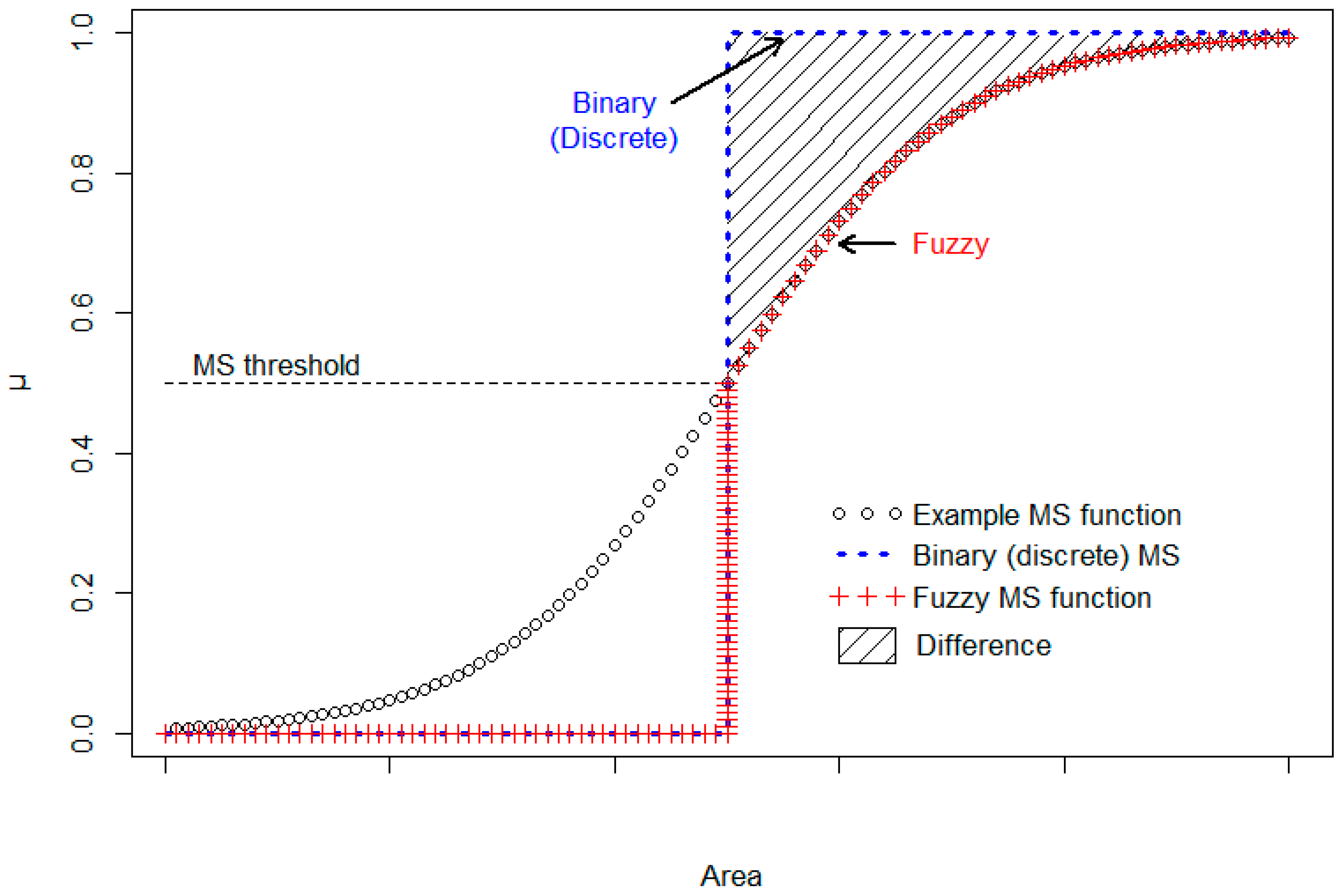
Figure 2) is assigned MS degrees between 0 and 1, expressing how much the data set value satisfies the defined concept (e.g., belonging to riparian zone). An example MSF is depicted in
Figure 3 (black circle symbols). Such MS values belong to a fuzzy set, describing “soft” relations with un-sharp or “fuzzy” boundaries with respect to input factor’s values, in contrast to dichotomic (binary) MS degrees of “hard” classification approaches. MSFs associate MS degrees to the full value range of the input factor data sets.
As a number of factors are used, being grouped to modules, fuzzy sets need to be fused (combined). Finding appropriate connectives for the logical combination of fuzzy sets has turned out to be an important issue [
69]. There are several techniques to combine or group these fuzzy sets, and results can differ significantly depending on the way the data are fused.
The right choice of such a data fusion framework depends on the type and characteristics of data to be managed [
70]. For environmental data of high complexity, often containing imprecise/vague information, a so called hard fusion (
Boolean AND/OR) would not be adequate, since it can easily produce false positives/negatives. Instead, soft aggregation operators such as
AND like/OR like allow a modelling towards AND/OR, and can cope with extreme situations, where e.g., only one/all factor/s is/are satisfied [
71]. In the frame of this study, Generalized Conjunction Disjunction (GCD) aggregation operators [
72,
73] have been applied. GCD allows a soft aggregation (
soft OR/soft AND), which not only can deal with an unlimited number of factors, but also with weights assigned to them. A parameter
r defines the degree of simultaneity or conjunction degree (for
soft AND) and replaceability or disjunction degree (for
soft OR) of the contributing factors, reflecting the required level of satisfaction of these two fundamental logic connectives. The GCD (parameterized in
r) of
m values
vk in [0,1] with importance degrees
ik which sum to 1 is defined as follows:
where
vk are the values to be aggregated,
ik are their relative importance weights,
r is a parameter ranging from −∞ to +∞ and
r ≠ 0 and
Σik = 1. For our purpose we chose a weak simultaneity/replaceability, for which
r values are recommended as
r = 0.26 (
soft AND) and
r = 2.018 (
soft OR) [
73]. A comparable approach has been applied to model rural land abandonment with multi-source data [
74].
2.5. Input Features
Input features are usually generated from original model input data, such as remote sensing data or a DEM. After assigning a MS to the generated data sets, based on an individual MSF (detailed in
Table 3), the data are integrated in the model as depicted in
Figure 2. The characteristics of the applied MSFs, their derivation and MS fusion principles are described in
Table 3 and later in this section.
The path distance (PD) is a frequently used measure to determine the minimum accumulative travel cost of fluids from a source to each location on a raster surface. It was successfully used in previous riparian area mapping [
22]. The PD can be expressed as
with
D as surface distance from source and
Fsl as friction factor determined by the local slope. For longer distances from the source (river) and/or higher slopes, the PD results higher. This general rule is inverted by the applied MSF assigning higher MS degrees to areas closed to the source.
Topography determines largely the gravitational flow of water within the landscape. Local landforms control the hydraulic head, water flow and water distribution [
26]. The topographic wetness index (TWI) [
75] is the most widely used indicator to model the local hydrological behaviour of a varying topography and helps to identify wet or dry sites depending on topography. It is defined as
where
α is the specific catchment area, or drainage area per unit contour width, defined as
A/b; A is the upstream catchment area [m
2], while
b is the contour width [m].
β is the local slope steepness in degrees. The index takes on higher values, if the upstream catchment area increases or if the slope angle flattens, indicating a stronger wetness. Similarly, the adopted MSF assigns high MS degrees to high TWI values.
The “Saga wetness index” (SagaWI) [
76,
77] differs from the classical TWI through the use of a “modified catchment area” (
αm), which aims to alleviate the relatively strong effects of slight terrain variability on the catchment area in zones of typically orohydrologic homogeneous conditions, such as valley floors. This is achieved by iterative modification of each grid cell’s catchment area dependent on neighbouring maximum values, using a slope-dependent equation until the result remains unchanged by additional iterations. As result it predicts for cells situated in valley floors with a small vertical distance to a channel a more realistic, higher potential soil moisture compared to the standard TWI calculation. For these reasons the SagaWI was adopted in this study. The SagaWI has been calculated with the software module Saga wetness index in QGIS Desktop 2.5.1 [
78]
The flood extent zones of the FHM at flood return periods 20, 50, and 100 years were directly assigned a MS degree as outlined in
Table 3.
Soil data: Since an ideal soil parameter such as the soil transmissivity, computed of average saturated hydraulic conductivity and the depth to restrictive layer was not available, an alternative had to be computed. The HWSD provides soil attributes for dominant and associated soils within a soil mapping unit (SMU), providing the share of all composing soils. The following soil attributes were selected: area share of SMU, soil type, available water storage capacity (AWC), obstacle to roots, presence of an impermeable layer, soil water regime, and top soil and subsoil organic carbon content. For all attributes, dedicated MSFs have been associated, while the MS degree for the attribute “share of SMU” is represented by the share itself (
Table 3). All single soil MS were combined by
soft OR aggregation to a single soil MS.
Indicators for vegetation vigour (Normalized Difference Vegetation Index, NDVI) [
38] and leaf water content (Normalized Difference Water Index, NDWI) [
39] provide evidence of riparian features. This is particularly evident in drier areas, where the riparian corridor creates a strong contrast with the remaining land cover. Sigmoid MSFs were applied for both indicators (
Table 3).
Land use/land cover: LCLU classes have been assigned a MS degree according to their probability of being of riparian nature. Typical riparian features, such as “Riparian broadleaved forest” have been assigned a MS of 1, while typical non-riparian features such as built-up areas or agricultural fields have been assigned a MS of 0. MSs of all classes are detailed in
Table S1. LCLU classes which can be of both, riparian and non-riparian nature, have been assigned a so called neutral value, i.e., MS 0.5, in order to keep them in the system. In such cases, the combined final MS is determined mostly by the MS of other input layers.
MS functions were determined by expert knowledge, as in the case of LCLU MSs, or empirically, based on previously mapped riparian zones [
22,
23], by extracting the histogram of the variable of interest and approximating a MSF from it.
For the modelling of riparian zones, it is considered important to take regional differences into account, compensating for soil, geomorphic or climatic particularities. Therefore, a stratification approach was applied through individual adjustments to each of the 43 DUs, applying modifications to the weights (potentially ranging between 0 and 1) of the input layers (i) Path Distance; (ii) SagaWI; (iii) soil data and (iv) the FHM for PRZ delineation. The standard weights for these layers were set to 0.44, 0.17, 0.06 and 0.33, respectively. Adjustments of up to ±0.1 were applied, based on expert judgement by comparing the PRZ extent to high resolution optical satellite data as a reference.
2.6. Model Output
By applying a segmentation together with the above described fuzzy logic based classification approach to the available input features, the following riparian zone delineation products are derived:
- 1
Potential Riparian Zones (PRZ)
- 2
Observable Riparian Zones (ORZ)
- 3
Actual Riparian Zones (ARZ)
A major advantage of the chosen model design is its ability to create these complementary riparian zone delineation products, which represent different aspects of riparian zone occurrence (such as the PRZ and the ARZ), thus enabling further analyses. The ARZ is created as intersecting product of PRZ and ORZ, assuring a higher degree of product reliability, since both data sets are based on independent sources. The ratio ARZ/PRZ provides a first assessment of riparian extent saturation or, if inverted, the riparian extent deficiency, relating the actual riparian extent to the potential one within a defined area. High riparian extent saturation values indicate areas where ARZ is very close to its potential extent, or, in terms of area extent, almost “saturated”. Low values in turn express a low degree of saturation, indicating an extent deficiency. The ratio is deemed a richer indicator as the ARZ and/or PRZ by its own. Assuming that PRZ provides the historic or pristine-like extent of riparian coverage, the inverted ARZ/PRZ ratio provides a dimension for a rough assessment of historic riparian area losses.
In the module PRZ, areas are mapped for their natural disposition to host riparian features, which are not necessarily represented (any more) in today’s actual LCLU class. The disposition is computed for several input layers, which can be added or removed in a modular way. The resulting MSs are combined to a preliminary PRZ, applying a soft OR aggregation (see Equation (1)).
In a last step, standardization is applied to the preliminary PRZ MS raster. That is to ensure that the vector based delineation of the PRZ (MS_PRZ > 0.5) is harmonized with the ones of neighbouring DUs. Based on a threshold (e.g., 0.6) applied to the preliminary PRZ raster, which best fits the PRZ extent at MS μ = 0.5 of neighbouring DUs, a linear rescaling of values lower and higher than this threshold is done, in order to standardize the meaning of the PRZ MS values. The resulting raster is the PRZ MS called MS_PRZ.
In a parallel module, the ORZ is derived, representing the actually observed (often recent) riparian zones, based on different input layers. Again, input layers can be considered modular and are treated and combined the same way as for PRZ. ORZ is based on the observation of certain vegetation classes, as derived from VHR EO imagery through visual interpretation. Additionally, NDVI and NDWI provide further evidence of riparian features. The derivation of the ORZ is done on basis of an object-based processing of the three inputs. Object geometries are created by the application of a segmentation algorithm to the same high resolution multi-spectral imagery as used for NDVI/NDWI calculation (Landsat 8, IRS Liss III; bands red, NIR, SWIR; both resampled to 25 m by bilinear interpolation) and the rasterized LCLU product (cell size: 25 m; mandatory criterion for object differentiation). The segmentation algorithm is the multi-resolution segmentation algorithm as implemented in Trimble eCognition 9.0. The segmentation parameters are: shape = 0.1, compactness = 0.9. The same multi-spectral imagery is used for the calculation of NDVI and NDWI. Each object geometry is associated with
- 1
mean NDVI MS value of the pixels contained in the object geometry,
- 2
mean NDWI MS value of the pixels contained in the object geometry and
- 3
MS value of the LCLU class contained in the object geometry.
The resulting single MSs of all three layers are equally weighted (i = 0.33) and combined (soft OR) to a single MS, expressing the probability to encounter observed riparian features on ground (MS_ORZ). Only exceptions to this rule are those DUs covering (semi-)arid areas, where one or more satellite scenes used as imagery source for the NDWI were acquired during an occurred dry season. In these cases, the NDWI weight within the MS combination process had to be reduced (i = 0.20), in order to maintain a meaningful DU-intercomparability.
MS_PRZ and MS_ORZ are combined via soft aggregation to MS_ARZ (soft AND, with r = 0.26; see Equation (1)), weighting MS_PRZ higher (i = 0.66) than MS_ORZ (i = 0.33).
National or supranational riparian datasets can, if available, be overlaid at this point, leaving the door open for assimilation of such further independent data sources. MS_ARZ (or MS_PRZ) are finalized (i) as vector data sets, by offsetting the MS raster at μ = 0.5; and (ii) left as raster with the according MS values.
3. Results
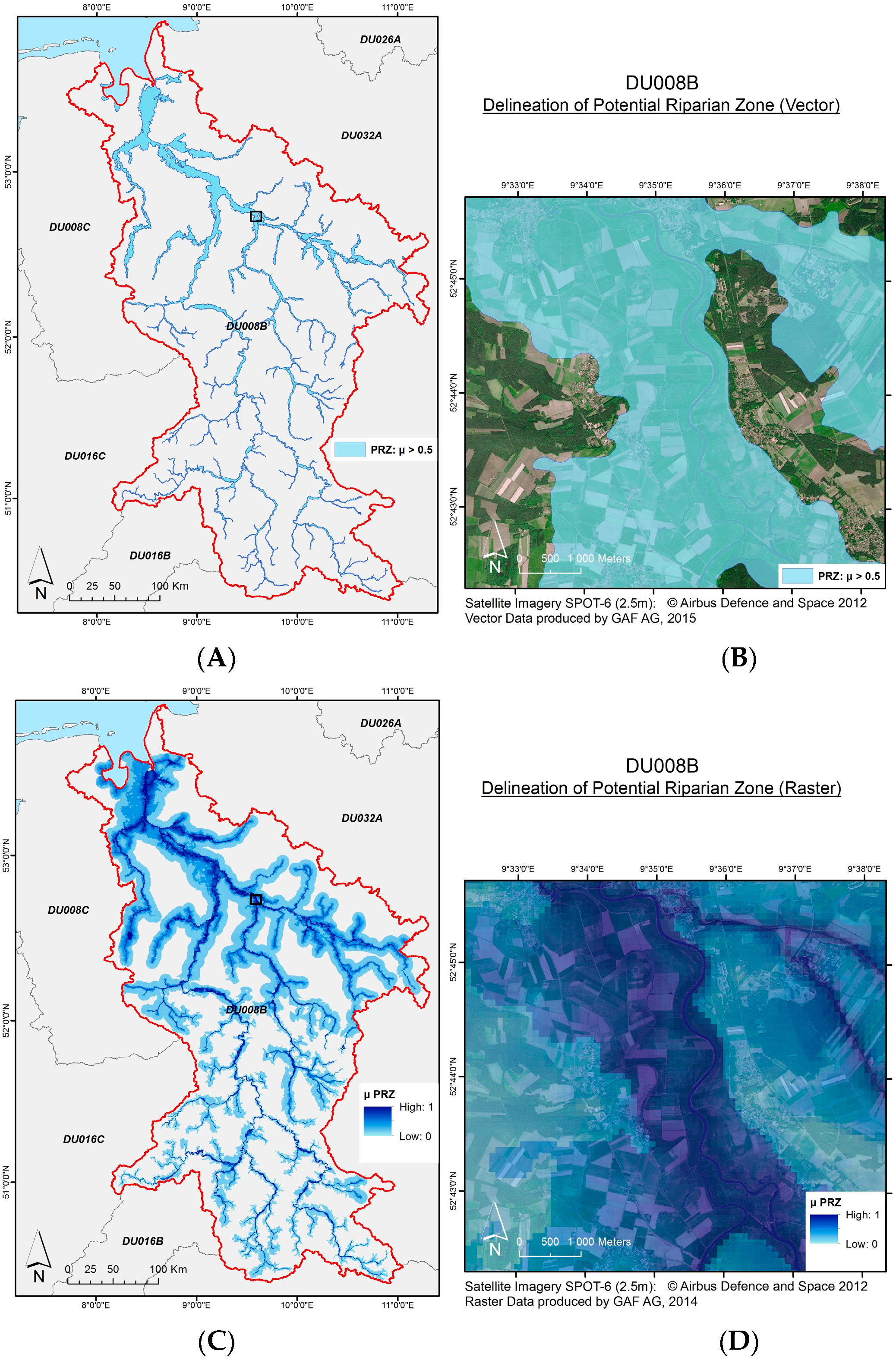
All results are grouped into DUs (see
Figure 1), and can be consulted or downloaded from the Copernicus site [
79]. An example, depicting vector and raster based PRZ results in full resolution for one DU (Weser catchment) is shown in
Figure 4.
To facilitate the (statistical) analysis of the output products on a pan-European extent, they were summarized within 1 km
2 grid cells. Although leading to less detailed data, this processing step avoided or minimized information losses. Besides the high spatial detail, also the fuzzy character of the products required particular attention for statistical analysis. In this regard it is important to keep in mind the concepts of fuzzy and dichotomous (binary) MS (explained earlier) for reading the results. Each of these concepts delivers different results for the areas of ARZ and PRZ. The concepts of fuzziness and dichotomy for area measurements are not applied on the full MS range, but only above
μ = 0.5, as
Figure 3 depicts. Area measurements in binary mode assume a sharp cut-off at the MS threshold of
μ = 0.5, below which no riparian area is being kept or accounted for (accounted as 0), while above it the area is fully considered (accounted as 1, or 100%). Equally not accounted for are riparian areas of
μ < 0.5 when applying the fuzzy area assessment, while above of this threshold, in contrast to the binary approach, area measurements are weighted according to the resulting raster based MS. The difference between binary and the here applied fuzzy area assessment can be quantified by the hatched area in
Figure 3 and depends obviously on the effective shape of the MSF. Full area accounting of pixels above
μ = 0.5, as in the case of binary mode, leads obviously to larger area sums, compared to the fuzzy mode, where the same pixel areas are weighted by their MS.
Application of fuzziness on the full MS range can instead be seen from the detailed mapping example in
Figure 5B,C, where MSs ranging from 0 to 1 are overlaid by a vector based delineation (cut off at
μ = 0.5) for ARZ, ORZ and PRZ. Furthermore, the detailed example shows VHR imagery and the LCLU classification of the area (
Figure 5A,D).
Country-wise and global statistical key numbers of ARZ, PRZ (both fuzzy and binary, named ARZ
fuz/ARZ
bin and PRZ
fuz/PRZ
bin) and other indicators, such as LCLU shares, are reported in
Table 2. Within the study area (EEA-39), a total of 55,558 km
2 have been delineated as ARZ, and 182,488 km
2 as PRZ (fuzzy approach), which represent 0.95% and 3.13% of the total study area (EEA-39), respectively. If accounted in binary way, ARZ amount at 69,128 km
2 and PRZ at 341,215 km
2 or 1.19% and 5.86% of the total study area, respectively. Due to above mentioned reasons, the binary accounting mode delivers hence an ARZ area 24% larger and a PRZ area 87% higher than the respective fuzzy accounting mode.
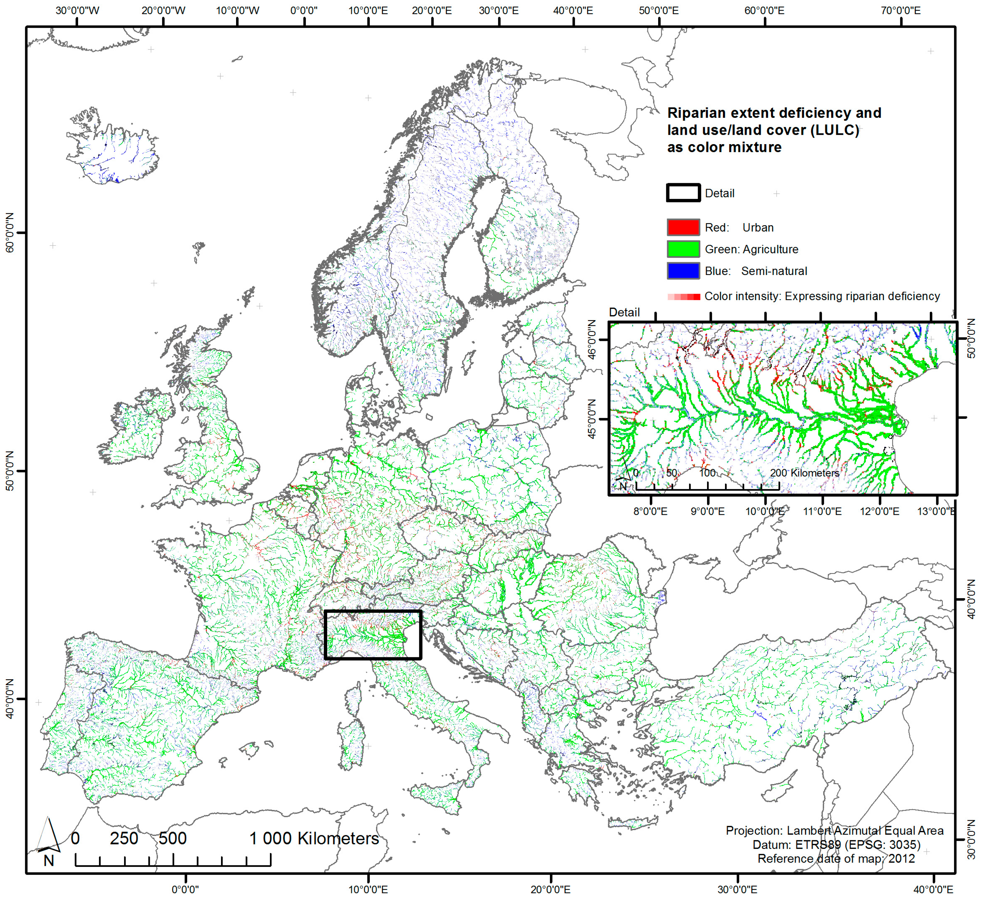
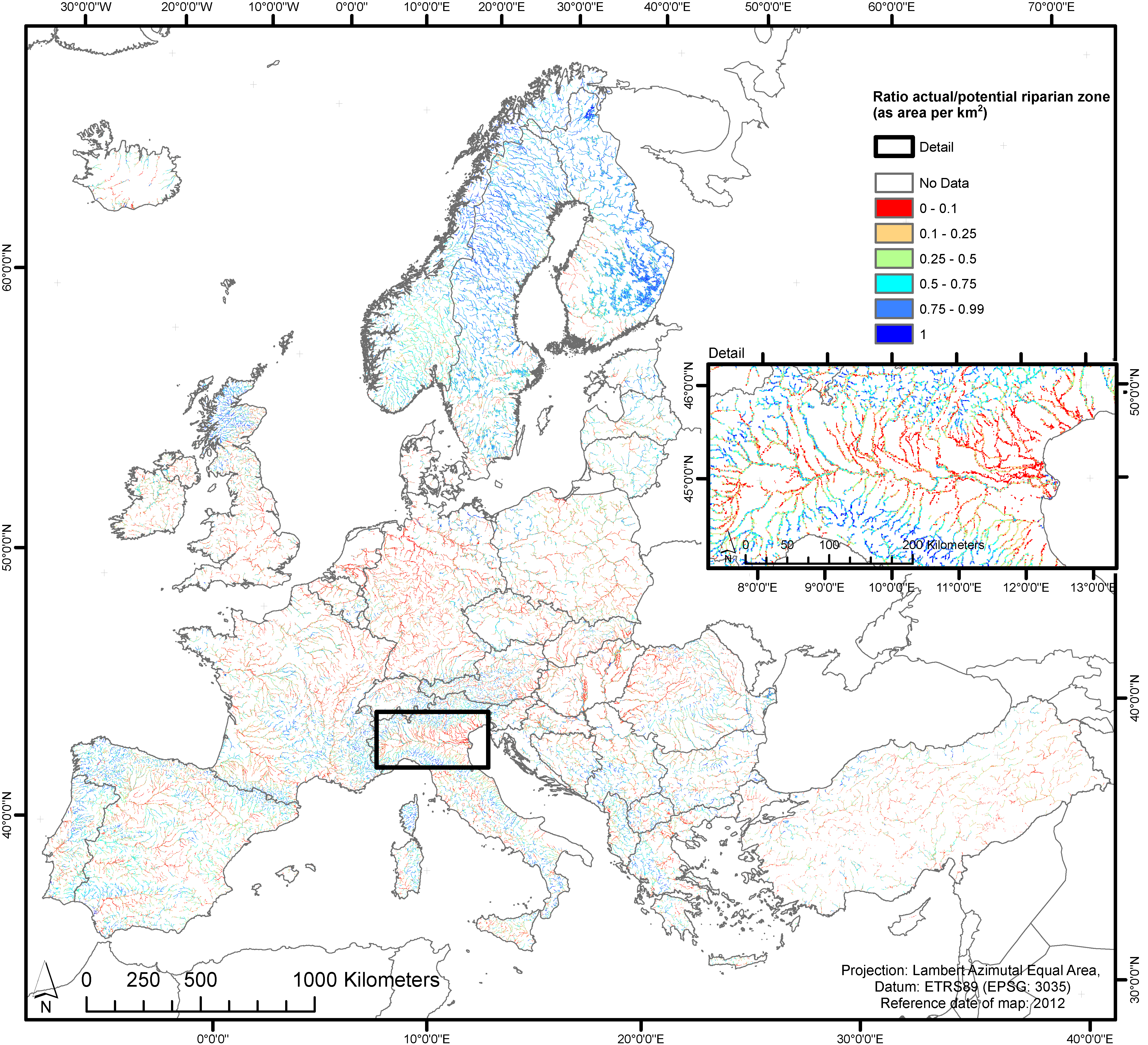
The ratio ARZ/PRZ, calculated on a fuzzy approach, is depicted in
Figure 6. The figure provides quickly an impression of where the riparian areas are close to the full potential, such as in large parts of Scandinavia. For spatially identifying
riparian extent deficiencies (i.e., areas with a low ARZ/PRZ ratio) the situation appears spatially complex. Anyway, some areas such as the Netherlands, large parts of Germany and Eastern European countries, and the Po-valley (shown in detail) can be identified as hot spots of
riparian extent deficiency.
Apart from the ratio values, it is interesting to get an idea about its components, the ARZ and PRZ areas. For EEA-39 country-wise or DU-wise comparison,
Figures S1 and S2 in the section Supplementary data provide graphical overviews of the individual ARZ/PRZ ratio-contributing areas, respectively.
Figure S1 reveals for the three Scandinavian countries Norway, Finland and Sweden (NO, FI, SE) particularly high proportions of ARZ compared to their PRZ areas. The exceptional status of those Scandinavian countries becomes once more evident when examining the overall ARZ/PRZ ratio mean value: the grid cell-wise calculated EEA-39 wide mean (median) amounts to 0.44 (0.40) with and to 0.37 (0.29) without Norway, Finland and Sweden, respectively. The large area contribution (in terms of absolute km
2) of the Scandinavian countries with generally higher ARZ/PRZ ratios increases the EEA-39-wide mean (median) in this pixel-based calculation.
At this point the pressures or reasons for the
riparian extent deficiencies become of interest. In terms of LCLU this can be answered by
Figure 7, where the riparian extent deficiency (as colour intensity) is combined with the three main LCLU categories “Urban” (in red), “Agriculture” (green), and “Semi-Natural” (blue). The green colour, expressing agricultural land use, is clearly dominating this image for most of Europe, whereas in Scandinavia this changes in favour of semi-natural LCLU and locally, especially in highly urbanized areas, towards urban land use. Colour intensity is higher for areas with high riparian extent deficiency.
Table 2 and
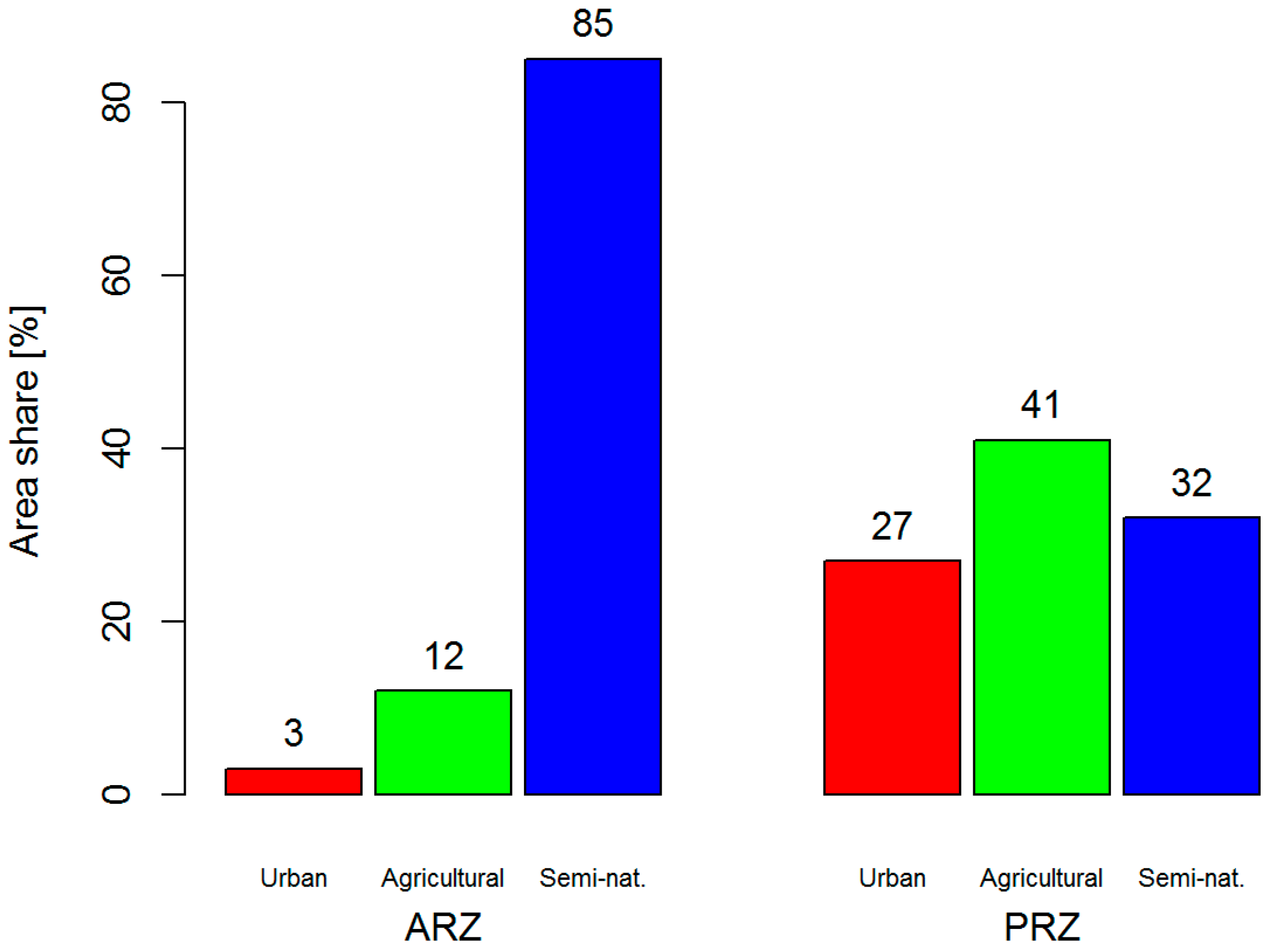
Figure 8 provide more detailed numbers for countries and the full study area in relation to LCLU. ARZ
bin comprise 3% urban, 12% agricultural and 85% semi-natural land. The high area share for semi-natural land is obviously expected, while the urban and agricultural shares can be explained by the presence of green urban areas and in particular agricultural grasslands, respectively.
PRZbin instead comprise 27% urban, 41% agricultural and 32% semi-natural land, indicating that there would be a significant potential for riparian expansion, especially within the land category agriculture. In urban areas, an expansion may be more difficult due to constraints such as built-up areas.
3.1. Sensitivity Analysis
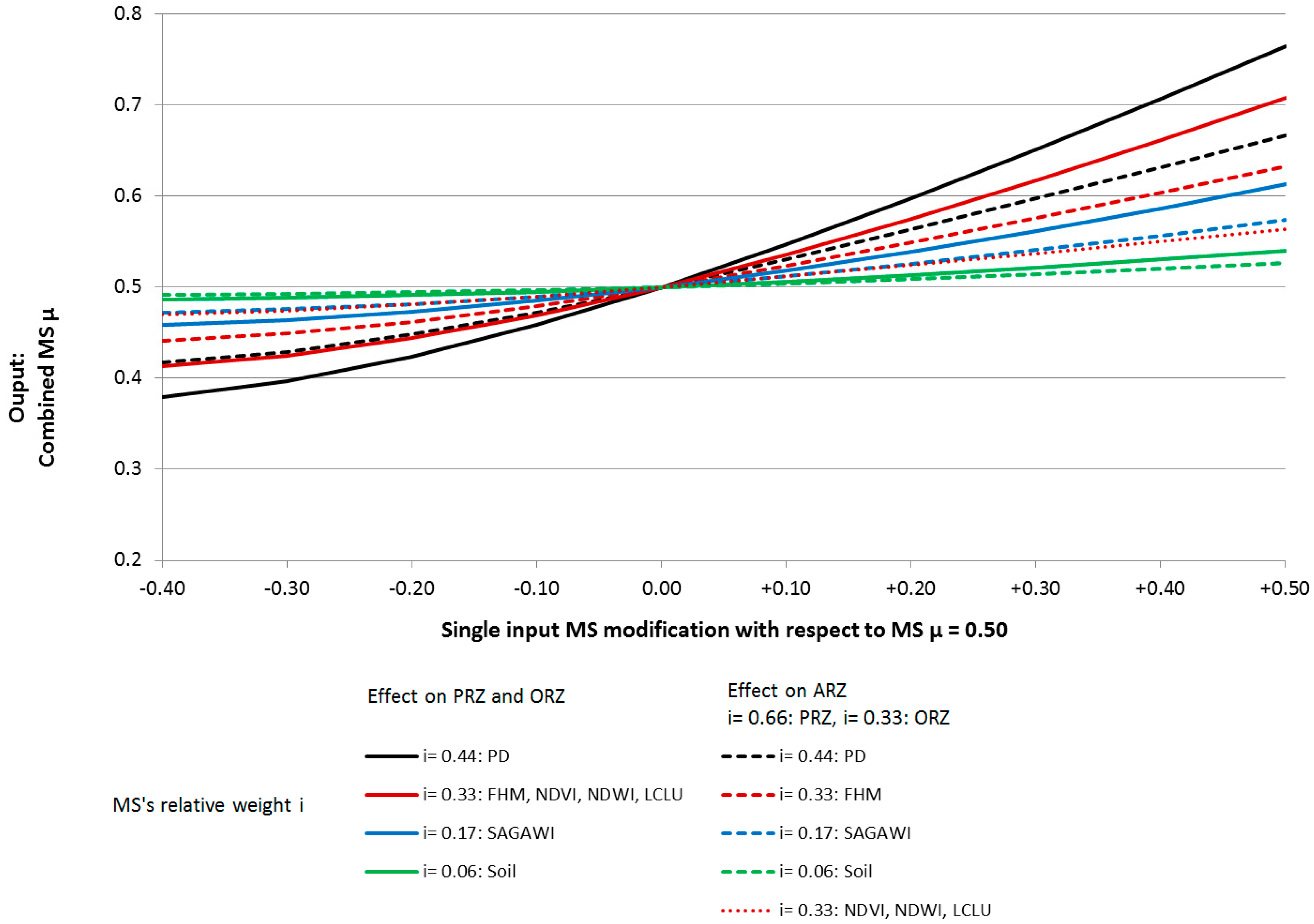
The results PRZ, ORZ and ARZ are sensitive a number of factors. Beyond the availability and the inherent quality of input data sets, the results depend crucially on each input features’ MSF and its applied relative weight
i within MS combinations (see Equation (1)). To understand the effect of varying MS and respective weight
i on PRZ, ORZ and ARZ, a simulation, where a single input feature was varied in terms of MS and weight
i, was set up. MSs of all remaining input features were kept constant at a MS
μ = 0.5. During simulation, the examined MS was increased and lowered by steps of MS = 0.1, starting at a MS degree of 0.5, whereby different weights were applied. The input feature combinations were chosen analogous to the study: first, a SOFT OR combination as applied for PRZ and ORZ, and subsequently, a SOFT AND combination to simulate the fusion of PRZ and ORZ to the final ARZ. Also for the SOFT AND combination one input features MS was set to a constant value of 0.5, while weights were distributed analogous to the study (PRZ:
i = 0.66, ORZ:
i = 0.33). The results are displayed in
Figure 9. The effects of the SOFT OR combination, as it was applied to combine the input features to create PRZ and ORZ, are displayed as continuous lines, at different weight levels, while the effects of the SOFT AND combination, as applied for ARZ, are displayed as dashed lines. Obviously, effects are amplified for higher weights. It can be observed, that generally the impact on PRZ and ORZ is higher than for ARZ, due to the occurring combination of PRZ and ORZ to ARZ. Within this study, the most sensitive input feature is the PD, whose applied weight has been set to
i = 0.44. Its input MS value and hence its inherent data quality, relying on DEMs and river location is of high importance to the PRZ, but this effect is strongly alleviated on the ARZ, as it can be observed. Changes of PD MS degrees of up to ±0.2
μ do not alter the PRZ by more than
μ = 0.1, and the ARZ by not more than
μ = 0.06, while the effects of all other input features are remarkable lower, due to their lower weights.
3.2. Accuracy and Reliability
Due to excessive costs and time constraints, an ad-hoc field validation for accuracy assessment of the riparian zones dataset on the EEA-39 scale was not considered feasible. Alternatively, two strategies were followed to derive indications of the reliability of the ARZ dataset: (i) a qualitative assessment examining and discussing classification errors identified through an extensive visual analysis of the ARZ dataset with Google Earth Pro© observation viewer [
80] and additional VHR imagery; (ii) a quantitative assessment of user and producer accuracy using (a) visual validation points from Google Earth Pro© and (b) independent datasets. Only the ARZ
bin dataset has been validated, due to lack of appropriate validation data comparable to the PRZ.
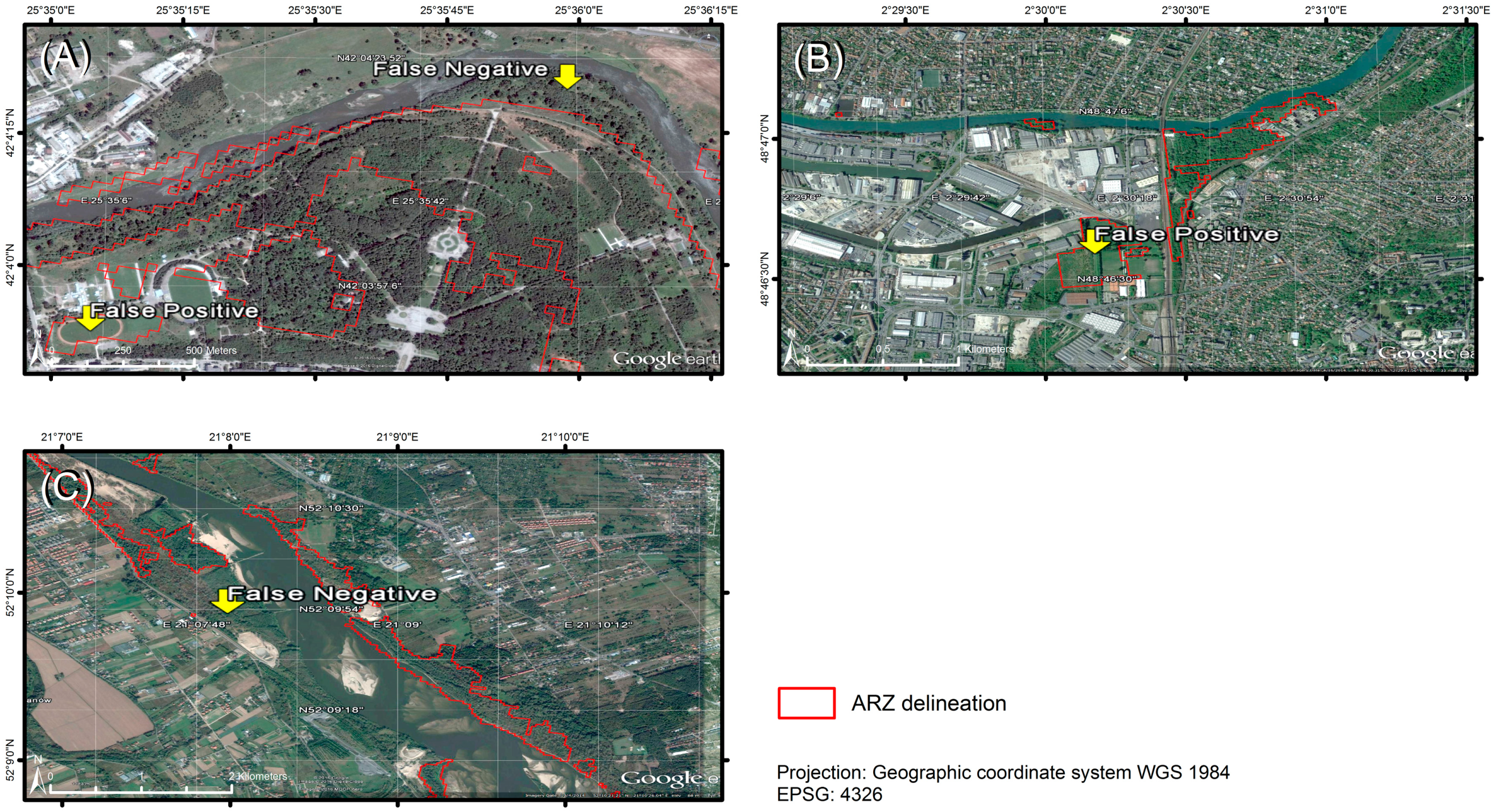
The qualitative reliability evaluation was performed using a set of 11 multispectral VHR images of recent RapidEye, Quickbird and SPOT5 acquisitions, together with Google Earth Pro© imagery. The ARZ were overlaid to the imagery, and three randomly chosen areas (each of approximately 10–100 ha) for each of the 47 DUs were visually analysed, summing up to a total of 141 areas. Overall, ARZ were well represented, appearing to be in general terms a reliable product. Overestimations (false positives) are mostly found: (i) in landscapes with complex agricultural/urban land use/land cover, with classification errors more common in green leisure areas and urban gardens, or in agricultural patches within an urban context; (ii) nearby or within flooded areas; (iii) along tree lines of cemented river channels (
Figure 10A,B). Underestimation errors (false negatives) are mostly identified near or within large floodplains of anastomosed rivers and river deltas, and in some areas where the river network appears underestimated (
Figure 10A,C). Generally, regions with less frequent urban or agricultural land cover reveal higher delineation accuracy.
Quantitative measures of ARZ accuracy were derived on a first instance using visual validation points (VISVAL) from Google Earth Pro© imagery, as applied in previous studies [
22,
81]. Confidence level
δ of classification accuracy estimate
p for large sample sets was calculated following Spiegel [
82]. User’s accuracy (UA) was derived by randomly extracting 200 points (25 × 25 m pixels) from the ARZ dataset, and checking on-screen the number of matches. ARZ UA resulted as 81.5% ± 5.4% at 95% confidence level. Similarly, producer’s accuracy (PA) was calculated by identifying randomly distributed riparian points in Google Earth Pro©, using a 25 x 25 m pixel geometry, and limiting the VISVAL points to the hydrological buffer network used in the ARZ processing. After applying filters for Strahler’s order 3–8 we assessed 225 points and their matches (spatial intersection) with the ARZ dataset. PA resulted as 76.9% ± 5.5%.
As a complementary indication of PA we also exploited three different and independent datasets (i)–(iii) for absence/presence of riparian zones. The datasets are based on: (i) ecological survey of riparian forest (‘alluvial and riparian woodlands and galleries close to main European river channels’), as part of the LUCAS 2009 data [
83]; (ii) River Habitat Survey data (RHS [
84]), a field method for the broad characterization of river streams, from (a) Technical University of Lisbon and (b) various institutions in the context of the MARCE project [
85], coordinated by the University of Cantabria. The dataset was limited to points along streams of Strahler’s order 3–8 and to the hydrological buffer network considered in the ARZ model, resulting in 791 points. To meaningfully represent the extension of each field survey we assigned a 50 m buffer to the riparian point location, and checked spatial intersection with the ARZ dataset. PA resulted in this case as 80.0% ± 2.79%. Overall, the quantitative accuracy assessment was performed with a total of 1216 sampling points (matches = 969), leading to an overall accuracy of 79.7%.
Figure S3 shows the spatial distribution of all validation points with distinct symbols for each type of validation and validation outcome. Based on these points, no spatial patterns of match/mismatch were observed, although it should be noted that North Spain and Portugal have been sampled more frequently by the independent datasets used for the UA assessment. Matching and mismatching sampling points were tested for dependencies with respect to Strahler’s order and to the size of ARZ polygons they fall inside (
Figure S3). The results display a regular pattern for stream order dependent accuracy and apart from generally larger ARZ areas for the UA assessment, no particular occurrences.
4. Discussion
The results achieved within this work are of high importance to a wide range of disciplines, among them policy makers and land or water (restoration) planners, researchers, engineers, water-basin managers, ecologists and economists. The pan-European extent and the consistent method of data derivation facilitate actions on a large scale, such as of EU-policy making. With respect to existing data sets, the gap for a uniformly derived dataset covering the whole EEA-39 area whilst being of high spatial detail is filled. A multitude of input data, including topographic, hydrological, soil and EO-based data is employed. The yielded results are not comparable to the previously derived JRC riparian zones but represent a data set of higher value, providing more detail, accuracy and reliability, considering the approaches applied and the input data sets employed. For example, the hydrological network, based on EU-Hydro, in combination with the VHR LCLU dataset of riparian zones, has been derived based on optical remote sensing data, from which the geo-location of rivers was precisely captured, in contrast to the hydrological network of the JRC data set, where river locations are mainly based on a drainage network based on the SRTM-DEM. Another example is the LCLU MMU, which has significantly improved from CORINE’s 25 ha to 0.5 ha. Accuracy improvements have been achieved also for the applied EU-DEM, which in Nordic countries was substituted by more reliable national data sets. Apart from data input quality improvements, the multitude of input data sets is expected to significantly increase the reliability, since, similar to a weight-of-evidence approach, a repeated affirmation of an attribute leads to more robust results. A crucial improvement of the riparian zones delineation model compared to previous works is its completeness, covering not only semi-natural areas, but all kind of land cover/land use categories. Moreover, the applied concept with multiple outputs ARZ, ORZ and PRZ enables a much wider use of results. A number of novel applications should become possible, e.g., in ecological fields such as ecosystem service and function analyses, through the additional availability of the PRZ, the ORZ, the ratio ARZ/PRZ and the LCLU data set derived in parallel.
The implementation of this work required an effort from policy side, managing present and future ecological needs, such as ecosystem services and biodiversity monitoring. It also required significant investment from a technical-scientific body carrying out a vast and complex work. The present article describes indeed not one but several output data sets within the riparian context, i.e., mainly the ARZ and the PRZ. Synergistically, a detailed VHR LCLU dataset is available in parallel, covering the wider riverine zone of all rivers of Strahler’s stream order ≥3. Each data set and specifically their combination, provide an excellent starting point for more detailed analyses in the riverine and riparian domain. Data downloads are organized in Delivery Units (DU), which are based on an aggregation of ECRINS river (sub-)catchments. This way, a separate and independent processing of each DU can be performed without running into technical issues of data processing.
Methodologically, the riparian area delineation approach can be divided into two work tasks: the derivation of (i) ARZ and (ii) PRZ (and intermediate result ORZ), while the LCLU classification is considered a parallel task, which in other cases might not be required to be computed. Only the foreseen independency of the modules ARZ and PRZ enables finally the contextual interpretation of their resulting end-products, i.e., by means of the ARZ/PRZ ratio. PRZ is based on the hydrological data set (river network), terrain topography (slope, height above water level), soil properties, flood zone delineation and LCLU class water. Following a fuzzy MS approach, MSs are assigned to each contributing layer, following defined MS functions. In GIS-terms, an OBIA approach has been applied, where the atomic unit is an object, defined as a polygon with relatively homogeneous conditions, created by a segmentation process. The segmentation and the fuzzy MS approach was applied analogously to the ORZ, where the input data sets are constituted by LCLU data and the EO-data derived vegetation indices NDVI and NDWI. ORZ and PRZ are combined to the ARZ. The multitude of input data sets requires strong efforts in terms of processing and labour, but contributes to higher robustness and accuracy reducing the effect of single bad data values. The model design keeps the door open for further input datasets, potentially becoming available in the future (e.g., by expanding the model to all Strahler’s stream orders).
The accuracy analysis of ARZ
bin was performed by different approaches, amongst others employing independent data sets. The quantitative assessment revealed similar accuracies for both UA and PA, and for visual analysis and independent sources, ranging in all cases around 80%, which can be considered in line with good mapping practices [
86]. The achieved accuracy is deemed a good result, considering the continental-scale extent of the study area and the complexity of the task.
In terms of model sensitivity, the applied data combination method to create meaningful products plays, apart from data availability and inherent quality, an important role. For example, the European FHM was not available for Turkey, which could potentially lead to less reliable results in this area. With respect to the sensitivity of data combination on the results, the assigned MS to the PD has been identified as input feature of highest importance. This is due to its relative high weight within the combination process to derive PRZ. The effects on the PRZ are considered acceptable and the effects on ARZ are even less pronounced. A simulated data combination demonstrated that the result’s sensitivity is not only critically dependent on the applied weight of the input feature within the combination process, but also that PRZ and ORZ is clearly more sensitive than ARZ. This is due to the alleviating effect of the final soft AND combination, where PRZ and ARZ are combined to the ARZ.
A basic analysis on European/national and DU-scale provides statistical figures and plots of the features considered most important. A key indicator is considered the ratio ARZ/PRZ, providing the relation of actual and potential riparian zones and this way the degree of riparian extent saturation, or, if inverted, the degree of riparian extent deficiency. The combination of the ratio ARZ/PRZ and the LCLU data allows an assessment of the drivers of long-term or historic riparian area loss, which was discovered to be predominantly conversion to agricultural use.
However, it is crucial to note that statistics depend significantly on the riparian area inventory approach applied. Here, two different approaches, a fuzzy and a binary one, have been adopted. If considering the whole study area (EEA-39), the binary approach delivers an ARZ area approximately 24% higher than the area based on the fuzzy approach. For PRZ, the binary based figures are by about 87% higher compared to the fuzzy approach. The higher discrepancy between PRZ accounting modes indicates that PRZfuz exhibits generally lower MS degrees compared to ARZfuz. This is expected, since the uncertainty of ARZ, due to a higher number of input layers (sum of ORZ and PRZ input layers) compared to PRZ, is reduced. Also, the PRZ intrinsic uncertainty can be expected to be higher, linked to higher difficulties to determine its area compared to ARZ.
If looking at the shares of ARZbin in between urban, agricultural and semi-natural areas, only a small part of ARZbin is found in urban (3%) and in agricultural areas (12%). The majority is dominated by semi-natural areas (85%). PRZbin instead, is predominantly covered by agriculture (41%), followed by semi-natural areas (32%) and urban areas (27%). These numbers leave space for policy action (e.g., conversion, co-existence, protection), in particular the revealed high share of agricultural land. Urban areas might be more difficult to handle, since they are constrained by built-up areas.
The country-wise and DU-wise relation of ARZ/PRZ ratios dependent on the individual ARZ and PRZ absolute extents has been quantified and visualized by
Figures S1 and S2, respectively. Scandinavian areas (NO, SE, FI) exhibit a particularly high abundance of ARZ. This becomes even more evident when looking at the global pixel based mean and median for the ARZ/PRZ ratio, which amount at 0.44 and 0.40 with and at 0.37 and 0.29 without Norway, Sweden and Finland. Here, due to their large extent, the Scandinavian areas tend to raise these values. However, the pattern of the ARZ/PRZ ratio is not just higher in Nordic areas, but is highly variable also across micro-regions. The clear meaning of this ratio and its ease of calculation makes this indicator a valuable tool for planning.
The potential use of the data set is wide-spread: on top of all applications stands certainly an analysis which goes beyond the one presented in this paper, which helps to understand the roots of a variety of underlying drivers, helps geo-locating them, and provides basis for river restoration. For land/water planners the data could provide important insights for large scale river restoration and filter (buffer) design, as for example with respect to placement or design of riparian filter strips, or how to alleviate nutrient/pesticide emissions to waters. Policy makers may understand better how to allocate funds for effective counter-measures to pollution and plan future actions. Flood mitigation planners may extract useful information to plan (bio-engineered) flood retention basins. Ecologists or related professions may analyse the status of riparian areas, their longitudinal/lateral connectivity and fragmentation, their quality e.g., regarding biodiversity and find the hotspots for interventions. A number of other applications not listed here do obviously exist. For most applications, the pan-European extent provides a tool for action targeting, or in other words, in which places/regions to invest first, in order to reduce the highest risks or to maximise revenue. Obviously, for detailed scale planning more accurate data sets will need to be considered.
A limitation of the data set is certainly the exclusion of the headwaters or rivers of Strahler’s stream order 1–2, being justified by cost considerations. The missing headwaters can be of particular relevance when assessing ecosystem services such as filter or retention capacity, generally known to be higher in lower stream orders, due to preferential non-concentrated flow in these areas. However, this part can be integrated in a second step.
Other limitations concern the variety and quality of input layers. While the quality of the Digital Elevation Model and the hydrological network has been improved compared to the version used for the JRC riparian map, other data sets lack still detail and consequently accuracy, such as the soil maps. The effect of such a rough scale (1:1M), although gridded into 1 km2 pixels, was alleviated with a lower weight (<0.2) for soil data when combining the data within the processing chain.
Finally, it has be acknowledged, that a data set of continental extent is unavoidably subject to simplifications and cannot provide the level of detail and accuracy that a field based local data set would do. Minor riparian areas might be missing or not interpreted correctly, leading to omission or commission errors. The large study area required the employment of a high number of satellite images, of which the majority but not all refer to the reference year 2012, in certain areas potentially leading to a broader time window of interest.
It should be stated very clearly that this work is focused on the riparian area extent and not on its ecological quality, i.e., issues related for example to recent shifts from native to alien plant species are not assessed within this work.


 ,
, 


