Long-Range WindScanner System

Abstract

The technical aspects of a multi-Doppler LiDAR instrument, the long-range WindScanner system, are presented accompanied by an overview of the results from several field campaigns. The long-range WindScanner system consists of three spatially-separated, scanning coherent Doppler LiDARs and a remote master computer that coordinates them. The LiDARs were carefully engineered to perform user-defined and time-controlled scanning trajectories. Their wireless coordination via the master computer allows achieving and maintaining the LiDARs’ synchronization within ten milliseconds. The long-range WindScanner system measures the wind field by emitting and directing three laser beams to intersect, and then scanning the beam intersection over a region of interest. The long-range WindScanner system was developed to tackle the need for high-quality observations of wind fields on scales of modern wind turbine and wind farms. It has been in operation since 2013.

1. Introduction

Measurements of the wind velocity in the Atmospheric Boundary Layer (ABL) provide the means for improving our understanding of a diverse range of flow phenomena and wind conditions, which play an important role in wind energy. In the past, wind measurements were typically acquired using the well-established in situ techniques with sensors, such as cup anemometers [1], mounted on a meteorological mast at heights usually occupied by the lower half of the wind turbine rotor swept area [2,3]. The number of meteorological masts employed to collect the information on the wind flow greatly depends on the application of the wind measurements. The measurements from at least one meteorological mast are necessary for wind turbine power curve estimation [2], while for field campaigns focused on improvement of wind energy flow models, the number of meteorological masts can be up to ten or more [4,5].

However, since today’s modern large wind turbines operate between 60 and 300 m above the ground level, the application of the in situ techniques is becoming extremely expensive due to the costs of tall meteorological masts.

An alternative technology emerged around the turn of the century. Due to the increased availability of fiber-optic components, it became economically and practically feasible to build Coherent Doppler LiDARs (CDL) suitable for operational measurements in wind energy [6,7,8,9]. Before this, CDLs were based on expensive open-space optics, which are voluminous and hard to maintain in field operation. As a result, CDLs were essentially unused in the wind energy community.

Unlike the mast-mounted sensors, CDLs acquire wind observations remotely, without contact with the moving air. They do this by emitting the laser light and coherently detecting the Doppler shift in the backscattered light. The Doppler shift, the frequency difference between the emitted and backscattered light, is a direct measure of the radial or Line Of Sight (LOS) velocity, which is equal to the wind velocity projected on the laser light propagation path.

As mentioned, CDLs are only able to measure radial velocity. However, by using single-Doppler retrieval techniques, such as Velocity Azimuth Display (VAD, [10]), Doppler Beam Swinging (DBS, [11]) or integrating Velocity Azimuth Process (iVAP, [12]), and assuming horizontal homogeneity of the flow, single CDLs are able to provide single-Doppler retrievals of two horizontal or all three components of the wind vector.

Highly accurate single-Doppler retrievals of wind speed have been reported in flat terrain and offshore [13,14], where the flow is expected to exhibit a high degree of horizontal homogeneity. In complex terrain, where the flow is less horizontally homogeneous, CDL estimation errors of up to 8% have been reported [15]. Errors this large are unacceptable for wind energy applications. As a guide, in flat terrain, the best cup anemometers (Class 1a) have an uncertainty (k = 2) of at least 1% at 10 m/s. Including calibration and mounting uncertainty, the total uncertainty is usually between 2% and 3%. In complex terrain, the cup uncertainty is likely to be significantly larger.

As indicated in [16], there are two solutions to this problem, either to correct the data using flow models [15,17,18] or to develop new CDL instruments that do not demand the horizontal homogeneity of the flow to produce accurate retrievals. The correction methods can potentially reduce errors [16]. CDL data correction methods are more successful on sites with a simple to moderate complexity [15,19], than on sites with high complexity [15]. Furthermore, the corrected data accuracy is heavily dependent on the flow model choice and the model’s parametrization [18]. As described in [18], besides the LiDAR data correction methodologies developed by research groups, also companies, such as Meteodyn WT, WindSim and Leosphere, introduced commercial LiDAR data correction algorithms. Specifically, Leosphere developed a real-time correction algorithm, known as the Flow Complexity Recognition (FCR), which is available as an add-on to their LiDAR software [20].

Overall, an improper choice of the flow model and an incorrect model parametrization can potentially introduce additional errors to single-Doppler retrievals. This leads to an increased uncertainty in the single-Doppler retrievals. Furthermore, as the single-Doppler retrievals undergo modifications based on flow modeling results, they do not represent direct measurements of the wind vector.

CDL errors in complex terrain originate from using one instrument scanning in several different directions assuming the flow to be homogenous when this is not the case since the different beam directions (originating from the same point) will sense the flow in physically different locations. In order to have beams sensing in the same location, it is necessary to have the origin of the beams separated. This can be achieved with a multi-Doppler LiDAR, which eliminates the requirement for the horizontal homogeneity of the flow and provides direct wind vector measurements (multi-Doppler retrievals). At least two independent radial velocity measurements are required to measure two components of the wind vector if the other component is known (e.g., assumed to be zero or small compared to the other two components), while to fully characterize the three-dimensional wind vector, a minimum of three independent radial velocity measurements is necessary at any given time. This is possible with three spatially-separated LiDARs.

Since the 1980s, dual-Doppler LiDAR setups were used in several prominent atmospheric experiments. In the Joint Airport Weather Studies (JAWS), two scanning CDLs were used to study convectively-driven downdrafts and resulting outflows near the surface [21]. For the purpose of the investigation of the boundary layer transport and dispersion processes in the urban canopy, a dual-Doppler LiDAR was employed to provide measurements of the urban canopy flows during the Joint Urban 2003 experiment [22,23,24,25]. Within the Invest-to-Save Budget Project 52 (ISB52) simultaneous measurements from two scanning CDLs were used to retrieve dispersion relevant parameters [26]. The instrumentation setup of the Terrain-Induced Rotor Experiment (T-REX) included two scanning CDLs [27] operating simultaneously providing observations of rotary flows in complex terrain [28].

In wind energy-related studies, dual- and triple-Doppler LiDAR setups were not used until recently. During the Musketeer experiment, three CDLs were configured to steer and intersect their laser beams above a sonic anemometer mounted at a mast 78 m above ground level [29]. This experiment demonstrated the feasibility to accurately measure all three components of the wind vector using a triple-Doppler LiDAR. Virtual tower measurements using three scanning CDLs were demonstrated in [30]. In the study [31] two scanning CDLs were used to resolve two components of a single-turbine wake in a vertical plane, while the authors in [32] explored the possibility of acquiring a turbine-scale wind field measurements using a dual-Doppler LiDAR.

In the aforementioned dual- and triple-Doppler setups, the CDLs functioned independently from each other; thus, there was no central computer that would provide and maintain the CDLs’ synchronization. In [32], the authors explicitly stated that after a certain period of time, two scanning CDLs started to drift apart, while the authors in [25] commented that achieving the synchronization among scanning CDLs in field operation represents a challenge. From the operational point of view, monitoring several independent CDLs during the field operation is laborious and often complex since the LiDAR operator has to take care of each of them separately. In all studies, CDLs performed simple scanning strategies typically consisting of Plan Position Indicator (PPI), Range Height Indicator (RHI) and/or step-stare scans. As the CDLs used in the aforementioned studies were typically commercial products, it is well known that their configurability is limited. It does not provide accurate timing of scans required for achieving the strict synchronization among several CDLs, nor sufficient freedom to design more complex scanning methods.

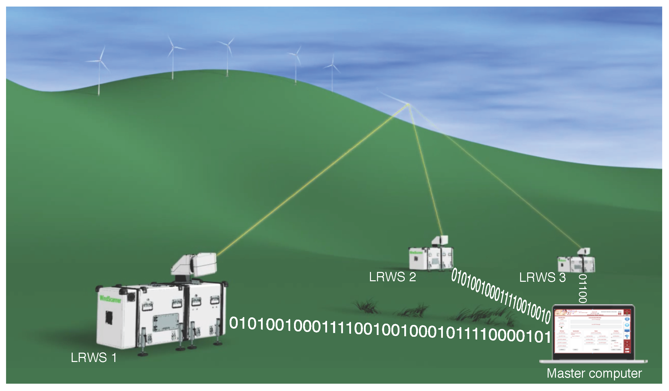
In the WindScanner.dk project [33] we addressed the topics of multi-Doppler LiDAR synchronization, higher configurability and simpler operation. During this project, we were determined to develop highly configurable triple-Doppler LiDAR instruments, know as WindScanner systems, consisting of spatially-separated and synchronized scanning CDLs managed from a central computer unit, known as the master computer. The result of the WindScanner.dk project are two multi-LiDAR instruments known as the short-range and long-range WindScanner systems [34]. The WindScanner systems are intended for detailed measurements of wind fields. The short-range WindScanner system is intended for high-frequency observations of fine flow structures around a single turbine rotor, whereas the long-range WindScanner system is intended for measurements of wind fields on scales of a single and multiple wind turbines. These two systems are complementary to each other. This paper is focused on the long-range WindScanner system.

The paper is organized as follows. Section 2 introduces the design requirements for the long-range WindScanner system. Hardware components, operational principles and software capabilities of the single CDL of the long-range WindScanner system are given in Section 3. Section 4 describes the approach in forming the long-range WindScanner system. How CDLs are synchronized using the master computer is explained in Section 5. Section 6 consists of an overview of field campaigns performed with the long-range WindScanner system. Finally, Section 7 discusses results and future work, while Section 8 gives our concluding remarks.

2. Design Requirements

In order to formulate the design requirements for the long-range WindScanner system, both in terms of hardware and software, we start this section by defining the performance requirements.

First, the idea was to develop a system of multiple CDLs that is able to provide synchronized measurements of all three components of the wind field at points defined by the user. The synchronization allows for turbulence statistics analysis and shorter time averages of measurements. Second, the points are to be distributed in the large volume of the ABL, where the dimensions of this volume should correspond to the dimensions of modern wind farms. This approach allows thorough investigations of the flow field surrounding wind farms. Third, the measurements are to be processed in real-time to provide the possibility of using them in the real-time control of wind farms. Fourth, the system should be configurable such that it can provide substantial freedom in designing measurement campaigns. Finally, we envisaged a diverse range of the system deployments (e.g., offshore, complex terrain, etc.).

Based on these preferences, the design requirements were as follows:

• The system will consist of at least three spatially-separated CDLs
• Both the motion control and CDL measurement acquisition will be performed locally on each individual LiDAR
• CDLs will be coordinated from a remote computer
• The coordination will be achievable using mobile networks
• CDLs are to be pulsed in order to achieve long-range measurements
• The backscattered signal will be processed in real-time yielding real-time measurements of the radial velocity
• The accuracy of the retrieved radial velocity will be at least 0.1 m/s
• The acquisition rate of consecutive LOS measurements can be different
• Several hundreds of configurable range gates will be available for the user
• Range gates will be freely positioned along each LOS
• Each CDL will contain a fully-steerable scanner head
• The pointing accuracy of each CDL will be better than 0.1${}^{\circ }$
• Scanning strategies will include user-defined scanning trajectories
• Scanning trajectories will be time controlled

3. Engineering a Single Scanning CDL

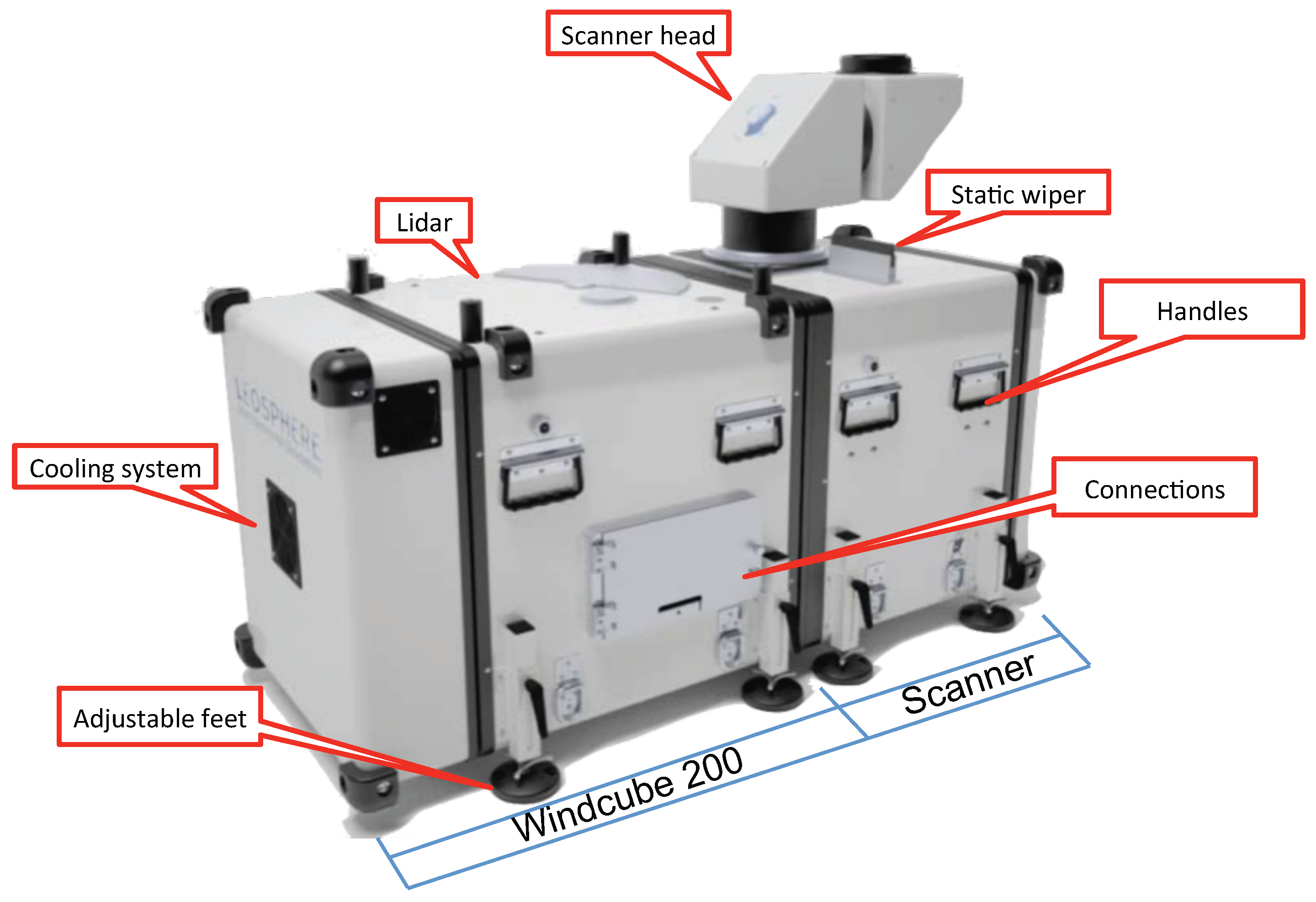
DTU Wind Energy and Leosphere engaged jointly in developing a scanning CDL Long-Range WindScanner (LRWS) based on the pulsed CDL Windcube 200 and a dual-axis mirror-based steerable scanner head (Figure 1,

Table 1. Operational parameters.

Size	1.5 × 0.55 × 0.65 m
Total weight	180 kg
Peak power consumption	1.7 kW
Ingress protection code	65
Temperature range	−10 to 40 ${}^{\circ }$C
Eye safety	IEC 60825-1

). Windcube 200 is based on the technology that has been developed by the Office National d’Etudes et de Recherches Aérospatiales (ONERA) and transferred to Leosphere for commercialization [35,36]. This all-fiber LiDAR consists of commercially available telecom components at 1543 nm and a high power fiber laser amplifier. The scanner head, developed by DTU Wind Energy with expert support from specialized industrial partners, was added to Windcube 200 to provide full dome user-defined steering of the laser beam to the atmosphere. The LRWS is designed to allow assembly of the entire CDL using two standard Windcube 200 enclosures and, thus, the integration of both LiDAR and scanner into a twin compact casing. This approach allows for the separation of mechanical and optical components during transportation, and it simplifies maintenance.

3.1. Transmitter

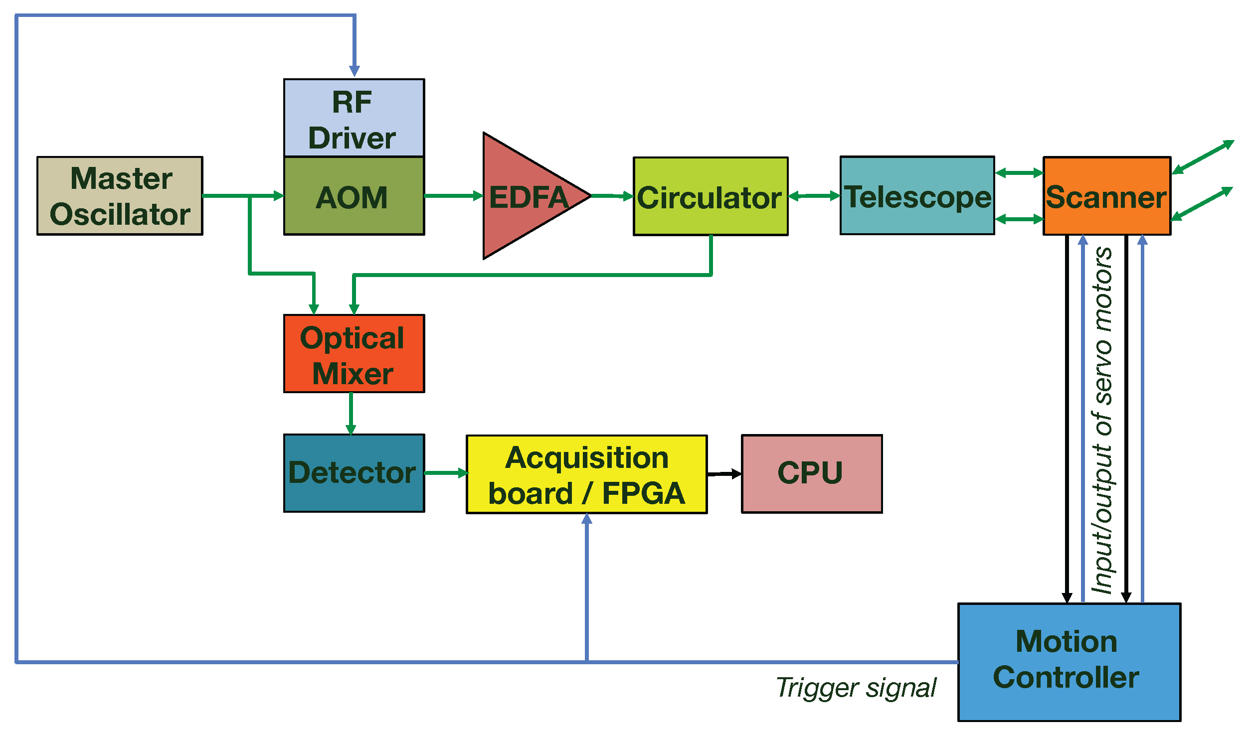
We are using a Master Oscillator Power Amplifier (MOPA) configuration for the transmitter (Figure 2). A Distributed Feedback (DFB) diode laser is used as the master oscillator. The DFB emits a Continuous Wave (CW), frequency stable, polarized, low power, single-mode laser beam.

An Acousto-Optic Modulator (AOM), driven by a pulsed radio-frequency signal from a Radio Frequency (RF) drive, transforms the incoming CW laser light to the laser pulse train. Each emitted low power pulse has a predefined waveform (near Gaussian shape) and frequency offset of 70 MHz. Low power laser pulses are then amplified in an Erbium-Doped Fiber Amplifier (EDFA) and emitted with a Pulse-Repetition Frequency (PRF) between 10 and 40 kHz. The frequency offset enables the detection of positive and negative Doppler shifts, and the high PRF makes it possible to maintain good range performance using a lower pulse energy [37].

We are using three configurations of the pulse waveform, energy content and corresponding PRFs (

Table 2. LRWS characteristics.

Wavelength	1543 nm
PRF	10, 20 and 40 kHz
Pulse length	400, 200 and 100 ns
Probe length (FWHM)	70, 35 and 25 m
Energy per pulse	100, 50 and 25 $\mathsf{\mu }$J
Mean power	1 W
Accumulation time	10 to 10,000 ms
Velocity range	−30 to +30 m/s
Range	50 to 8000 m

), which provide optimization of the measurement process with respect to the desired range and probe length. The probe length in Table 2 represents the Full-Width Half Maximum (FWHM) of the total probe length.

Following the EDFA, the laser beam consisting of the pulse train is magnified, collimated and focused typically at around 1.2 km using a 100-mm aperture telescope. These processes optimize the laser power distribution along the laser light propagation path and decrease divergence in the far field, resulting in an improved Signal-to-Noise Ratio (SNR) at a long range.

3.2. Scanner

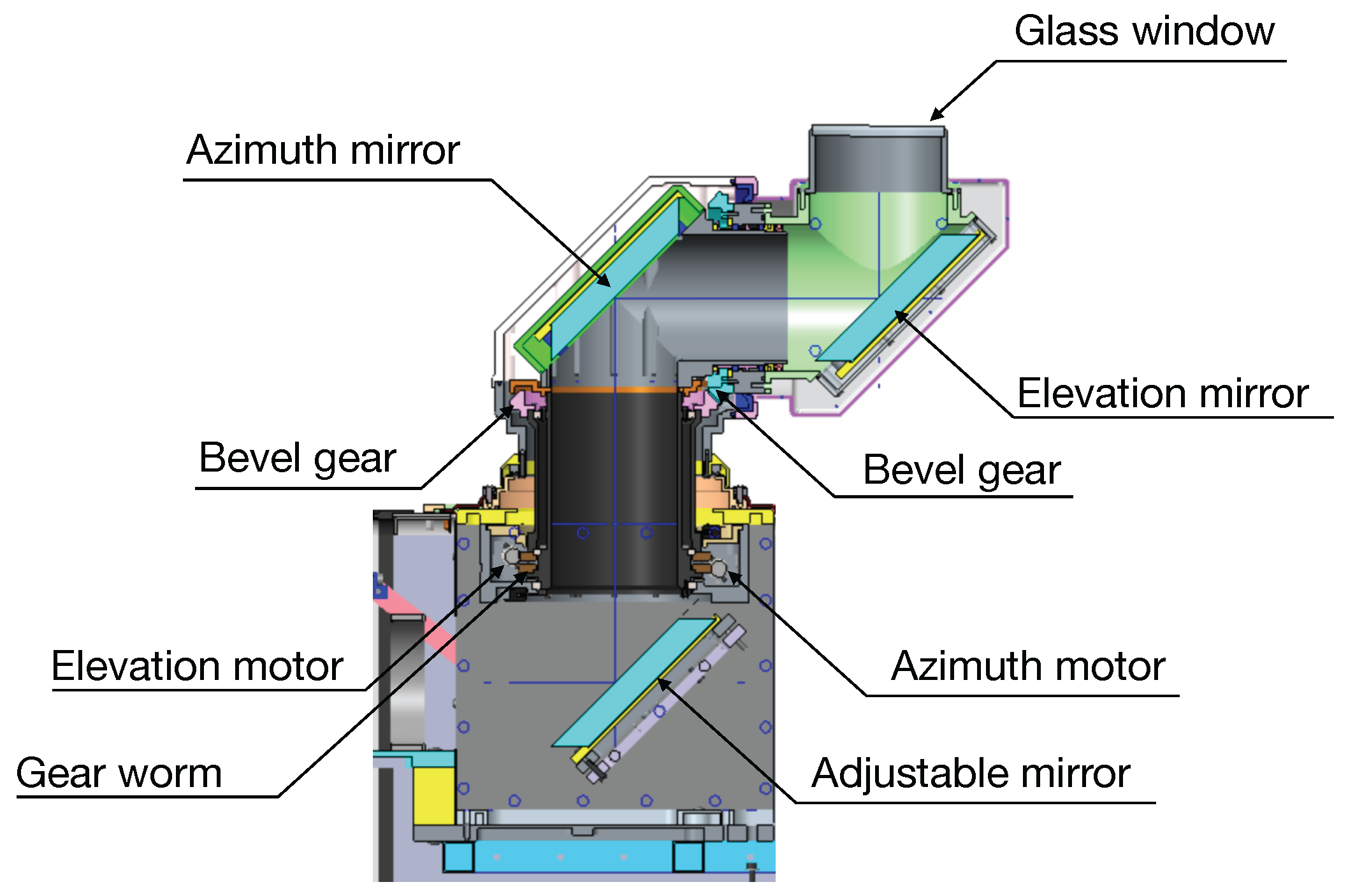
The steering of the laser beam towards the points of interest is performed by means of one fixed and two rotating flat and elliptical mirrors installed in the gear box-driven scanner head with two degrees of rotational freedom (

Table 3. Scanner characteristics.

Moving load	25 kg
Maximum speed	50 ${}^{\circ }$/s
Maximum acceleration	100 ${}^{\circ }$/s${}^2$
Rotation mechanism	Gear-box
Rotation	Endless and continuous
Backlash	<0.03${}^{\circ }$
Azimuth coverage	0 to 360${}^{\circ }$
Elevation coverage	−180 to 180${}^{\circ }$
Clear aperture	120 mm

, Figure 3). Each mirror is fixed to the corresponding mount using a silicon-based glue.

The mount of the adjustable mirror is installed on the non-movable part of the scanner head located next to the telescope exit, whereas the remaining two mirrors, known as the azimuth and elevation mirrors, are connected to the rotating parts of the scanner head. The rotation of the mirrors is achieved using a set of gears and two brushless DC servo motors enclosed in the compact drive unit of the scanner head.

The azimuth mirror mount is directly connected to the azimuth worm gear, which is driven by the worm attached via a flexible coupling to the motor shaft. In order to attain a minimum level of backlash, the worm with coupling is pre-loaded into engagement with the worm gear using the pretension spring on each end of the worm. The gear ratio between the motor and the azimuth worm gear is 1/180.

In order to achieve compactness of the drive unit, the rotation around the elevation axis is achieved using a set of bevel gears. The elevation mirror mount is connected to one of the bevel gears. The second bevel gear is rigidly connected to the elevation worm gear. The rigidness and level of the backlash between two bevel gears are achieved using a spring with a fine tension adjustment. This spring is installed between the bevel gear that carries the mirror mount and the scanner head housing. The elevation worm gear is rotated using the same principle as the azimuth worm gear. The entire mechanism is enclosed in the aluminum casing that provides the protection of the internal parts from water and solid particles (e.g., dust). The protection level corresponds to Ingress Protection (IP) Code 65. The first digit indicates the protection level of internal components against ingress of solid particles, while the second digit corresponds to the protection level against ingress of water. In this specific case, the IP Code 65 indicates that the aluminum casing provides protection against the ingress of dust (Code 6, dust tight) and ingress of water jets from any direction (Code 5, water jets).

The scanner head motion is governed by the Delta Tau Turbo PMAC motion controller [38] that is configured to simultaneously control the two above-mentioned servo motors and one virtual stepper motor. Specifically, the servo motors are controlled using the servo loops. The servo loops’ fundamental inputs are commanded motion profiles (i.e., user-defined profiles) of the scanner head and servo error (i.e., difference between the commanded and actual position of the scanner head). In the current design of the scanner head, the actual position of the scanner head is acquired using the motor encoders. The resolution of the motor encoders is $\frac{1}{8192}$${}^{\circ }$. The role of the virtual stepper motor will be explained later.

The motion profiles of the scanner head (i.e., trajectories) are coded using a controller specific programming language, which is a cross between BASIC and G-Code (RS-274). The end product of this process is a motion program that is uploaded to the motion controller and further executed (see p. 271 in [38]). The execution of the motion programs generates third order set-points (speed, acceleration and jerk profiles) that ‘drive’ servo loops. This results in the desired motion profile of the scanner head.

3.3. Receiver and Signal Processing

The collected backscattered light is optically mixed with the CW laser light and then directed to a fast Indium Gallium Arsenide (InGaAs) photo detector. The detector output (photo current), the frequency of which carries the information of LOS speed, is amplified and digitized at 250 MHz and processed to extract LOS speed. We use two different approaches in digitizing and processing the photocurrent. In the first approach, the amplified photocurrent is digitized using a commercial off-the-shelf eight-bit high-speed acquisition board in Simultaneous Accumulation and Readout (SAR) mode. The acquired temporal signals are split into windows corresponding to range gate positions. Afterwards, Fast Fourier Transformation (FFT), running on the LiDAR’s 8-core Central Processing Unit (CPU) is applied on the windows. The resulting Doppler spectra are averaged, and the Maximum-Likelihood Estimator (MLE, [39]) is applied to retrieve spectral parameters (Doppler shift, spectral broadening and SNR). In the second approach, a specially-developed Field-Programmable Gate Array (FPGA) board, is used to sample the amplified photocurrent and to perform signal processing, including FFTs, leaving the retrieval of the spectral parameters to the MLE running on the LiDAR computer. The first approach allows for a deeper investigation of the backscattered signals given that the time signal can be saved on the LiDAR for further use. However, for a real-time retrieval of LOS speeds, this approach provides a maximum output of 240 possible range gates of each LOS while putting a heavy load on the CPU. In the second approach, up to 500 range gates of each LOS are processed in real time; the load on the CPU is greatly reduced. However, the time signals cannot be saved. In both approaches, the retrieved spectral parameters are joined with the corresponding positions of the scanner head, stamped with the time information from a GPS-driven clock (accuracy 250 ns) and saved to the LiDAR computer.

3.4. Measurement Process Control

As we see from the aforementioned, the LOS speed retrieval is governed by four essential processes: the laser pulse emission and steering and backscattered light acquisition and processing. To know when and where the atmosphere is probed, a strict synchronization amongst the emission, steering and acquisition is essential. For real-time LOS measurements, the backscattered signal processing should run quasi-parallel to the above-mentioned processes, where the sampled data (time signals\spectra) should be processed in a First-In\First-Out (FIFO) mode.

The synchronization of the emission, steering and acquisition is achieved by controlling them via the motion controller. The RF drive in conjunction with the AOM and acquisition\FPGA board are configured to form a laser pulse and instantly acquire the pulse echoes, respectively, each time they receive an external trigger (a short voltage pulse). Since the PRF is fixed during the emission, the laser pulses are emitted while the pulse echoes are acquired with a constant rate.

From the conceptual point of view the emission and acquisition processes are similar to the process of a stepper motor shaft rotation with a constant speed. A stepper motor produces an incremental move of the shaft (i.e., step) each time it receives an external trigger. If external triggers are sent with the constant speed to the stepper motor, the stepper motor shaft will rotate with a constant speed assuming there is no payload on the shaft. Thus, any motion controller governs the stepper motor shaft motion by controlling the trigger signal (i.e., number of triggers, trigger emission frequency, etc.).

Due to the configuration of the emission and acquisition processes in an LRWS, these two processes can be governed by the motion controller since for the motion controller, they represent a rotation of a virtual stepper motor. Therefore, the pulse emission and the acquisition of the pulse echoes are controlled by the motion controller, which sends triggers to the dedicated hardware components. Specifically, the trigger output (i.e., virtual stepper motor input) of the motion controller is split and at the same time directed to the RF drive and acquisition\FPGA board (see the splitting blue line in Figure 2).

By explicitly describing the motion profiles of two real servo motors and one virtual stepper motor (using the motion programs), one single hardware component (i.e., the motion controller) controls and synchronizes the emission, acquisition and steering. A real-time LOS speed retrieval is attained by means of double buffer memory of the acquisition\FPGA board and WindScanner Client Software (WCS) that manages the hardware resources while processing the sampled data in the FIFO mode.

3.5. WindScanner Client Software

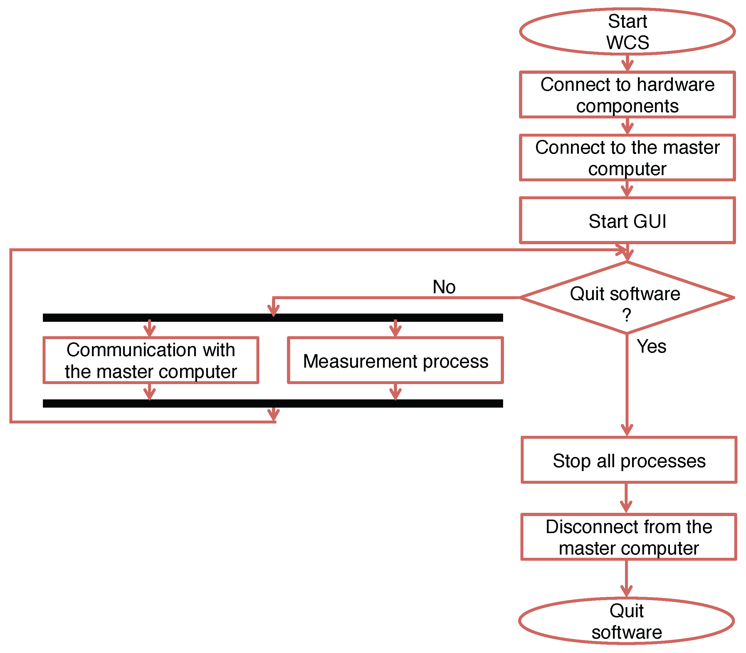
The WCS is software developed by DTU Wind Energy in the LabView environment that utilizes the aforementioned measurement process control. Essential software libraries, such as the MLE dll, and hardware drivers have been provided by Leosphere. A simplified flow diagram of the WCS is shown in Figure 4. The WCS is network-based application remotely configured by additional software residing on a physically-separated computer (master computer). There are two main loops in the software which run in parallel. One loop is handling the communication with the master computer, while the other loop is governing the measurement process.

The WCS user has substantial freedom in configuring the software, thus optimizing the LRWS measurement process to suit the needs of field campaigns. The software is configured by two ASCII files, the range gate file containing range information, and the motion program defining trajectory, laser pulse emission and pulse echoes acquisition. These two files are loaded in the measurement process loop and used to set all hardware components. For typical scanning strategies, such as LOS, PPI, RHI, DBS and time-controlled step-stare scans, the WCS contains subroutines, which automatically generate a set of files based on simplified user inputs. The files are generated and then loaded back to the WCS to have a record of previous configurations of the WCS. Furthermore, recording the configurations provides the means to run LRWSs independently of the master computer. More complex scanning strategies are manually described by the user, which needs to code the motion program, write the range gate file and submit them to an LRWS.

4. Forming a Multi-LiDAR Instrument

The long-range WindScanner system has been formed by adding an additional portable PC, which we refer to as the master computer, to the set of three LRWSs (Figure 5). The master computer coordinates the three LRWSs by:

• Configuring the WCS on each LRWS to execute certain scanning strategies
• Issuing the measurement start time
• Monitoring the LRWSs activities
• Intervening if necessary

Centralizing the coordination of multiple CDLs to the master computer significantly reduces the complexity of performing field campaigns and is necessary in order to achieve a strict synchronization among multiple CDLs.

4.1. Remote Sensing Communication Protocol

The master computer coordinates the LRWSs by exchanging network packets with them. This network communication between the master computer and the LRWSs has been described by the Remote Sensing Communication Protocol (RSComPro [40]). The RSComPro is an open application layer protocol [41], which defines:

• Commands sent from the master computer to the LRWSs
• The LRWSs actions in response to commands
• Answers to commands
• Alerts sent from the LRWSs to the master computer
• The structure of network packets that encapsulate commands, responses and alerts

The RSComPro exploits both the UDP transport protocol, for fast delivery of network packets to\from the master computer, and the TCP transport protocol, for reliable delivery of mission-critical network packets. The size of network packets is typically about one kilobyte, so that uninterrupted and fast coordination of LRWSs is possible even in the case of a mobile network, such as a 2G mobile network (i.e., GSM). In the most recent long-range WindScanner system deployments, a 3G mobile network was used [42].

4.2. Master Computer Software

The Master Computer Software (MCS) was developed by DTU Wind Energy in the LabView environment in accordance with the RSComPro. It is multi-platform software delivered as a light executable (5 MB). A simplified flow diagram of the MCS is shown in Figure 6. The MCS provides a Graphical User Interface (GUI) to design, execute and monitor field campaigns with the long-range WindScanner system (Figure 7). At a low level, based on the user inputs, the MCS generates, sends, receives, processes and displays the network packets.

The MCS is designed for remote instrument hardware monitoring, data storage and display, and it includes a set of automatic routines that handle alert states of LRWSs. The automatic routines are programmable and allow for the setup of automatic decisions in accordance with the input parameters (e.g., a change in wind direction triggers the change of a scanning strategy). Furthermore, the MCS is used for the assessment of static pointing accuracy of the LRWSs through the dedicated submodule CNR mapper [43]. Lastly, the MCS is responsible for keeping the LRWSs synchronized (see the following section). The MCS allows for the coordination of any reasonable number of remote LRWSs, as well as the coordination of other remote sensing instruments, the software of which is adapted for the network communication defined by the RSComPro [40,41].

5. Synchronization

In a multi-Doppler LiDAR system, the scanning trajectories will usually be synchronized in the sense that they will start and finish at the same time. The beams may well measure at different points in space during the scanning trajectories, for example dual PPI scanning of a horizontal plane. The data analysis nearly always entails forming averaged radial velocities at a number of points and then combining these and reconstructing the mean flow field from these averages. Failure to synchronize would greatly handicap the data analysis.

A special case of synchronization is when each trajectory is formed such that the acquisition of at least one pair of radial velocities is co-located at a special point of interest. This point can be stationary or it can move. Turbulence measurements nearly always require measurements of this type since it allows a time series of wind velocity to be reconstructed at the acquisition frequency.

In the case of the long-range WindScanner system, preconditions for attaining the LRWSs’ synchronization have been met with the time control of the LRWSs’ measurement process and accurate time information from the GPS-driven clocks. However, the asynchronization between the LRWSs can still be expected due to two factors that will be explained in the following section.

5.1. Asynchronization Factors

Windows 7, on which the WCS operates, is not a Real-Time Operating System (RTOS), and as such, it can introduce variability in the amount of time the execution of the sequential WCS actions takes. This results in the start time offset, which we define as the difference between the commanded and actual start time of a scanning strategy. The value of the start time offset is random; thus, it differs from one to another start of the scanning strategies. At best, the values of a few milliseconds have been observed.

Once the scanning strategy is started, the motion controller, which runs RTOS, controls the timing and execution of the scanning strategy. The motion controller phase and servo clocks’ signals control the timing of the scanner head and virtual stepper motor moves [38]. The source for the phase and servo clock’s signals is the crystal clock oscillator. The crystal clock oscillator frequency (20 MHz) has a finite accuracy of 50 parts per million (PPM). Due to this finite accuracy, the commanded time any action takes by the motion controller will lag or advance in the range of ±50 $\mathsf{\mu }$s every second of the scanning strategy execution.

Since the start of the scanning strategy can be delayed, and the time actions can progressively lag or advance throughout the execution of the strategy, we should expect that multiple LRWSs will drift apart if there is no intervention. Irrespective of the number of LRWS in the long-range WindScanner system, the maximum drift speed will be 100 $\mathsf{\mu }$s/s.

5.2. Asynchronization Confirmation

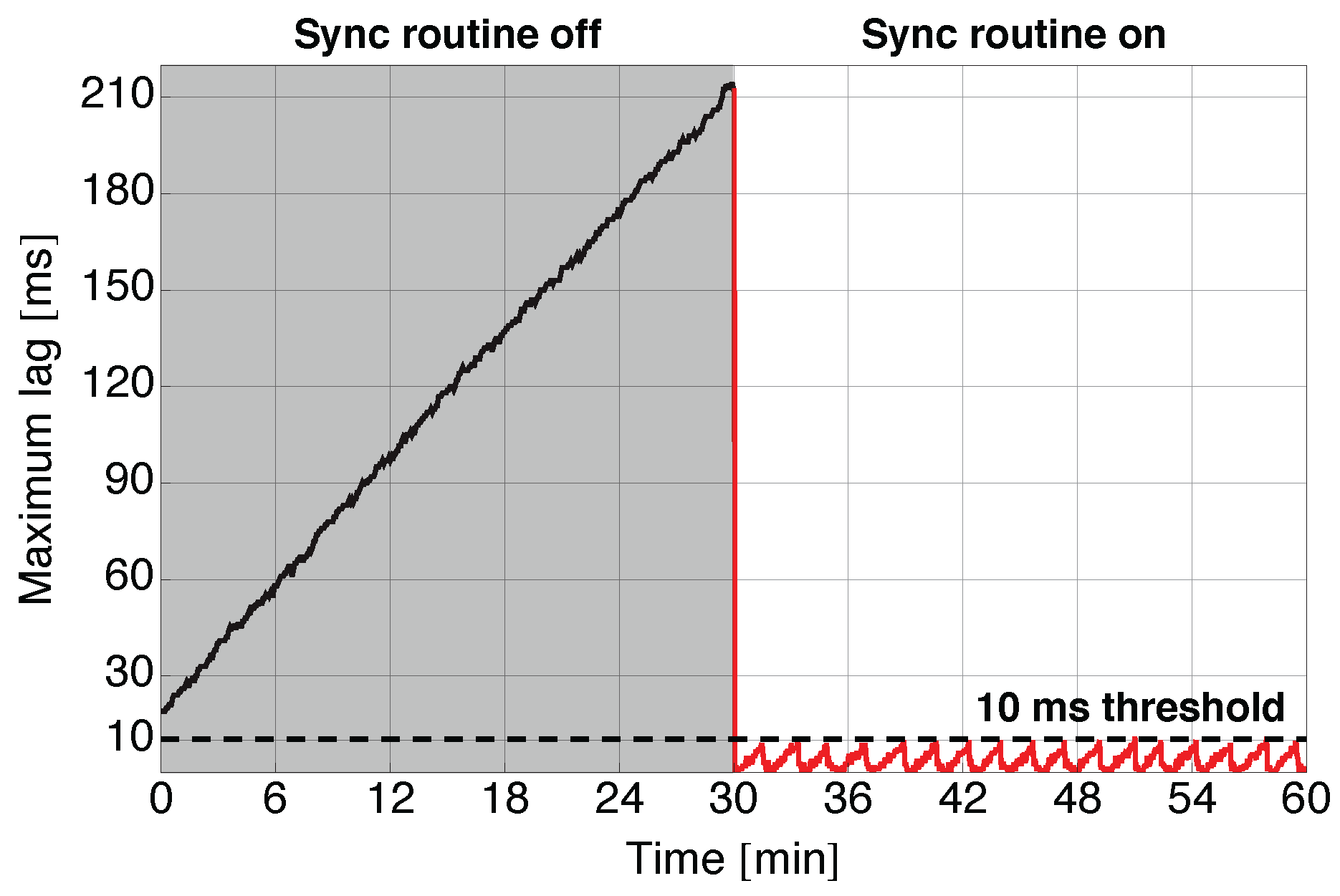
The asynchronization was first confirmed in an experiment where two LRWSs were configured to synchronously intersect beams at two points in the atmosphere. At each point of the intersection, radial velocity measurements were taken during the time of one second, while in between each intersection point, only the scanner heads were moving. Once the scanning strategies were started, we observed the start time offsets of 40 and 59 ms from the commanded start time; thus, the two LRWSs started the scanning strategy with a 19-ms difference. Throughout the execution of the scanning strategies, the LRWSs drifted apart (Figure 8). The maximum lag, which we define as the time difference when a radial velocity measurement took place at the ‘fastest’ and ‘slowest’ WindScanner in the system, was progressively increasing with the drift speed of 107 $\mathsf{\mu }$s/s. This result is slightly larger than the anticipated maximum drift speed.

5.3. Synchronization Concept

To keep the LRWSs synchronized, the sync routine has been developed. In this routine, the master computer monitors the maximum lag and interacts with the LRWSs when a particular maximum lag threshold is reached. The master computer sends “synchronize” commands to the LRWSs, the execution of which slows down the LRWSs that are advancing in comparison to the slowest LRWS.

Slowing down is achieved by adapting the motion programs to have an option that extends the commanded time of a scanner head motion when the WCS sends slow down requests to the motion controller. Another way of slowing down the fastest LRWSs is to include G-Code command G4 in the motion program that, when triggered by the WCS, puts the execution of the lines of the motion program code that follows on hold for the period of time set by the WCS. Typically, the scanner head motion from the last measurement point back to the first measurement point is extended, thus when there are no planned measurements, or the G4 command is executed right after the last measurement point, that is before the start of the next iteration of the same scanning strategy.

This synchronization concept with the G4 command was switched on 30 min after the start of the aforementioned experiment. In Figure 8, we can see that each time the threshold of 10 ms was reached (about every 90 s), the master computer was sending the synchronization commands to the fastest LRWS, which resulted in the reduction of the maximum lag to about zero ms.

6. Field Performances

The long-range WindScanner system has been operational since 2013, and it has been used in single-, dual- and triple-Doppler modes. To date, 12 measurement campaigns have been done with the system, and in this section, we will review several of them.

A system consisting of the three LRWSs was used to study the development of the internal boundary layer as the flow field makes a transition from the sea to the coast [44]. Furthermore, this study was used to validate the data quality of the retrieved wind vectors from the long-range WindScanner system by comparing them with the wind vector measurements made with a sonic anemometer mounted on a 20-m mast (reference mast). The experiment took place at Høvsøre [45]. A high correlation between the retrieved LiDAR and sonic anemometer horizontal wind speeds has been reported, whereas limitations in the vertical wind speed retrievals have been indicated. Primarily, the cause of the poorer retrieval of the vertical wind speed was attributed to the low elevation angles employed during the measurement process. The distance between the three LRWSs and the reference mast ranged from 60 m (one LRWS) to about 1 km (two LRWSs).

The system consisting of a single LRWS was used to experimentally validate a novel scanning strategy in measuring turbulence using a six-beam method [46]. Furthermore, this experiment took place at Høvsøre. As Høvsøre is a flat site with homogeneous and low vegetation, the assumption of the horizontal homogeneity of the flow is typically satisfied. The experimental results showed high accuracy of the horizontal wind speed acquired with a six-beam method (within 1% comparing to co-located cup anemometer measurements). Improved turbulence measurements in comparison to the VAD method were reported.

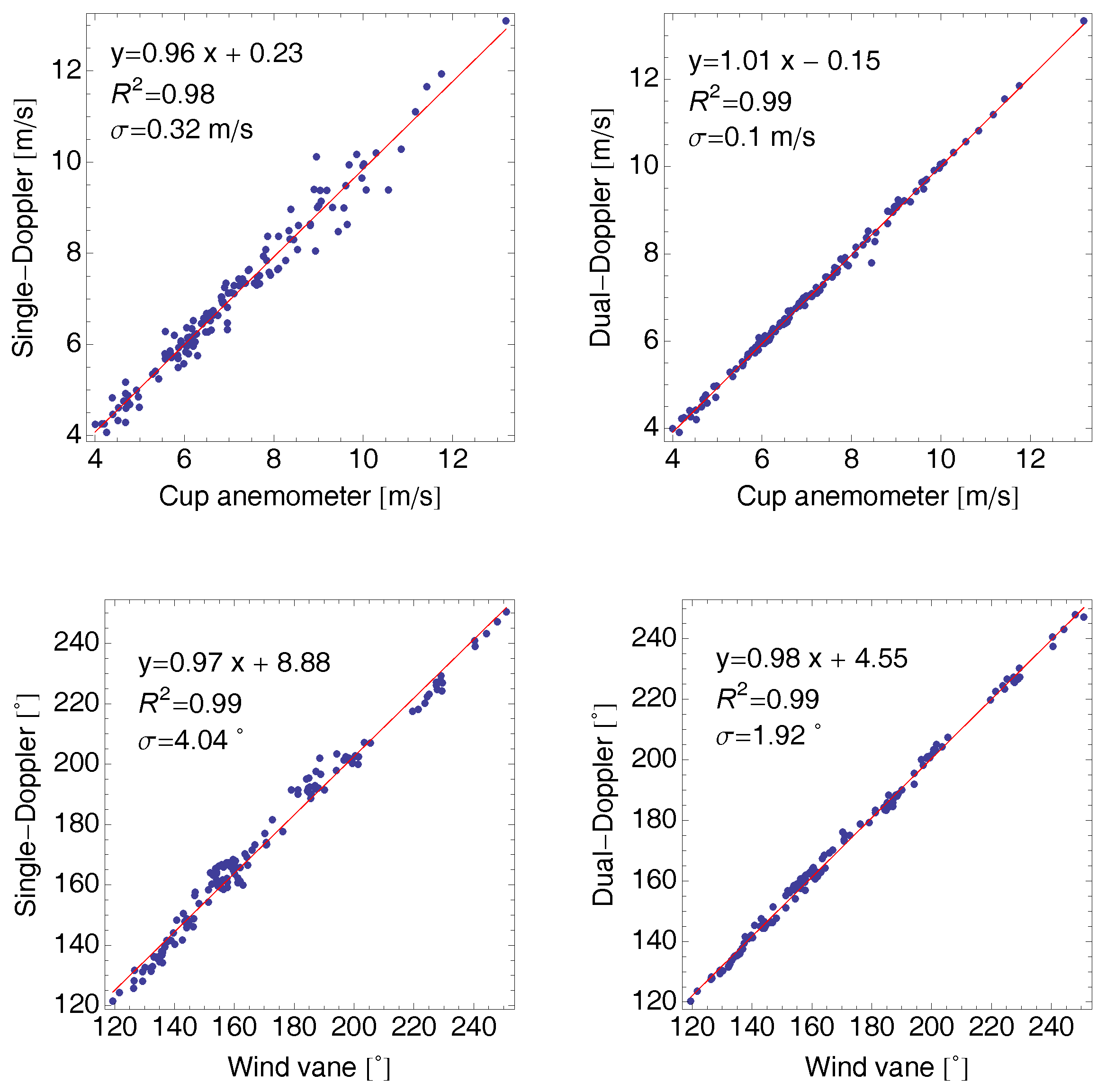
On the same site, the long-range WindScanner system with the three LRWSs was used for the comparison of single- and dual-Doppler setups for the retrieval of the horizontal wind speed and wind direction for flat coastal and near-shore sites [47]. In the dual-Doppler configuration, two LRWSs were configured to intersect the laser beams above a 116-m mast (reference mast), where a cup anemometer and wind vane are mounted. Since low elevation angles were used to direct the laser beams (<6${}^{\circ }$), the vertical wind speed could be neglected, and the horizontal wind speed and direction were directly resolved using two independent LOS measurement. At the same time, the third LRWS was configured to perform 60${}^{\circ }$ PPI scans (sector-scans) above the mast, where iVAP technique [12] was applied on the LOS measurements to retrieve the horizontal wind speed and wind direction. The distance between the three LRWSs and reference mast ranged from 1.1 km (one staring LRWS and one sector-scan LRWS) to 1.6 km (one staring LRWS). The horizontal wind speeds and wind directions retrieved in the single- and dual-Doppler configurations compared well with the measurements acquired with the top mounted cup anemometer and wind vane (Figure 9). Overall, the dual-Doppler results show generally less scatter in retrieving the horizontal wind speed and wind direction compared to the single-Doppler results. Nevertheless, the single-Doppler results indicate that single sector-scanning LiDAR seems to be a cost-effective solution for the flat coastal and near-shore wind resource assessment. However, it should be noted that due to the presence of the wind turbines at Høvsøre, only the single-Doppler retrievals acquired during the wind conditions in which the wind direction was between 118${}^{\circ }$ and 270${}^{\circ }$ were analyzed. For this range of wind directions, the flow was never orthogonal to the scanned sector, but roughly parallel to it. The sector-scan configuration, specifically an optimum sector size, has been further studied in [48] based on the collected data. The study indicated that in the case of the layout used in this experiment, the accuracy of the single-Doppler retrievals was deteriorating when the sector size was smaller than 30${}^{\circ }$. On the other hand, the accuracy of the single-Doppler retrievals did not differ significantly for the sector size from 30${}^{\circ }$ to 60${}^{\circ }$. The study proposed that an optimum sector size is in the range of 30${}^{\circ }$ to 38${}^{\circ }$.

This study was a prequel to a large experiment that was performed under the Reducing the Uncertainty of Near-shore Energy estimates (RUNE) project [49]. The RUNE project aims at improving meso- and micro-scale flow models’ predictions of near-shore energy estimates using the observations from the long-range WindScanner system. Currently, an in-depth data analysis is underway.

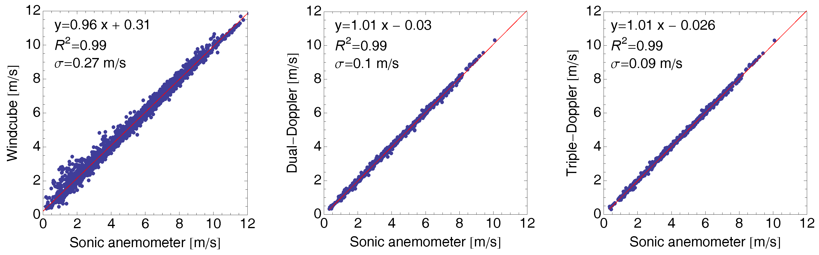
The previously-described campaigns were addressing wind fields measurements in flat terrain and offshore environments. Furthermore, the long-range WindScanner system has successfully tackled challenges in operating in remote and harsh environments, such as complex terrain. The long-range WindScanner system expanded by an additional three LRWSs from the ForWind institute (six LRWSs in total) was operated near Kassel in Germany (Kassel 2014 experiment, [50]). The aim of the Kassel 2014 experiment was to inter-compare multi-LiDAR and profiling LiDAR (Windcube V2) measurements against the mast measurements in complex and forested terrain [50]. The distance between the LRWSs and the reference mast ranged from 2 m up to about 3.7 km (see the details in [50]). The results confirmed that in complex terrain (inhomogeneous flow), wind speed measurements performed using intersecting multi-LiDAR beams are significantly more accurate than those from single CDLs. The horizontal wind speeds retrieved by the long-range WindScanner system operated in triple- and dual-Doppler mode showed excellent agreement (within 1%) with the measurements acquired by a sonic anemometer and low scatter (Figure 10). On the other hand, when the measurements simultaneously acquired by a standard Windcube V2 were compared to the sonic anemometer, this comparison showed a positive bias of the Windcube V2 measurements of the horizontal wind speed measurements and a much larger scatter. The Windcube V2 did not have the FCR algorithm installed. Therefore, the Windcube V2 acquired the wind speed and wind direction measurements that did not undergo modifications by the FCR algorithm. Furthermore, promising results of the turbulence measurements with dual- and triple-Doppler techniques were reported. Still, the challenge of acquiring vertical wind speed persisted. In this experiment, one LRWS was installed next to the mast and configured to vertically point the laser beam. However, due to the terrain topography and vegetation, it was difficult to align the vertical beam. This degraded the accuracy of the vertical wind speed retrievals. The Kassel 2014 experiment was the first experiment where the mobile architecture of the long-range WindScanner system [42] was implemented. The synchronization concept described in this paper worked well throughout the experiment. The LRWSs were synchronized within the 10-ms threshold set by the experiment’s operators. In a few instances, we had issues with the mobile network coverage, which occasionally resulted in some of the LRWSs getting disconnected from the master computer. While a shorter duration network fallout is not a significant problem since the LRWSs continue to run independently, a longer network outage results in loss of synchronization between the LRWSs.

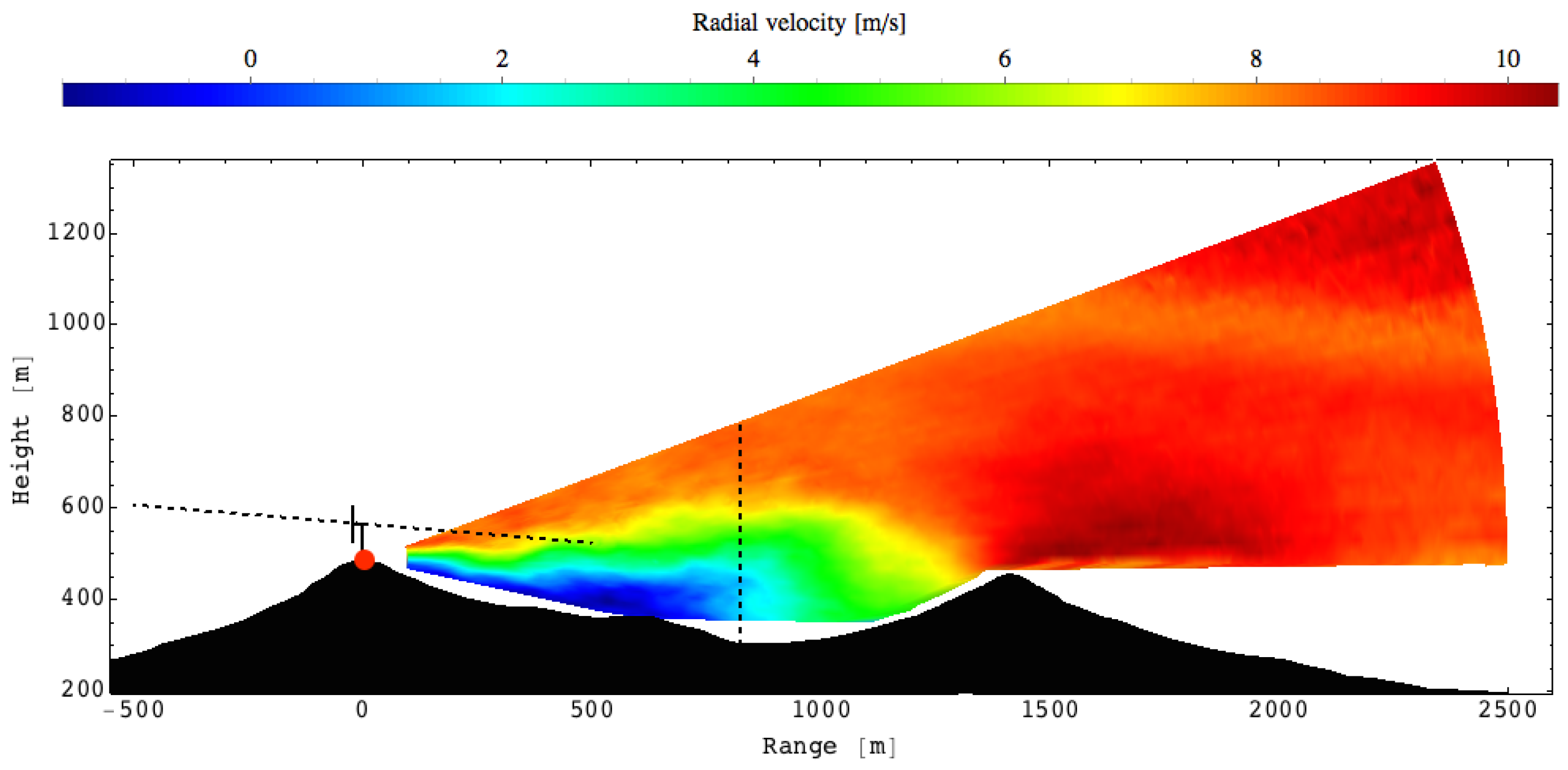
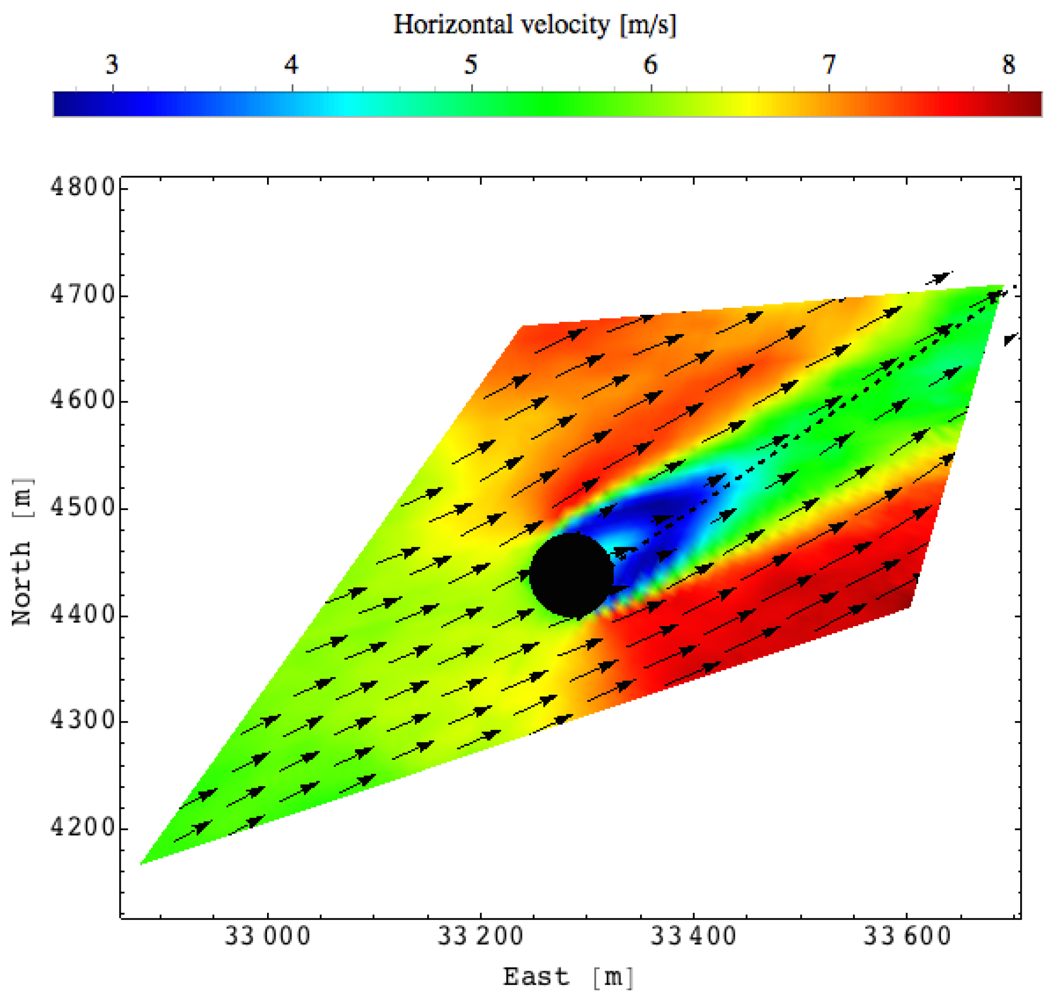
The previously-described campaigns were primarily intended to assess the accuracy of the long-range WindScanner system’s retrievals of the wind vector. Actual mapping of the wind flow with the system consisting of three LRWS was made during the Perdigão 2015 experiment [51]. This experiment was focused on creating a high-quality dataset of wind flow measurements for validation of wind resource estimation, wind turbine inflow and wind turbine wake models in complex terrain. The complex flow was measured in a great many points of interest, the number of which ranged from 50 up to 12,050. Several scanning strategies were designed and employed for the experiment [51]. An example of the acquired measurements are given in Figure 11 and Figure 12. The dataset is currently being used by several research groups for model validation [52,53].

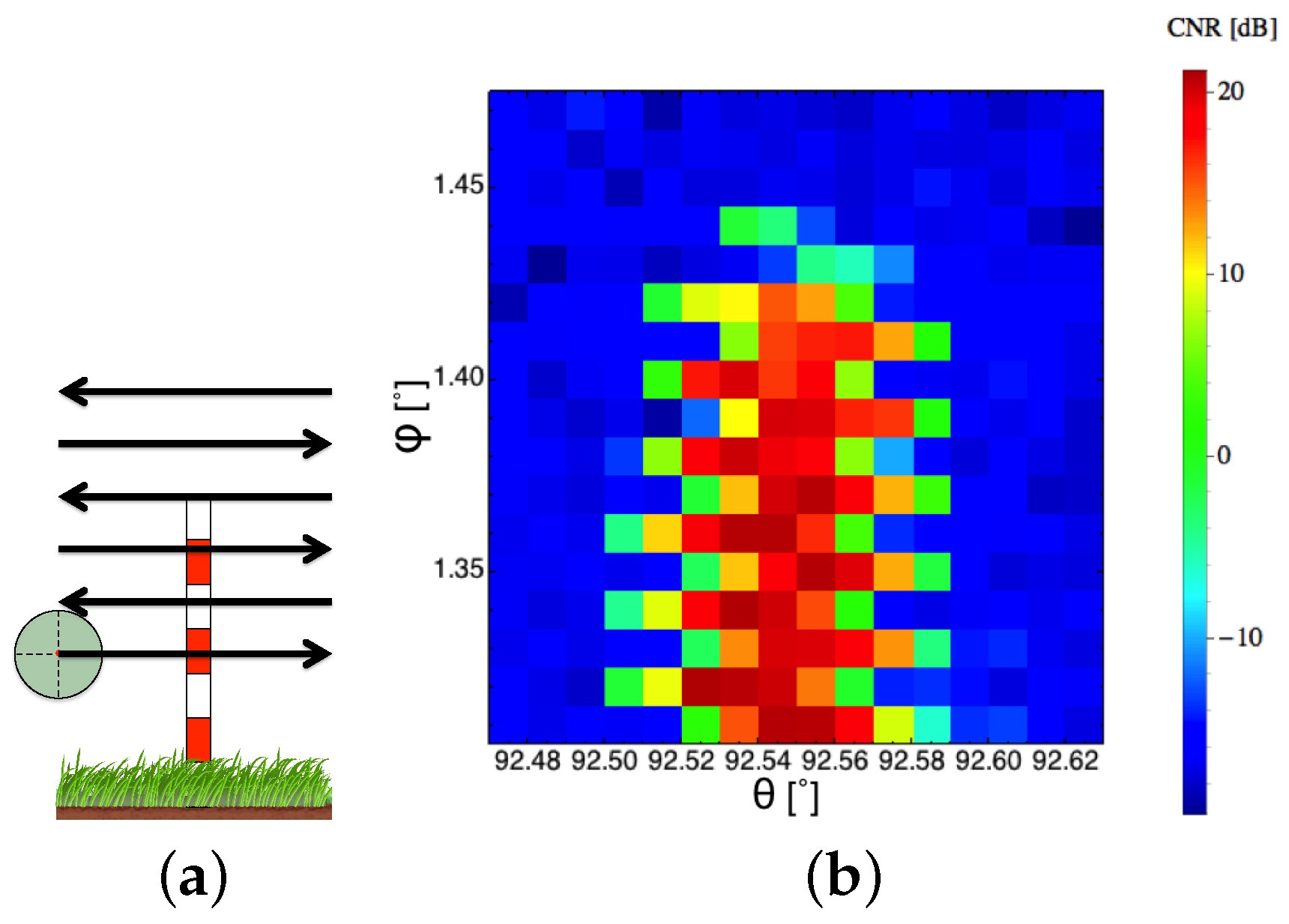
In the previous paragraphs of this section, we described the measurement accuracy of the long-range WindScanner system. Over the course of experiments, we have been investigating the pointing accuracy of the LRWSs. More specifically, prior to all measurement campaigns the static pointing accuracy of the LRWSs was tested. Usually, several thin survey poles and other landmarks of interest (i.e., hard targets) were mapped using the CNR mapper [43] and compared with the reference position readouts made by a theodolite and/or differential GPS. The CNR mapper creates a stack of PPI or RHI scans (TV scan), the execution of which steers the laser beam to map a hard target (Figure 13a). An example of the result generated using the CNR mapper is shown in Figure 13b. In this figure, we can see the CNR map of a 2 cm-thick survey pole located about 70 m from an LRWS made using a stack of PPI scans. The elevation angle of two consecutive scans differs for 0.01${}^{\circ }$, while the direction of the scanner head motion is opposite (Figure 13a).

The pole in Figure 13b is noticeable in comparison to the surrounding air since the intensity of the light backscattered by a hard target is orders of magnitude larger than the intensity of the light backscattered by aerosol particles. Each pixel in the map defines an area of 0.01${}^{\circ }$× 0.01${}^{\circ }$. We can observe in Figure 13b that the pixels in two consecutive rows are displaced. This is the result of backlash in the gearing mechanism. Namely, when switching from the one to the next PPI scan, the direction of the motion around the azimuth axis becomes reversed, introducing backlash. This means that even though the azimuth motor is turning, the scanner heads does not start to rotate until the clearance in the gearing mechanism is removed. The consequence is that the pole appears later in the CNR map comparing to the previous PPI scan. In the example shown in Figure 13b, the displacement of the pixels corresponds to the backlash level. In this particular example, the averaged displacement is equal to two pixels or 0.02${}^{\circ }$.

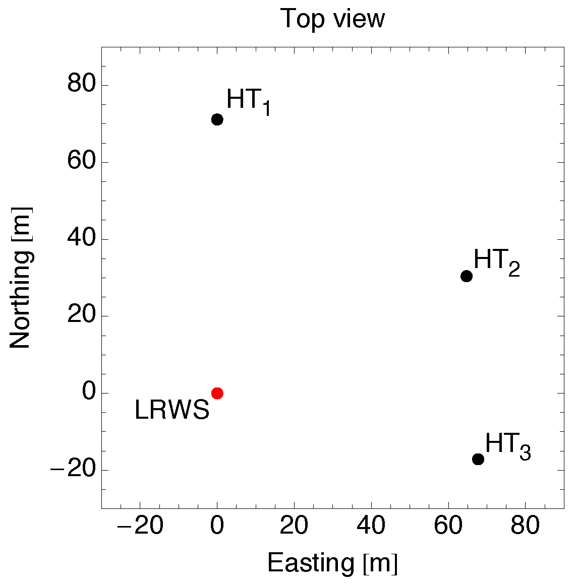
In Figure 14, an example of the layout for the static pointing accuracy test is given for one LRWS which was used during the Kassel experiment setup. The coordinate system in the figure is relative to the LRWS. Three survey poles were used in this test. The difference between the mapped positions of the survey poles and reference positions calculated using the read-outs from a multi-station (combination of theodolite and differential GPS) are given in

Table 4. Reference and mapped positions of landmarks (azimuth angle, θ; elevation angle, φ; distance, D).

	Reference			Mapped		Difference
Landmark	${\mathit{\theta }}_{\mathit{r}}$(${}^{\mathbf{\circ }}$)	${\mathit{\phi }}_{\mathit{r}}$(${}^{\mathbf{\circ }}$)	${\mathit{D}}_{\mathit{r}}$(m)	${\mathit{\theta }}_{\mathit{m}}$(${}^{\mathbf{\circ }}$)	${\mathit{\phi }}_{\mathit{m}}$(${}^{\mathbf{\circ }}$)	${\mathit{\theta }}_{\mathit{m}}\mathbf{-}{\mathit{\theta }}_{\mathit{r}}$(${}^{\mathbf{\circ }}$)	${\mathit{\phi }}_{\mathit{m}}\mathbf{-}{\mathit{\phi }}_{\mathit{r}}$(${}^{\mathbf{\circ }}$)
$H{T}_1$	0.04	−0.91	71.09	0.12	−1.10	0.08	−0.19
$H{T}_2$	64.97	0.99	71.48	65.04	0.88	0.07	−0.11
$H{T}_3$	104.32	3.08	70.04	104.40	2.95	0.08	−0.13
Mast top	91.04	5.87	3078.06	91.01	5.82	−0.03	−0.05

. The positions are expressed in terms of the coordinates of the spherical coordinate system, the origin of which coincides with the LRWS scanner head. The averaged difference between the mapped and references positions is 0.08${}^{\circ }$ and −0.14${}^{\circ }$ for the azimuth (θ) and elevation (φ) angles, respectively. In this example, the difference between the mapped and references positions for each survey pole compares well with the mean difference. 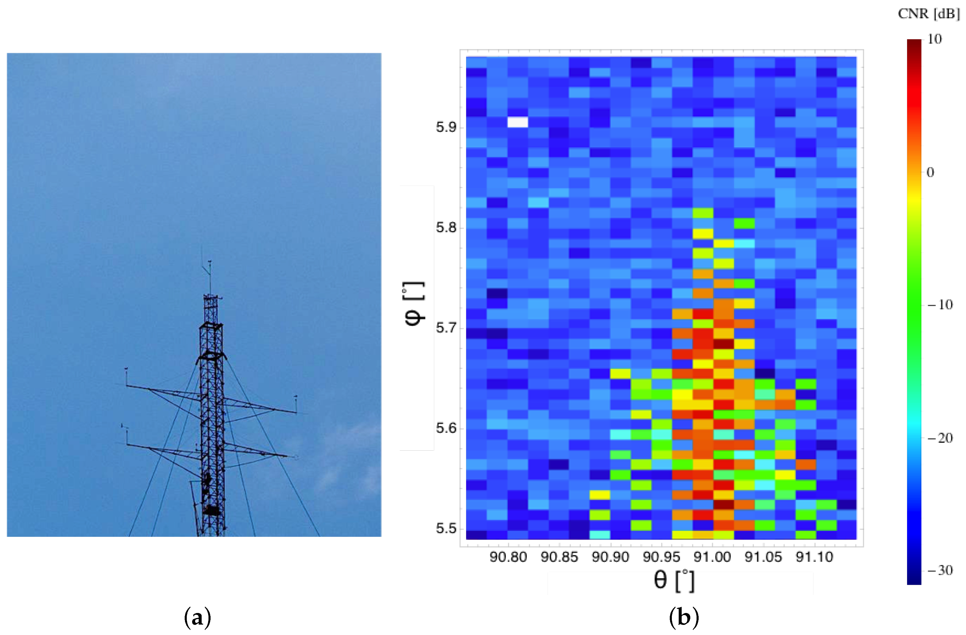The variation in the mean difference (maximum −0.05${}^{\circ }$) for the elevation angle is typically attributed to imperfect leveling, whereas the mean difference represents the home position offset of the scanner head. Commonly, the home position offset is introduced to the motion controller, which repositions the scanner head to the new home position. Following this step, a distant control landmark is mapped to check if the static pointing accuracy is really improved. In this example, we mapped the top of the mast located approximately 3 km from the LRWS (Figure 15). Based on the results given in Table 4, we can see that the difference between the mapped and reference position is −0.03${}^{\circ }$ and −0.05${}^{\circ }$ for the azimuth and elevation angles, respectively. Therefore, indeed by introducing the home position offsets, the static pointing accuracy has been improved. If the variation in the mean difference is significant, the variation is used to calculate how much an LRWS is pitched and rolled. Based on these results, either we attempt to improve the leveling of the LRWS, or we account for the pitch and roll offsets when coding the motion programs.

The above-described test of the pointing accuracy represents a part of our standard procedure for setting up field campaigns with the long-range WindScanner system. In all of our tests, we found that the averaged error in laser beam pointing was about 0.05${}^{\circ }$; the averaged backlash was approximately 0.025${}^{\circ }$; while by mapping the same hard targets several times, we found that the averaged repeatability of the scanning strategy was well within the CNR mapper resolution (i.e., 0.01${}^{\circ }$). Recently, for the purpose of studying the static pointing accuracy in more details, we performed a study where a large number of landmarks was employed and mapped. The results of this study will be described in a separate publication.

7. Discussion: How to Make an Even Better Long-Range WindScanner System

We have developed a new pulsed scanning CDL, the LRWS. The LRWS has been engineered with novel measurement process control. The measurement process control is not only tailored for pulsed scanning CDLs. In fact, this methodology is applicable to the development of CW scanning CDLs, such as our short-range WindScanners [34], and pulsed scanning Doppler radars, as these instruments also perform similar fundamental processes like the above-described fundamental processes of pulsed scanning CDLs. A CW scanning CDL emits and focuses a CW laser beam at a single range, steers the laser beam, acquires the backscattered light from a single range and processes the backscattered light to provide LOS retrievals. In the case of pulsed scanning Doppler radars, the only essential difference is that radars emit radio-wave pulses instead of laser light pulses. Both CW scanning CDLs and scanning Doppler radars require a tight synchronization among their fundamental processes for the same reasons as pulsed scanning CDLs do (i.e., knowing when and where information on the flow is retrieved).

In accordance with the measurement process control, the WCS has been developed. The measurement process control and the WCS provide users significant freedom in configuring the long-range WindScanner. Users are able to set up arbitrary and time-controlled scanning strategies. Arbitrary and time-controlled scanning strategies are essential for realizing a synchronized multi-LiDAR instrument. LRWSs are the first and, so far, the only pulsed scanning CDLs that can perform this type of strategy. However, even though the WCS has a dedicated module for automatic scanning strategies generation, this module can only generate a limited number of scanning strategies. The arbitrary strategies are manually parametrized, and this process requires solid knowledge of the kinematics of the scanner head and how the motion controller executes the kinematic routines. We are currently working on an extension of the aforementioned module that will simplify and automatize the generation of arbitrary and time-controlled scanning strategies.

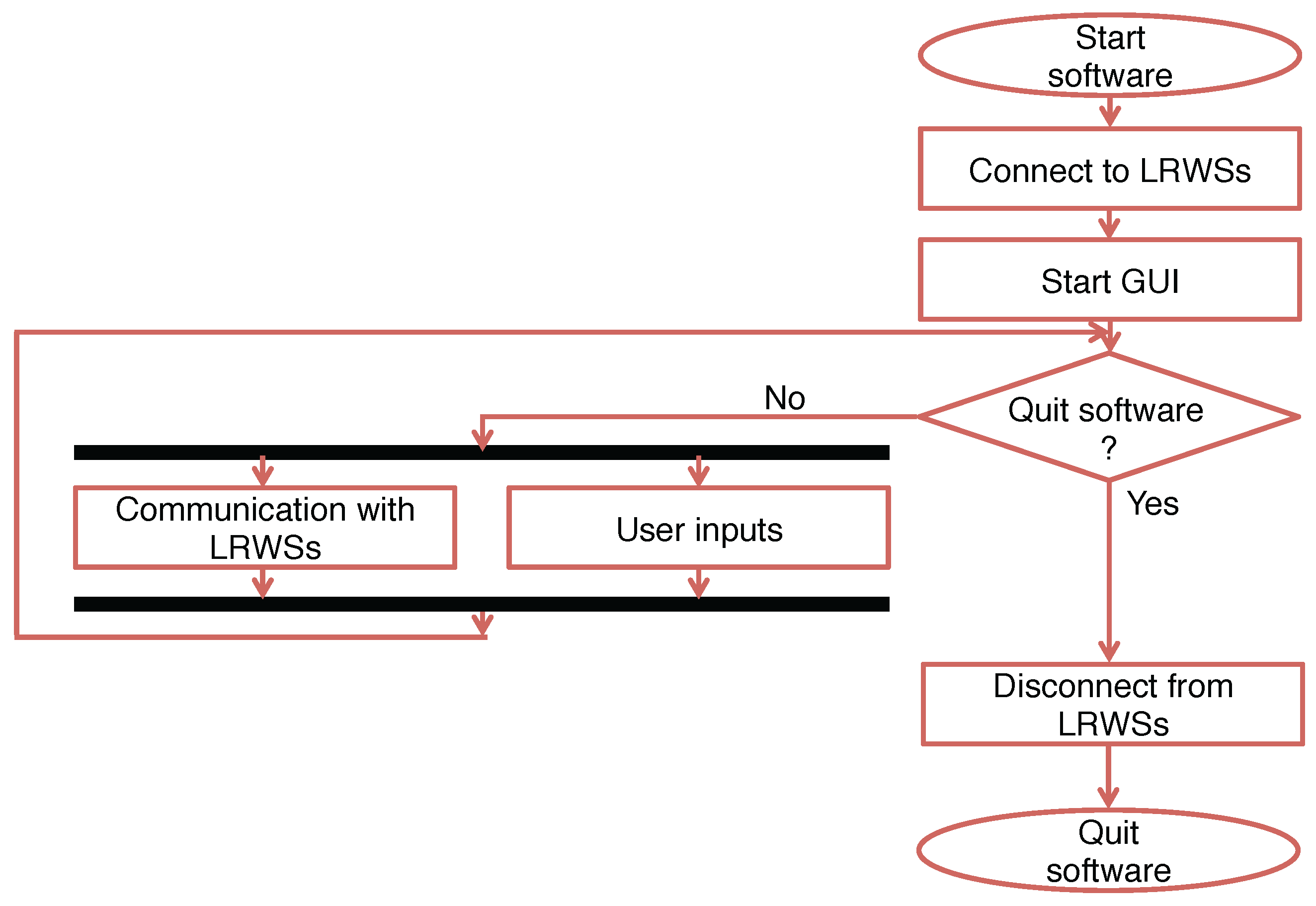
We have formed the long-range WindScanner system, a multi-LiDAR instrument, by employing several LRWSs and wirelessly coordinating them using a remote master computer. Since the coordination is achieved by an exchange of approximately 1-kB network packets, a mobile network can be adopted for the communication between the master computer and LRWSs. An effective software solution for synchronizing LRWSs in the long-range WindScanner system has been devised. The synchronization mechanism can be used using both wired and wireless network types, including 2G networks. Network delays are not critical since the GPS times are measured locally. In this respect, there is virtually no limitation in the separation among the LRWSs. It has been shown that this solution can keep the maximum lag in the long-range WindScanner system below 10 ms. Even though the software solution is based on slowing down the fastest LRWSs in the system and, thus, a reduced number of samples over the measurement period should be expected, it can be shown that the reduction is negligible (0.02%). However, the software solution requires that the network connection between the LRWSs and the master computer is maintained over the course of measurements. If the network connection is lost, the LRWSs will drift apart, and their synchronization will be lost. However, as the LRWSs can operate without the master computer if the connection is lost, they will continue to loop on the last scanning strategy configuration. Therefore, the LRWSs will continuously acquire measurements until they are manually stopped. In the case of the permanent loss of the connection between the LRWSs and master computer, a simple solution would be to preload the LRWSs with a set of scanning strategies and to configure them to loop on the preloaded configuration. Still, due to the current hardware limitations, the LRWSs will eventually drift apart (lose synchronization). This issue can be solved if the motion controllers are provided with more accurate and stable clocks instead of the existing crystal clock oscillators. Oven-controlled crystal oscillators or atomic clocks can be the substitute for the existing crystal clock oscillators. Another alternative would be to make modifications of the WCS, such that this software automatically keeps the measurement process synchronized according to the previously-established time schedule. In this case, the WCS would need to be provided with the information about the exact timing when each measurement will take place. By monitoring the actual time when measurements occurred, the WCS would be able to calculate whether the measurement process is advancing or lagging compared to the planned time schedule. The above-described synchronization concept can be used either to slow down or speed up the measurement process and keep it synchronized to the established schedule. In this way, the LRWSs will be synchronized without the master computer. Preferably the OS of the LRWSs should be replaced by an RTOS, since this would allow more control over the timing of the software loops.

We have demonstrated high accuracy of the horizontal wind speed measurements with the long-range WindScanner system in all terrain types. Specifically, we have shown that by operating the long-range WindScanner system in a multi-Doppler mode, it is possible to eliminate single LiDAR errors in complex terrain. However, the retrieval of the vertical wind speed remains a challenge. This component of the wind vector cannot be accurately retrieved if low elevation angles are employed. If high elevation angles are used, experimenters have to be careful about the pointing accuracy. On the other hand, assessing the pointing accuracy of the vertical staring CDL is another challenge that needs to be tackled.

The topic of the pointing accuracy is complex, and it deserves more attention by the wind energy community. We are actively working on understanding the pointing error sources and improving the pointing accuracy. We strive to achieve an averaged pointing error lower than 0.01${}^{\circ }$. We have investigated the static pointing accuracy and proposed a method for how this accuracy can be assessed. To date, the impact of the dynamics of the LRWSs on the pointing accuracy has not been addressed.

While testing and operating the LRWSs, we encountered several issues with the hardware design. The chassis of the LRWS’s casing was suspended on springs, resulting in tilting of the chassis as the scanner head and, hence, the mass center moved. This tilting causes the beam position to move, and it is detrimental to the beam pointing accuracy. By strengthening the casing-chassis connection and, thus, bypassing the springs, this issue was solved. During the operation of the LRWSs in a warm climate (∼40 ${}^{\circ }$C), particularly around noon, the air-conditioning system was not able to cool down the internal parts of the LRWSs, which forced us to stop measurements for several hours. This issue is probably a result of insufficient thermal isolation of the LRWSs and ill-designed air flow through the LRWSs. The short-term solution to tackle this issue is to build shades for LRWSs, which can be simple tents covering a portion or the whole of the LRWSs. Refurbishing or redesigning the casing would be a better long-term solution.

Several other reasons go in favor of redesigning the casing. During the operation of the LRWSs in a wet, humid and cold climate, it is necessary to replace desiccants every several weeks. Otherwise, humidity starts to build up on the internal face of the scanner head glass window, which impacts the measurement range. A heated window could be the solution to this issue. From the kinematic design perspective, the LRWSs should only have three feet, where each foot has only two contact points with the surface where LRWSs are installed. This would give a sufficient number of contact points to attain a kinematically-constrained system and prevent the residual motion of an LRWS. Currently, the LRWSs have eight feet, and thus, we have an over-constrained system, which makes leveling of the LRWSs more complex, can deform the LRWSs and leaves room for residual motion.

Similarly, we are considering redesigning the scanner head, for several reasons. The scanner head positions are acquired from the motor encoders, which do not necessarily correspond to the actual position of the scanner head due to the mechanical imperfections of the gearbox components and the presence of backlash. In [54], we showed that the pointing errors caused by the motor encoders’ read-outs can be up to 0.1${}^{\circ }$. We devised a solution to this issue in [54] by mapping the mechanical imperfections with a temporary set of encoders located on the scanner head and storing this information as a look-up table in the motion controller. Even though this solution provides a significant improvement in the pointing accuracy (errors reduced up to five-times), due to the gear-box wear and tear, the look-up table would need to be regularly updated. Despite the fact that this process can be automatized, it is still time-consuming (mapping of imperfections and backlash per one LRWS takes several days). The most appropriate solution is to have encoders directly attached to the scanner head (rather than on the motor shaft on the other side of the gear-box). However, due to the scanner head design, this approach will not eliminate backlash, but only reduce it. Backlash can be only eliminated by removing the gearing mechanism. This is only possible if a direct-drive scanner head is developed. Our intentions are to develop a new casing and direct-drive scanner head.

8. Conclusions

In this paper, we presented the long-range WindScanner system, a multi-LiDAR instrument, which represents a potential alternative for many tall meteorological masts. We demonstrated the ability of the system to acquire highly accurate wind speed measurements and to map wind flow in great details. Over a short time period, the long-range WindScanner system has become an attractive instrument for wind energy and atmospheric research. It has been widely used since 2013, and it has been selected as an important instrumentation for the New European Wind Atlas (NEWA) project. The NEWA is an ERANET+ project, which is funded by the European Commission and nine national funding agencies. In the future, we expect to have frequent and extensive campaigns with the long-range WindScanner system that will realize the full potential of the developed instrument. Furthermore, we will continue to work on improvements of the long-range WindScanner system that will make the instrument more robust, accurate and easier to use.