Self-Calibration Method Based on Surface Micromaching of Light Transceiver Focal Plane for Optical Camera

Abstract

In remote sensing photogrammetric applications, inner orientation parameter (IOP) calibration of remote sensing camera is a prerequisite for determining image position. However, achieving such a calibration without temporal and spatial limitations remains a crucial but unresolved issue to date. The accuracy of IOP calibration methods of a remote sensing camera determines the performance of image positioning. In this paper, we propose a high-accuracy self-calibration method without temporal and spatial limitations for remote sensing cameras. Our method is based on an auto-collimating dichroic filter combined with a surface micromachining (SM) point-source focal plane. The proposed method can autonomously complete IOP calibration without the need of outside reference targets. The SM procedure is used to manufacture a light transceiver focal plane, which integrates with point sources, a splitter, and a complementary metal oxide semiconductor sensor. A dichroic filter is used to fabricate an auto-collimation light reflection element. The dichroic filter, splitter, and SM point-source focal plane are integrated into a camera to perform an integrated self-calibration. Experimental measurements confirm the effectiveness and convenience of the proposed method. Moreover, the method can achieve micrometer-level precision and can satisfactorily complete real-time calibration without temporal or spatial limitations.

1. Introduction

High-resolution earth observation applications are essential in many fields, such as mapping, environment monitoring, and resource exploration. Such applications require high-resolution images and high-accuracy image positioning determinations [1,2,3]. However, high-accuracy and high-resolution optical imaging payloads need high attitude control precision, orientation, and transfer matrix of attitude [4,5,6,7]. The imaging payloads’ positioning accuracy determines the spacecraft performance, which is crucial for completing space missions. The GeoEye-1 satellite can collect panchromatic imagery with a resolution of 0.46 m and multispectral imagery with a resolution of 1.84 m; the system can also precisely locate an object within 5 m of its true location on the surface of the Earth with CE90 (Circular Error of 90%) [8], owing to the high-performance electro-optical camera developed by the International Telephone & Telegraph Space Systems Division [9]. The Pleiades-1B can acquire panchromatic (0.5 m) and multispectral (2 m) images with high geo-location accuracy (3 m @ CE90) and high resolution [10]. The system also employs a push-broom imaging concept [11]. NAOMI [12] is a product line of high-resolution optical cameras applied to SPOT-6 satellite and is based on the same telescope concept implementing one or several focal plane units in the same camera. The high-accuracy space smart payload system integrated with attitude and position (SSPIAP) can provide high resolution (0.5 m) and accurate location (3.7 m @ CE90) of images [13]. The system also integrates a high-resolution remote camera and miniature attitude- and position-sensitive devices, such as star tracker, micro-electro-mechanical system gyroscope, and global position system, into a new smart payload system. Inner orientation parameter (IOP) calibration is a prerequisite for image position determination of a camera. Given that remote sensing optical camera is much needed for high-accuracy position determination, its accuracy calibration must be high.

To complete the high-accuracy positioning of remote sensing camera, high imaging quality and high calibration accuracy of IOPs are needed. Numerous technologies have been proposed to improve the imaging quality of remote sensing cameras [14,15]. Specifically, a special optical hardware, such as wave front sensor [16], can determine the quality of wave fronts in front of detector array to correct dynamic optical aberrations that blur images. Advanced technologies can ensure high imaging quality for remote sensing cameras. Camera calibration methods have been proposed for different applications, such as IOP calibration methods for space optical camera [17,18,19,20,21,22,23,24,25]. Furthermore, laboratory measuring angle methods are widely used for IOP calibration of remote sensing cameras [26,27,28,29,30,31]. In this type of simple and micrometer-level calibration method, an uncalibrated optical camera is placed on a precision turntable in capturing the parallel lights of star points emitted by a collimator. Computer vision techniques [14,32,33] are used for camera calibration based on three dimensional (3D) coordinates of several given and image points; this type of method uses multiple views to calibrate intrinsic parameters, distortions, and image deformations. In 2001, multiple two dimensional (2D) diffraction grids are generated using crossed-phase diffractive optical elements [34]. The equally spaced dots can be used to calibrate wide-angle geometric cameras for photogrammetry. Moreover, these methods can be precisely calibrated in a laboratory; however, they may drift to a large degree because of vibration during complicated launches and on-orbit working conditions. Furthermore, laboratory calibration approaches generally need a calibrated reference object. To mediate this problem, several self-calibration methods that do not require a calibrated reference object have been developed for calculating IOPs [35,36,37,38,39,40,41]. Self-calibration methods can use unfamiliar scenes and motions to calibrate a camera; moreover, these methods use constraints among the system parameters for calibration. Nevertheless, these self-calibration methods exhibit computational complexity, heavy computation, and nontrivial solutions of equations. Moreover, calibration accuracy cannot be guaranteed and its robustness is low.

Traditional methods for on-orbit calibration of remote sensing cameras use ground control point (GCP) or stars control point (SCP) methods [42,43]. However, the availability and access to GCPs is sometimes difficult. Moreover, operational SCP implementation is highly restrictive because acquiring star images wastes a long orbit portion before completing the attitude change of a space camera pointing to between Earth and space. Therefore, self-calibrating bundle adjustment is ideal for mediating control point limitations for on-orbit camera calibrations [44]. Lichti et al. [45] compared three geometric self-calibration methods for ranged cameras, and the self-calibration bundle adjustment is found to be slightly superior. However, the self-calibrating bundle adjustment method presents long computation times [46]. Moreover, 180° satellite maneuvers have been used to calibrate on-orbit cameras. Self-calibrating bundle adjustment needs a standard ground calibration field [47]. Delvit et al. [48] proposed an auto-reverse method during the commissioning phase. This method is efficient and does not require external reference data; however, its operational implementation is highly restrictive because acquiring a same-site image pair wastes along orbit portion before completing the alignment to ground projection of scan-line on ground velocity. Therefore, existing on-ground and on-orbit methods present common characteristics with the aid of external targets and are limited by space and time.

We develop an efficient self-calibration method for optical cameras. The proposed method considers the temporal and spatial limitations when conducting the calibration function based on surface micromachining (SM) of light transceiver focal plane. This method is expected to be highly accurate, easy to operate, require few auxiliary equipment, and replicate real orbit conditions. The proposed auto-collimating self-calibration method is based on a bi-plane dichroic filter element and an SM point-source focal plane (SM-PSFP).The on-orbit camera can perform integrated self-calibration without temporal and spatial limitations and is therefore a potential calibration standard. Moreover, this method can verify the functions of the on-orbit status of optical camera and can be used on-ground and on-orbit. The rest of the paper is organized as follows. The principle of the proposed method is introduced in Section 2 and Section 3, and the experimental results are presented in Section 4.

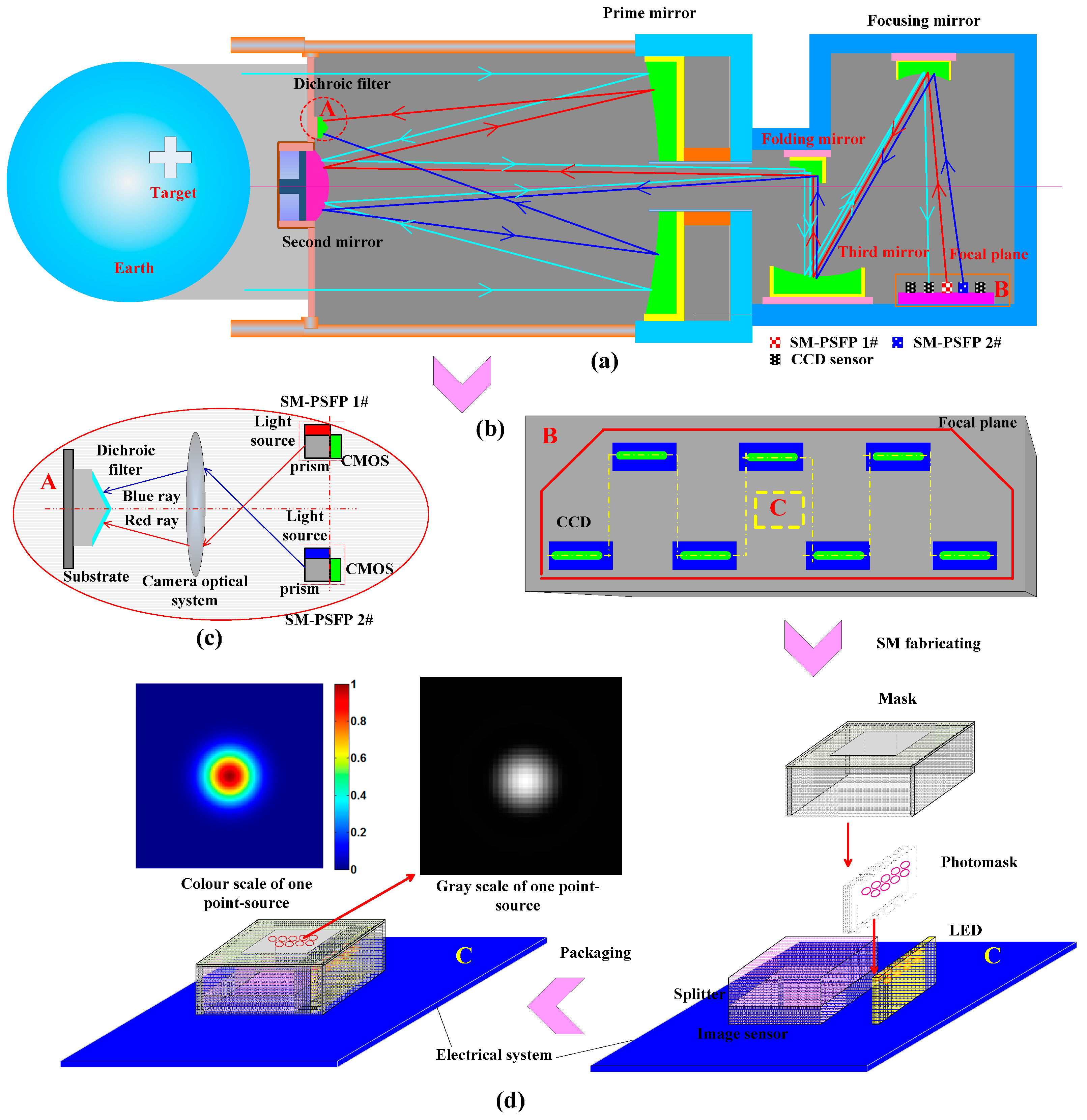
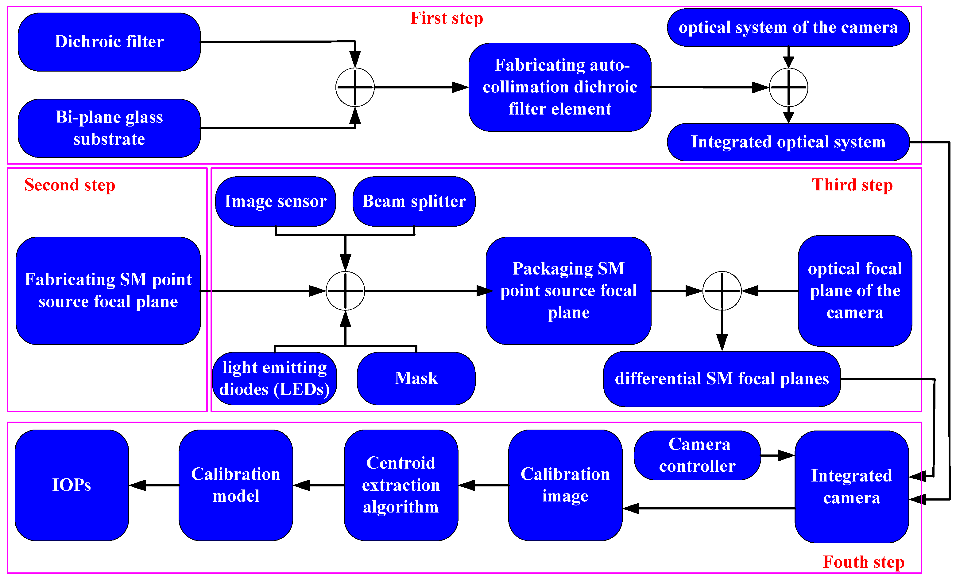
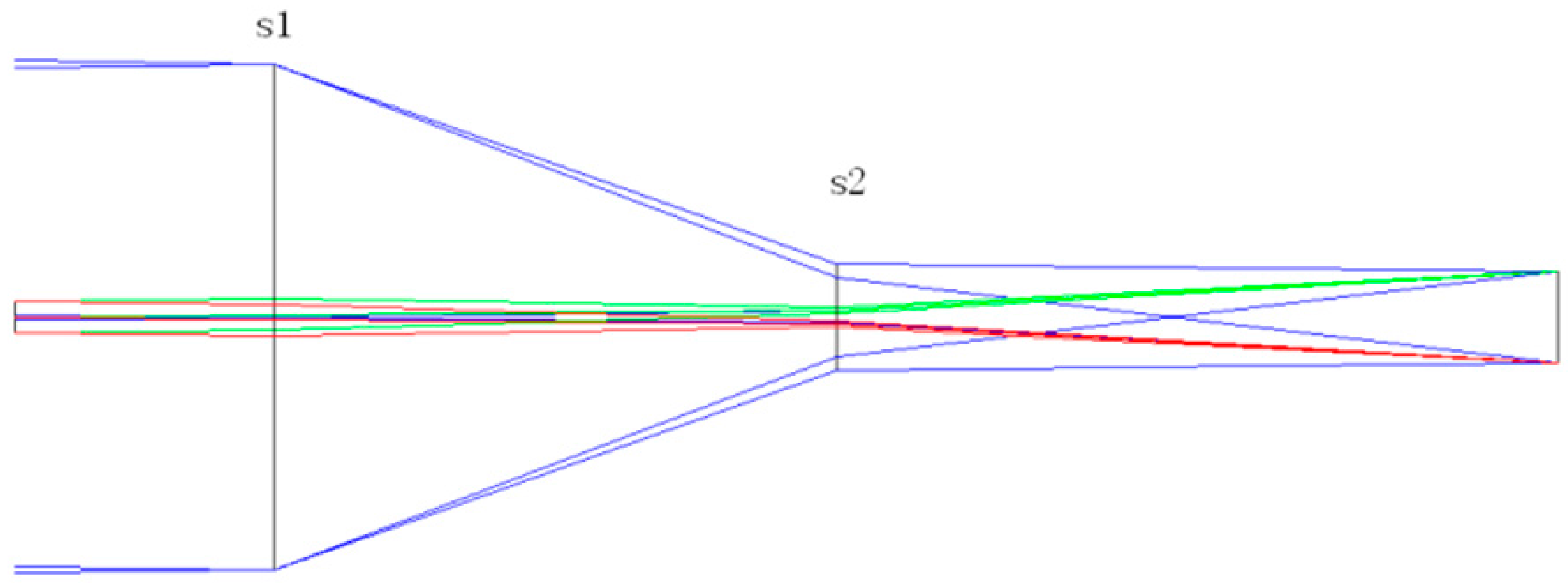
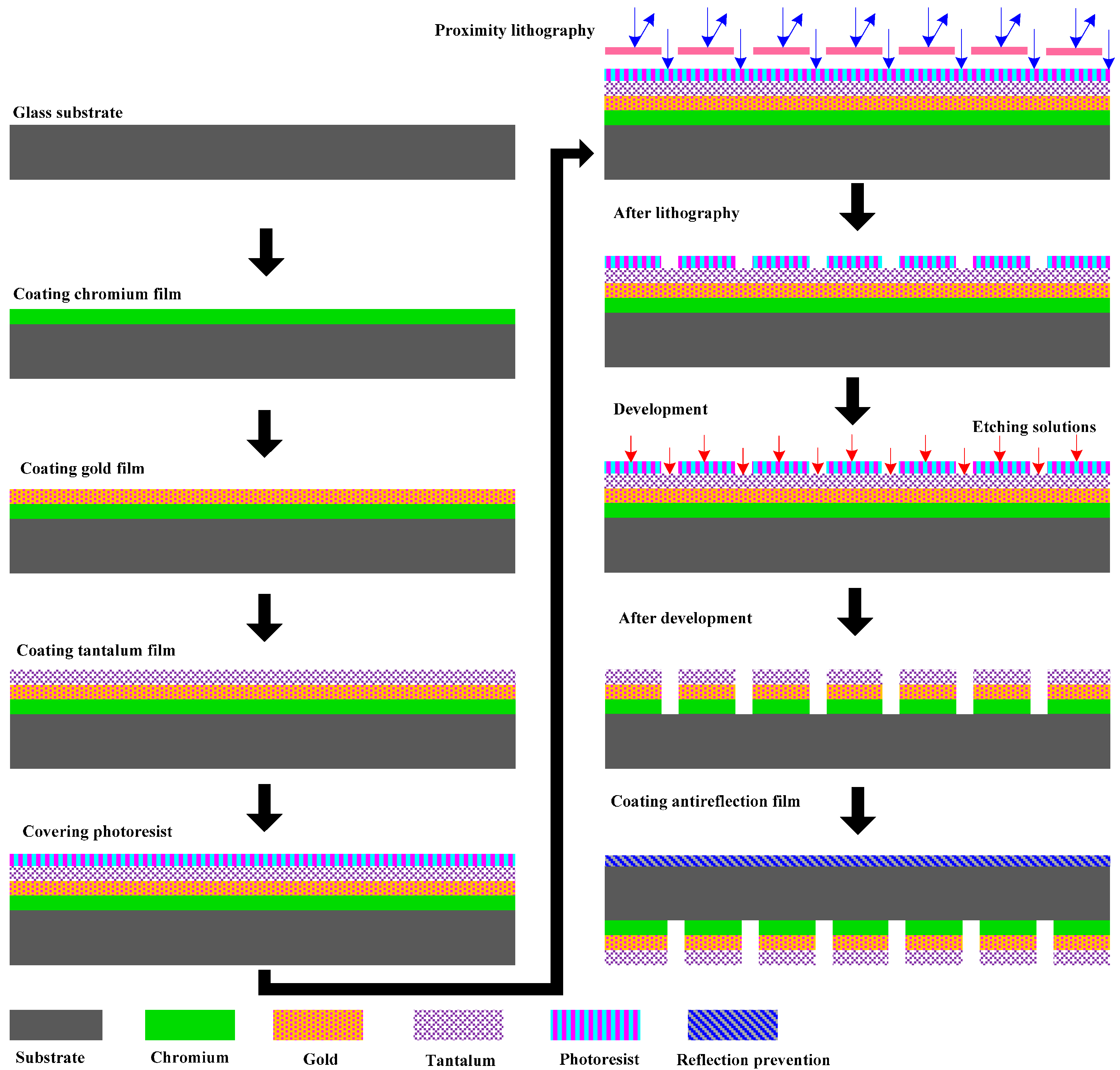
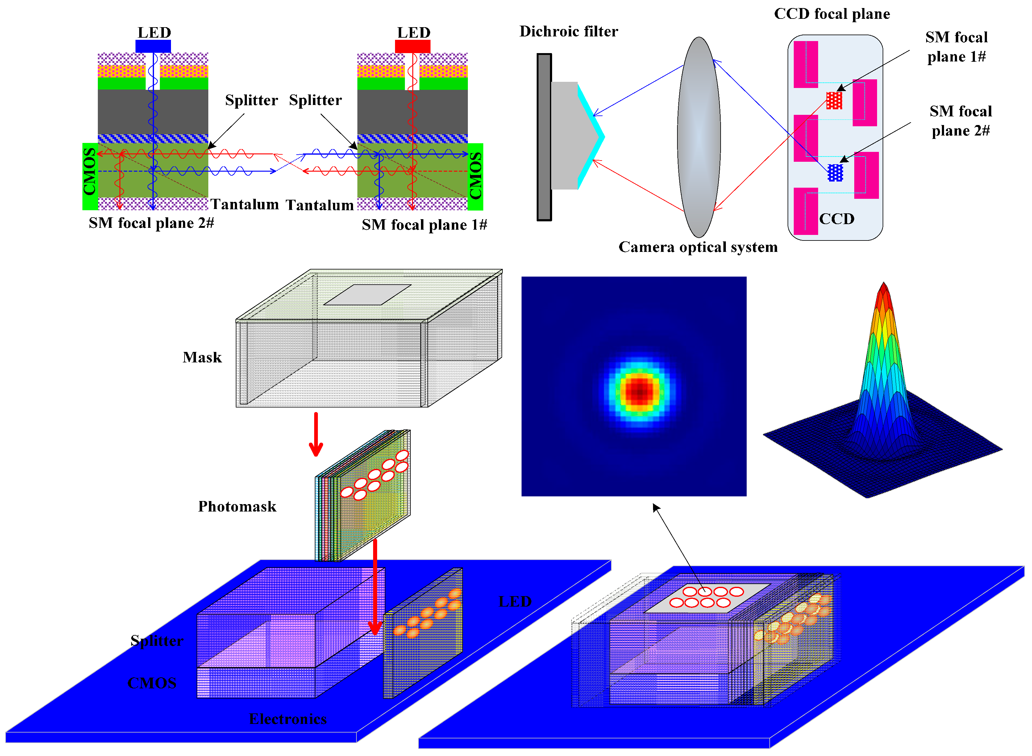
2. Proposed Self-Calibration Method

Positioning without GCPs is among the key technical problems for remote sensing photogrammetry. The IKonos-2 satellite can reach a positioning accuracy of 15 m without GCPs [49]. The WorldView-2 satellite can reach a positioning accuracy of 6.5 m without GCPs [50]. The GeoEye-1 satellite can provide a positioning accuracy of 4 m without GCPs [51]. The SSPIAP also adopts a positioning method without GCPs and requires a positioning accuracy of 5 m. Given that a camera generally uses forward and back-looking images to complete the digital mapping, the geometric performance of the camera must be accurate. To extract highly accurate topographical information from two overlapping strips of images, a camera must provide highly accurate IOPs. After adjusting the optical camera, the IOPs deviate from the ideal values specified by the design, manufacture, and assembly [52,53,54]. Therefore, accurate IOP calibration is necessary. The positioning accuracy (without GCPs) of a camera mainly depends on the accuracies of satellite station positioning, attitude measurement, image point measurement, and IOP measurement. Moreover, the error distribution of a remote sensing camera is obtained by the positioning algorithm. Without GCPs, the error distribution equation can be built based on the position of homologous pixel points of forward- and back-looking images, IOP, and a series of coordinate transforms from camera to ground. The error distribution can generally be divided into two aspects: (1) camera imaging with accuracy depending on pixel point measurement error and IOP measurement accuracy; and (2) position and attitude accuracies at forward- and back-looking imaging times. Combined with device performance of satellite, error distribution equations can calculate the optimal error distribution. For example, a positioning accuracy of 5 m can obtained by a camera if the distribution of its primary errors exhibits the following characteristics: (1) an attitude determination accuracy within 10′′ (angular seconds); (2) a precise orbit determination within 0.2 m; (3) an angle calibration accuracy between the star tracker and the optical camera within 5′′; (4) a camera lens distortion calibration accuracy within 5 µm; (5) a principal distance calibration accuracy within 50 µm; and (6) a principal point calibration accuracy within a third of a pixel. After adjusting the camera, all of the parameters need to be calibrated. In this paper, we mainly discuss the on-orbit method of the IOPs, including principal distance and principal point, when a camera is working on a satellite. We propose an integrated self-calibration method that can be used on-ground and on-orbit.

A bi-plane auto-collimation dichroic filter (BADF) and an SM-PSFP are integrated into a camera to calibrate IOPs. The principle of the proposed auto-collimating calibration of IOPs for camera is shown in Figure 1. The optical system of the camera is a co-axial, three-mirror structure, including a primary mirror, a secondary mirror, a tertiary mirror, a folding mirror, a focusing mirror, and a focal plane. When the remote sensing camera works on satellite, the lights of ground target reflection and radiation pass through the dichroic filter and optical system.

These lights are then sensed by the charge-coupled device (CCD) sensor to complete on-orbit imaging. In Figure 1a denotes the auto-collimation dichroic filter, which is plated on a bi-plane substrate located near the secondary mirror to fabricate an auto-collimation light reflection element. In Figure 1b denotes the focal plane of the remote sensing camera. In the focal plane B, multiple CCD sensors use a stagger arrangement strategy (Figure 1b).Two conjugated SM-PSFPs are installed on the interlace area on focal plane assembly B. Moreover, C denotes one of the SM-PSFPs. In the interlace area, the point-source photomask, beam splitter prism, and image sensor are integrated into SM-PSFP C (Figure 1d). When the LED of the SM-PSFP is lighted, the lights pass through the photomask to produce multiple point sources. The splitter prism turns the lights of the point sources by 90°. In other words, the point sources outgo lights from the sensor surface of the SM-PSFP on the focal plane. The gray and color scales of an equivalent point source are shown in Figure 1d. These scales show a Gaussian distribution. Figure 1c shows the equivalent path. The auto-collimating light path includes two point sources, a camera lens, an auto-collimation dichroic filter, and an image detector. According to the optical path of camera, the SM point sources are auto-collimating lights when they pass through the focusing, folding, tertiary, primary, and secondary mirrors of camera lenses. Moreover, the auto-collimating lights are reflected by the auto-collimation dichroic filter and return to the camera lens. Outgoing lights of the camera are incidents on the focal plane detector.

In the proposed method, lighting elements, a mask, beam splitters, and a detection module are integrated into an SM focal plane (SMFP), which is introduced into the optical system of the camera. The SMFP is installed on the interleaving area between two CCD sensors of the focal plane assemblies. A dichroic filter element is also integrated into the optical system of the camera. The calibration optical path can be designed based on the optical system of the camera. The dichroic filter element can be installed on the supporting truss of secondary mirror of the optical system. Based on the size of the truss of the secondary mirror, the size of a dichroic filter element can be determined without extra light obstruction. The reflection angle of the dichroic filter element is designed based on the field of view of the camera. The proposed method can be summarized in four steps. Figure 2 shows the logical chart of the proposed method. The details of these steps are discussed below.

In the first step, an auto-collimation dichroic filter is plated on a bi-plane glass substrate. The dichroic filter can selectively admit light in a small range of bands while reflecting light in other bands. Figure 3 shows the reflection and transmission ratios of the dichroic filter for the visible LED. The dichroic filter allows one of the wavelength bands to pass through while reflecting other wavelength bands. On the basis of the details of the dichroic filter, the bands of SM point sources can be determined. The fabricated dichroic filter element is installed on the truss of secondary mirror of the optical camera; the filter does not obstruct the light reflected from and radiated off a target when the camera is working on a satellite. The lights of the SM point sources are reflected by the dichroic filter to complete an on-orbit calibration. Moreover, the angle between the two planes of the bi-plane dichroic filter element is α, which is set by the user. The user-defined angle determines the calibration resolution of principal distance of camera. The calibration resolution can be expressed as

$$d{f}^{\prime }=\frac{1}{2\tan \alpha }ds$$

(1)

where ds is the centroid extraction accuracy of SM point images. Following the requirements of calibration accuracy for the remote sensing camera, Equation (1) can determine the angle of the two planes of the dichroic filter element. For example, the extraction accuracy of our centroid extraction algorithm is less than 0.1 pixels and the pixel size of the image sensor is 6 µm. When α ≥ 0.35°, the designed calibration accuracy is less than 0.05 mm. Therefore, the angle between the two planes of the dichroic filter element must be larger than 0.35°.

In the second step, we fabricate an SM-PSFP and then integrate it into the optical focal plane of camera. The SM point sources are installed on the focal plane. This arrangement indicates that the monitoring optical path is auto-collimating. Thus, principal distance and principal point can be monitored as needed. To ensure a sufficiently small size and low power consumption, we use SM procedures to fabricate a point-source focal plane. The point-source focal plane is mainly composed of the fabricated mask by the SM process, a housing, and an electrical system. The assembly of the point-source focal plane is shown in Figure 4. The fabrication process of the mask can be summarized into two steps: (1) chromium, gold, and tantalum materials are plated on a specified glass substrate; and (2) photoetching is performed on the metal layers to obtain several small apertures.

In the third step, light emitting diodes (LEDs), an image sensor, a beam splitter prism, and a mask are packaged into a point-source focal plane. The integrated packaging with a complementary metal oxide semiconductor (CMOS) sensor is shown in Figure 5. LEDs are installed under the mask. Moreover, light can pass through the etched apertures. Given that other parts are covered by a chromium layer, they block the incidental light. The beam splitter can emit lights from point sources to the surface of the CMOS sensor and receive lights into the CMOS sensor. In this way, the light can transceive on the same focal plane. The SM point sources can be controlled by the camera controller in real time. In the imaging mode of the camera, the LEDs can be switched off without effecting the image. The SM light sources are installed on the side of the image sensors. For the optical remote sensor, several image sensors are butted together into one greater image sensor [55,56,57], and the SM focal planes are generally placed on the butting area. We use two SMFPs to build a differential calibration structure. In the first focal plane, one point source emits red light and the other emits blue light.

Two SMFPs are used to build a differential calibration structure. Based on the differential SMFPs, we build a mathematical calibration model. Following the geometrical relationships between point source positions and their images, the mathematical calibration equation is repeatedly solved to calculate the IOPs of the camera.

In the fourth and final step, a camera controller manipulates the SM light sources, and the CMOS senses the SM source images. A centroid extraction algorithm processes input images to extract the star point positions. In our method, we use the centroid extraction algorithm based on mathematical morphology to capture the position information. Finally, the principal distance and principal point can be calculated using the mathematical calibration model.

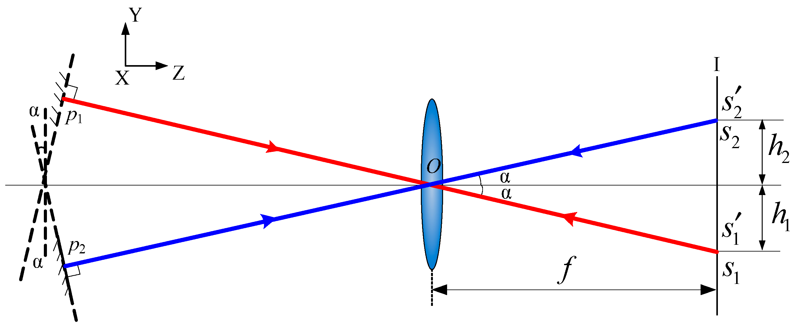
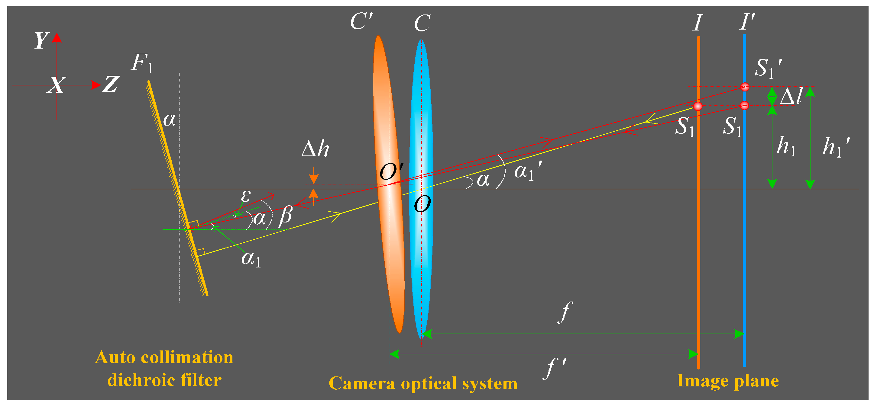
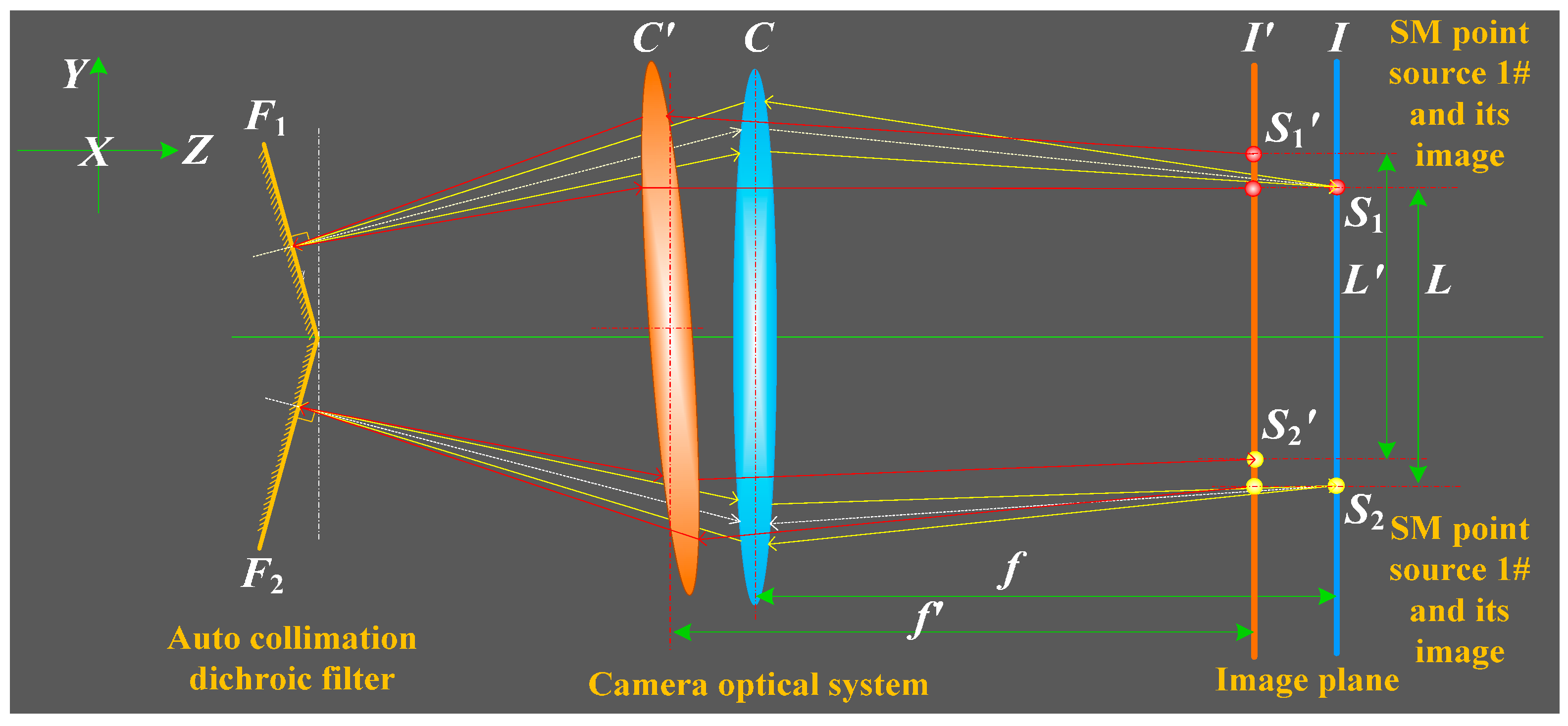
3. Calibration Calculation Based on Differential SMFPs

We adopt two SMFPs to build a differential structure for calculating calibration. Two conjugate SMFPs are symmetrically installed on the focal planes of optical system of the camera. In the red SMFP, lights emitted by point sources pass through beam splitters and into the optical system of the camera. Lights from the primary mirror become collimated light because the SMFP is located on the focal plane of the camera. The collimated lights are reflected by one of the dichroic filter planes into the primary mirror and through the other mirrors of the camera system. Thereafter, lights from the focusing mirror pass through the source prism and approach the CMOS of the red SMFP. The principle of the blue SMFP is the same with that of the red focal plane.

We consider an ideal optical system. The imaging relationship of the equivalent optical paths of self-calibration in an ideal optical system is shown in Figure 6. The auto-collimating light path of S₁ is composed of an SM point source S₁, a camera optical system, an auto-collimation dichroic filter, and an image detector. We use OXYZ to represent the camera coordinate system. In the OXYZ, the origin is the center of the optical system of the remote sensing camera. The origin of the coordinate system could be taken as a point O(0 0 0)^T. We define z-axis as the optical axis, and its positive direction is from left to right; y-axis is perpendicular to the z-axis, and its positive direction is from the bottom going up; x-axis is perpendicular to the paper surface, and its positive direction is vertically shooting out from the paper. The image plane is denoted by I and locates f units along optic axis, where f is the focal length of optical system. The SM point sources S₁ and S₂ and receiver are located on the focal plane of optical camera I. The position vectors of two point sources S₁ and S₂ are defined as ${\stackrel{\rightharpoonup }{S}}_1{(\begin{array}{ccc}0& -h_1& f\end{array})}^T$ and ${\stackrel{\rightharpoonup }{S}}_2{(\begin{array}{ccc}0& h_2& f\end{array})}^T$, where h₁ and h₂ are the distances between the SM point sources S₁ and S₂ and optical axis, respectively. The distance between the SM point source S₂ and optical axis is h₂. The normal vectors of the direction vector of dichroic filter are defined as ${\stackrel{\rightharpoonup }{n}}_1{(\begin{array}{ccc}0& -\sin \alpha & \cos \alpha \end{array})}^T$ and ${\stackrel{\rightharpoonup }{n}}_2{(\begin{array}{ccc}0& \sin \alpha & \cos \alpha \end{array})}^T$, where α is the rotated angle of dichroic filter around the x-axis; that is, the angle between dichroic filter and y-axis. The direction vector of two point sources S₁ and S₂ are defined as ${\stackrel{\rightharpoonup }{l}}_1{(\begin{array}{ccc}0& \sin \alpha & -\cos \alpha \end{array})}^T$ and ${\stackrel{\rightharpoonup }{l}}_2{(\begin{array}{ccc}0& -\sin \alpha & -\cos \alpha \end{array})}^T$.

According to the optical path of camera, the prime light ray emitted from point source S₁ is auto-collimating light when it passes through the camera lenses. Images of the two conjugate point sources are located on S₁′ and S₂′. The auto-collimating lights are reflected by the auto-collimation dichroic filter first and then return into the camera lens. Outgoing lights from the camera are incidents on the focal plane detector. Given that the angle between the prime light ray and optical axis is the same as the normal of dichroic filter, the optical path is auto-collimated; therefore, the position of SM point source and its image coincides. The intersection points of the incoming rays with the dichroic filter are:

$${\stackrel{\rightharpoonup }{p}}_1={\stackrel{\rightharpoonup }{S}}_1+t_1\cdot {\stackrel{\rightharpoonup }{l}}_1,t_1=-\frac{\left({\stackrel{\rightharpoonup }{n}}_1,\stackrel{\rightharpoonup }{O}-{\stackrel{\rightharpoonup }{S}}_1\right)}{\left({\stackrel{\rightharpoonup }{n}}_1,{\stackrel{\rightharpoonup }{l}}_1\right)}$$

(2)

$${\stackrel{\rightharpoonup }{p}}_2={\stackrel{\rightharpoonup }{S}}_2+t_2\cdot {\stackrel{\rightharpoonup }{l}}_2,t_2=-\frac{\left({\stackrel{\rightharpoonup }{n}}_2,\stackrel{\rightharpoonup }{O}-{\stackrel{\rightharpoonup }{S}}_2\right)}{\left({\stackrel{\rightharpoonup }{n}}_2,{\stackrel{\rightharpoonup }{l}}_2\right)}$$

(3)

where $(\cdot ,\cdot )$ denotes the vector scalar products. The direction $\stackrel{\rightharpoonup }{l_1^{\prime }}$ and ${\stackrel{\rightharpoonup }{l}}_1$ of the reflected ray is:

$$\stackrel{\rightharpoonup }{l_1^{\prime }}={\stackrel{\rightharpoonup }{l}}_1-2({\stackrel{\rightharpoonup }{n}}_1,{\stackrel{\rightharpoonup }{l}}_1)\cdot {\stackrel{\rightharpoonup }{n}}_1$$

(4)

$$\stackrel{\rightharpoonup }{l_2^{\prime }}={\stackrel{\rightharpoonup }{l}}_2-2({\stackrel{\rightharpoonup }{n}}_2,{\stackrel{\rightharpoonup }{l}}_2)\cdot {\stackrel{\rightharpoonup }{n}}_2$$

(5)

Finally, we obtain the equation of the outgoing ray

$${\stackrel{\rightharpoonup }{S}}_1^{\prime }(k_1)={\stackrel{\rightharpoonup }{p}}_1+k_1\cdot \stackrel{\rightharpoonup }{l_1^{\prime }}$$

(6)

$${\stackrel{\rightharpoonup }{S}}_2^{\prime }(k_2)={\stackrel{\rightharpoonup }{p}}_2+k_2\cdot \stackrel{\rightharpoonup }{l_2^{\prime }}$$

(7)

where k₁ and k₂ are the system parameters. Intersecting the ray with the image plane parallel to the XOY plane at the distance f from the origin and rewriting Equations (6) and (7) explicitly we get

$$\left[\begin{array}{c}{S}_{1x}^{\prime }\\ S_{1y}^{\prime }\\ S_{1z}^{\prime }\end{array}\right]=\left[\begin{array}{c}{p}_{1x}+\frac{f-p_{1z}}{l_{1z}^{\prime }}\cdot l_{1x}^{\prime }\\ p_{1y}+\frac{f-p_{1z}}{l_{1z}^{\prime }}\cdot l_{1y}^{\prime }\\ f\end{array}\right]$$

(8)

$$\left[\begin{array}{c}{S}_{2x}^{\prime }\\ S_{2y}^{\prime }\\ S_{2z}^{\prime }\end{array}\right]=\left[\begin{array}{c}{p}_{2x}+\frac{f-p_{2z}}{l_{2z}^{\prime }}\cdot l_{2x}^{\prime }\\ p_{2y}+\frac{f-p_{1z}}{l_{2z}^{\prime }}\cdot l_{2y}^{\prime }\\ f\end{array}\right]$$

(9)

According to Equations (8) and (9), the equation of the optical path is as follows:

$${\stackrel{\rightharpoonup }{S}}_i={\left[\begin{array}{ccc}0& {(-1)}^i{h}_i& f\end{array}\right]}^T=\left[\begin{array}{ccc}0& {(-1)}^{i}f\tan \alpha & f\end{array}\right]$$

(10)

where ${\stackrel{\rightharpoonup }{S}}_i$ is the position vector of point source $S_i$, I = 1 or 2. In an ideal optical system, the principal distance is its focal length. Let their respective images $S_1^{\prime }$ and $S_2^{\prime }$ in the focal plane coordinate system be located at $\left(x_{S_1^{\prime }},y_{S_1^{\prime }}\right)$ and $\left(x_{S_2^{\prime }},y_{S_2^{\prime }}\right)$. The principal point can then be expressed as:

$$u_y=\frac{y_{S_1^{\prime }}+y_{S_2^{\prime }}}{2},u_x=\frac{x_{S_1^{\prime }}+x_{S_2^{\prime }}}{2}$$

(11)

When the optical system of a camera exhibits maladjustments, its prime planar position, principal point, and principal distance change accordingly. Considering the influences of different maladjustments of optical components on the first-order parameters of optical cameras, the change in the axial maladjustments of an optical component can vary the primary plane position and principal distance. Moreover, the deviation of an optical component from its original position in a vertical direction can vary the primary plane position, principal point, and principal distance. Furthermore, the slant of an optical component from its original position in a vertical direction can vary the primary plane position, principal point, and principal distance. During on-orbit imaging, a space camera estimates image quality and determines the adjustment operation of the focal length. Focusing can change the installed planes of the SM point sources and image sensor. The optical path when optical system of a camera presents maladjustments during focusing is shown in Figure 7.

In Figure 7, yellow lines represent the original auto-collimating lights while red lines represent the auto-collimating lights of optical system with maladjustments. In the auto-collimating light path, the SMFPs are located on position I of optical system C without maladjustments. The lights emitted from the SM point sources S₁ and S₂ on the symmetrical SMFPs pass through the camera lens and dichroic filters F₁ and F₂, and these lights return to the positions of S₁′ and S₂′. The positions of S₁′ and S₂′ are coincidental with those of S₁ and S₂, respectively. The relative position vector of the image points of two SMFPs is defined as $\stackrel{\rightharpoonup }{L}{(\begin{array}{ccc}0& L& 0\end{array})}^T$. When the optical camera is maladjusted, the SMFP is located on position I′ after focusing. In Figure 7, C′ represents the maladjusted optical system. The lights emitted from the symmetrical SM point sources S₁ and S₂ on I′ pass through the camera lens and dichroic filter, and these lights return to the positions of S₁′ and S₂′ on I′. The relative position vector of the image points of two SMFPs is defined as ${\stackrel{\rightharpoonup }{L}}^{\prime }{(\begin{array}{ccc}0& L^{\prime }& 0\end{array})}^T$. Considering that the auto-collimating light paths of S₁ and S₂ present the same spread rules, we first analyze the lights emitted from S₁. The imaging relationship of S₁ is shown in Figure 8.

In Figure 8, yellow lines are original auto-collimating light paths. Red lines are optical paths of the maladjusted optical system. I′ is the focal plane of the maladjusted optical system. When the focal plane is located on position I for the optical system without maladjustments, the direction vector of outgoing light ray from S₁ is ${\stackrel{\rightharpoonup }{d}}_1{(\begin{array}{ccc}0& -\sin \alpha & -\cos \alpha \end{array})}^T$. The origin of the system C could be taken as a point O(0 0 0)^T. The position vector of the image point of S1 for the optical system without maladjustments ${\overrightarrow{S}}_{d1}$ is:

$${\overrightarrow{S}}_{d1}=\left[\begin{array}{ccc}{O}_x+\frac{f-O_z}{d_{1z}}{d}_{1x}& O_y+\frac{f-O_z}{d_{1z}}{d}_{1y}& f\end{array}\right]$$

(12)

When the focal plane is located on position I′ for the optical system with maladjustments, the direction vector of outgoing light ray from S1 is ${\stackrel{\rightharpoonup }{d}}_1^{\prime }{(\begin{array}{ccc}0& -\sin {\alpha }_1& -\cos {\alpha }_1\end{array})}^T$. The position vector ${\stackrel{\rightharpoonup }{h}}_1{\left[\begin{array}{ccc}0& h_1& f\end{array}\right]}^T$ of point source S1 can be calculated by Equation (10). For the optical system with maladjustments, the deviation vector between the principal point and its original optical axis is $\Delta \stackrel{\rightharpoonup }{h}{\left[\begin{array}{ccc}0& \Delta h& 0\end{array}\right]}^T$. In Figure 8, the origin of the system C′ could be taken as a point O’(0 Δh 0)T. For optical system with long focal length, the distance ∆h is small and can be neglected. The relationship between point source S1 and direction vector ${\stackrel{\rightharpoonup }{d}}_1^{\prime }$ can be expressed as

$${\stackrel{\rightharpoonup }{h}}_1=\Delta \stackrel{\rightharpoonup }{h}+{\left[\begin{array}{ccc}0& f^{\prime }\frac{d_{1y}^{\prime }}{d_{1z}^{\prime }}& f^{\prime }\end{array}\right]}^T\approx {\left[\begin{array}{ccc}0& f^{\prime }\frac{d_{1y}^{\prime }}{d_{1z}^{\prime }}& f^{\prime }\end{array}\right]}^T$$

(13)

The normal vector of the direction vector of dichroic filter is ${\stackrel{\rightharpoonup }{n}}_{F_1}{(\begin{array}{ccc}0& \sin \alpha & \cos \alpha \end{array})}^T$. The direction vector of the incoming rays on dichroic filter is $\stackrel{\rightharpoonup }{e}{(\begin{array}{ccc}0& -\sin {\alpha }_1& -\cos {\alpha }_1\end{array})}^T$. The angle of incidence between the incidence lights and dichroic filter plane is ε = α − α1. The angle between outgoing rays and z-axis is β = ε + α = 2α − α1. The direction vector of the outgoing rays from dichroic filter is

$$\stackrel{\rightharpoonup }{b}=\stackrel{\rightharpoonup }{e}-2({\stackrel{\rightharpoonup }{n}}_{F_1},\stackrel{\rightharpoonup }{e})\cdot {\stackrel{\rightharpoonup }{n}}_{F_1}$$

(14)

Given that plane I′ is the focal plane of the current maladjusted focal plane, the lights emitted from point source S₁ are parallel when they pass through the camera system. Therefore, one of the rays reflected by the dichroic filter element passes through the center of the prime plane first and then return into S₁′. The direction vector of the outgoing rays from prime plane F₁ is ${\stackrel{\rightharpoonup }{c}}_1{(\begin{array}{ccc}0& \sin {{\alpha }^{\prime }}_1& \cos {{\alpha }^{\prime }}_1\end{array})}^T$. The position vector of S₁′ is ${\stackrel{\rightharpoonup }{S}}_1^{\prime }{(\begin{array}{ccc}0& {h^{\prime }}_1& f^{\prime }\end{array})}^T$. The following relationship can be satisfied as

$$\{\begin{array}{l}\stackrel{\rightharpoonup }{b}={\stackrel{\rightharpoonup }{c}}_1\\ {\stackrel{\rightharpoonup }{S}}_1^{\prime }={\left[\begin{array}{ccc}{O}_x^{\prime }+\frac{f^{\prime }-O_z^{\prime }}{c_{1z}}{c}_{1x}& O_y^{\prime }+\frac{f^{\prime }-O_z^{\prime }}{c_{1z}}{c}_{1y}& f^{\prime }\end{array}\right]}^T\end{array}$$

(15)

Using the same method, the above imaging relationship of point source S₂ can be obtained. The variation vector of relative position of image points of two SMFPs can be expressed as

$$\begin{array}{l}\Delta \stackrel{\rightharpoonup }{l}={\left[\begin{array}{ccc}0& \Delta l& 0\end{array}\right]}^T={\stackrel{\rightharpoonup }{L}}^{\prime }-\stackrel{\rightharpoonup }{L}={\stackrel{\rightharpoonup }{S}}_1^{\prime }-{\stackrel{\rightharpoonup }{S}}_1^{\prime }-\left({\overrightarrow{S}}_{d1}-{\overrightarrow{S}}_{d2}\right)\\ O_y^{\prime }+\frac{f^{\prime }-O_z^{\prime }}{c_{1z}}{c}_{1y}-\left(O_y^{\prime }+\frac{f^{\prime }-O_z^{\prime }}{c_{2z}}{c}_{2y}\right)\\ -\left(O_y+\frac{f-O_z}{d_{1z}}{d}_{1y}-\left(O_y+\frac{f^{\prime }-O_z^{\prime }}{d_{2z}}{d}_{2y}\right)\right)\end{array}$$

(16)

where ${\stackrel{\rightharpoonup }{c}}_2{(\begin{array}{ccc}0& \sin {\alpha }_2^{\prime }& \cos {\alpha }_2^{\prime }\end{array})}^T$, which is the direction vector of the outgoing rays from primary plane F₂, ${\stackrel{\rightharpoonup }{d}}_2{(\begin{array}{ccc}0& \sin \alpha & -\cos \alpha \end{array})}^T$ is the direction vector of outgoing light ray from S₂ when the focal plane is located on position I for the optical system without maladjustments. Substituting Equations (13)–(15) into Equation (16), a new equation is obtained as:

$$2\times \tan \left(2\alpha \right)\times {f^{\prime }}^2-(4h_i+\Delta l)\times f^{\prime }-(2h_i+\Delta l)\times h_i\times \tan \left(2\alpha \right)=0$$

(17)

Solving the above equation, the mathematical model of principal distance can be expressed as:

$$f^{\prime }=\frac{4h_i+\Delta l+{\left[{(4h_i+\Delta l)}^2+8h_i\times (4h_i+\Delta l){\left(\tan 2\alpha \right)}^2\right]}^{\frac{1}{2}}}{4\tan 2\alpha }$$

(18)

where $\alpha$ and $h_i$ are the designed values. Using the same principle, the principal point can be expressed as:

$$u_{x/y}=\frac{x_{s_1^{\prime }}+x_{s_2^{\prime }}-\Delta l-2h_i}{2}$$

(19)

The variation $\Delta l$ is the distance in the centroid of point images of SMFP. The point images are captured by two CMOS sensors on SMFP. The centroid extraction algorithm is used to calculate the centroid of point images. On the basis of variation $\Delta l$, principal distance and principal point can be calculated by Equations (18) and (19).

4. Experiment and Analysis

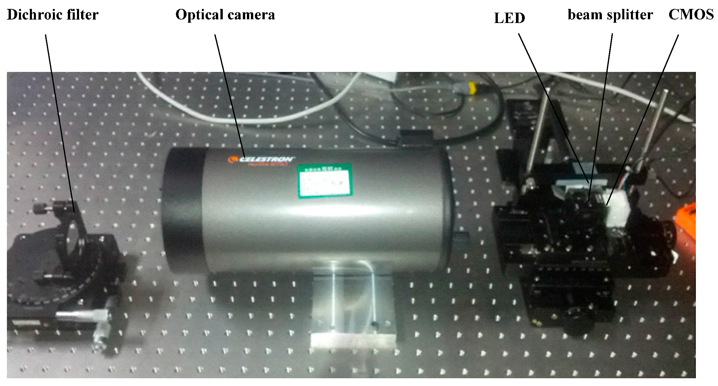
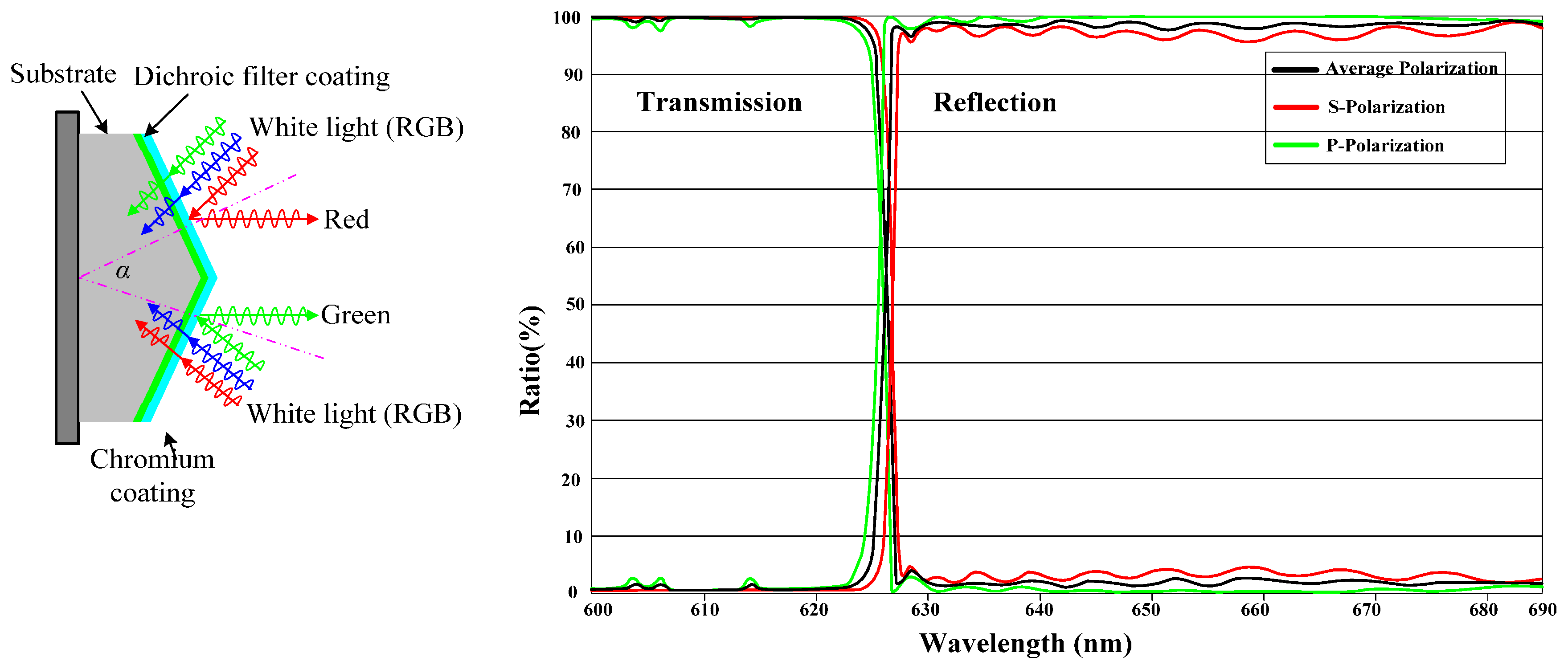
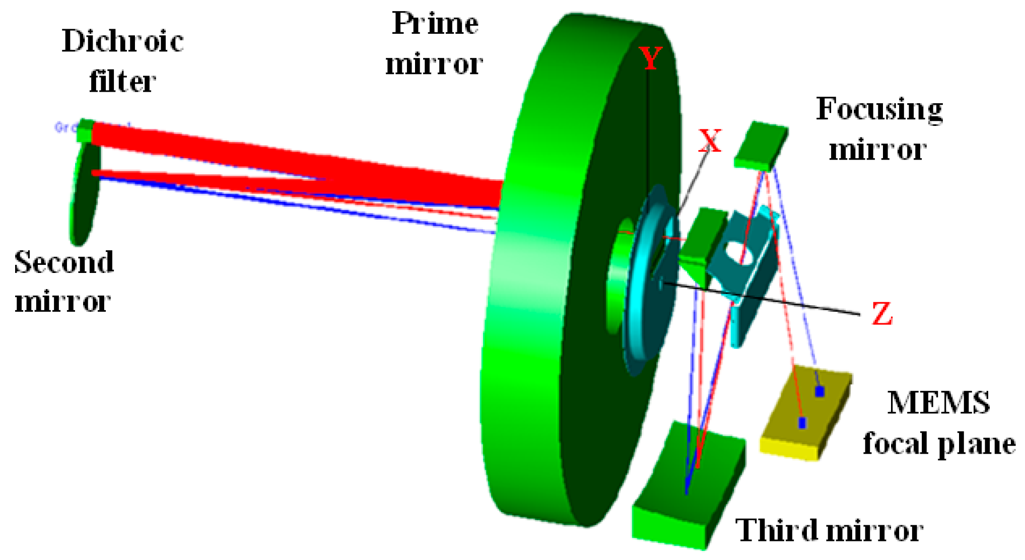
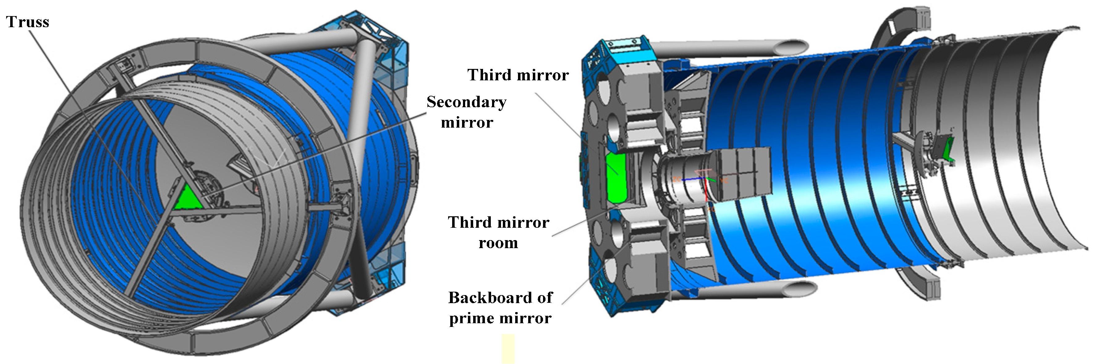
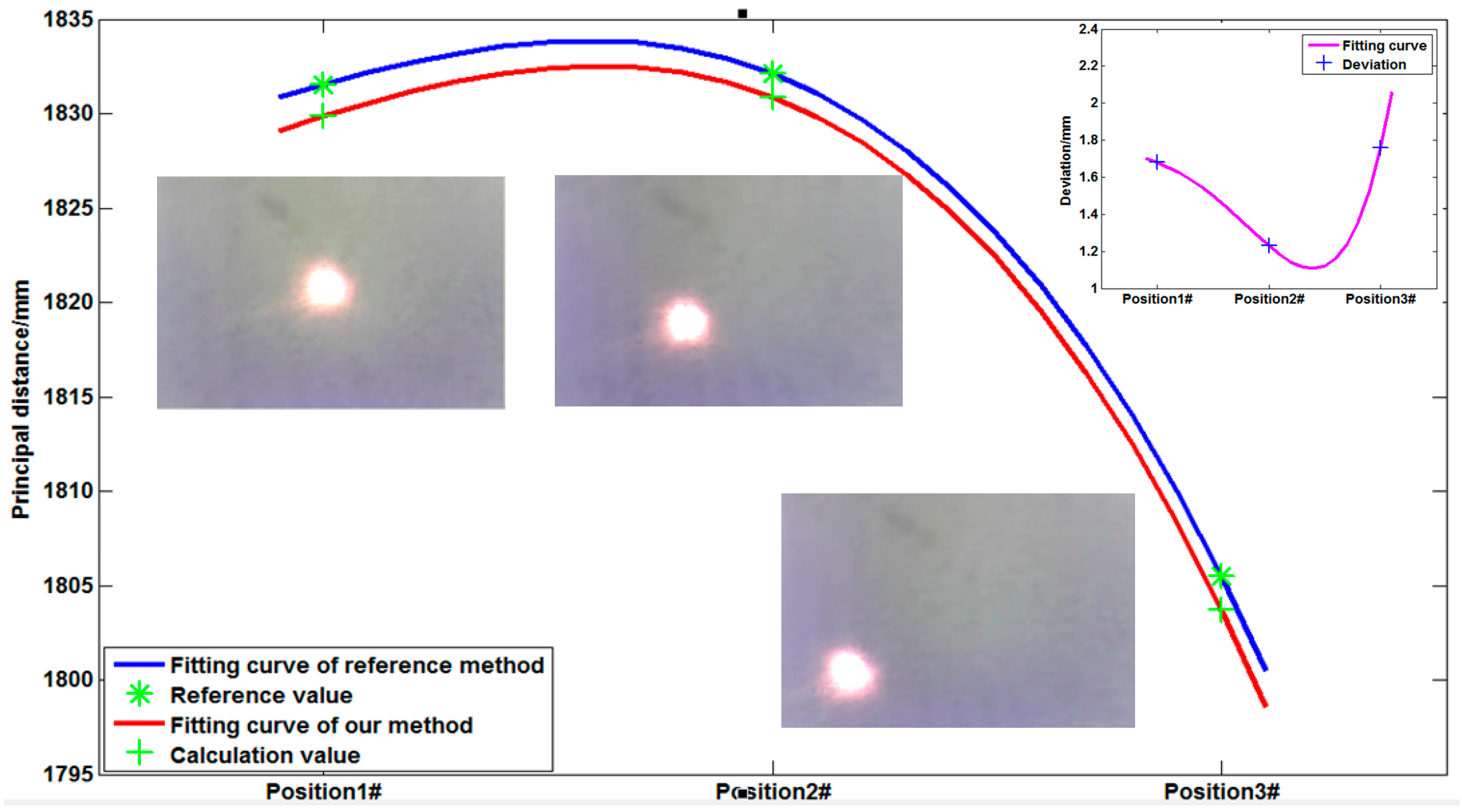
4.1. Experiment of Optical System

To verify the effectiveness of the proposed method, we use ZEMAX in simulating the calibration experiments. ZEMAX presents high accuracy of ray tracing. For a maladjusted optical system, the coordinate positions from rays with different fields of view (FOV) positions to the image plane can be traced accurately. In each experiment, the reference values of principal distance and principal point are first calculated. We use the on-ground calibration method based on measuring angles to calibrate the reference values of principal distance and principal point. The laboratory measuring angle method is widely used in calibrating IOPs of remote sensing cameras [20,21,22,23,24,25]. In this method, an uncalibrated optical camera is placed on a precision turntable to capture the parallel lights of star points emitted by a collimator. At different rotation angles of the turntable, the camera can obtain multiple positions of star points and their images from different FOV positions. The recorded rotation angle and image point positions are used to build an imaginary geometrical equation between each star point and its image. According to the principle of camera distortion, an optical camera has its minimum distortion at its principal point location. A least squares method is used to solve the imaging geometrical equation for calculating principal distance and principal point. This method is simple and can achieve a micrometer-level calibration accuracy. Similar to the ground calibration method of principal distance and principal point, we use the least squares and multiple regression analyses to calculate the principal distance and principal point of each test and maladjusted system. Principal distance and principal point can be expressed as follows:

$$f=\frac{\left({\displaystyle \sum _{i=1}^N{L}_i{\tan }^2{W}_i\cdot {\displaystyle \sum _{i=1}^N{\tan }^3{W}_i}}\right)-\left({\displaystyle \sum _{i=1}^N{L}_i\tan W_i\cdot {\displaystyle \sum _{i=1}^N{\tan }^4{W}_i}}\right)}{{\left({\displaystyle \sum _{i=1}^N{\tan }^3{W}_i}\right)}^2-\left({\displaystyle \sum _{i=1}^N{\tan }^2{W}_i\cdot {\displaystyle \sum _{i=1}^N{\tan }^4{W}_i}}\right)}$$

(20)

$$p_{x/y}=\frac{\left({\displaystyle \sum _{i=1}^N{L}_i{\tan }^2{W}_i\cdot {\displaystyle \sum _{i=1}^N{\tan }^2{W}_i}}\right)-\left({\displaystyle \sum _{i=1}^N{L}_i\tan W_i\cdot {\displaystyle \sum _{i=1}^N{\tan }^3{W}_i}}\right)}{{\left({\displaystyle \sum _{i=1}^N{\tan }^3{W}_i}\right)}^2-\left({\displaystyle \sum _{i=1}^N{\tan }^2{W}_i\cdot {\displaystyle \sum _{i=1}^N{\tan }^4{W}_i}}\right)}$$

(21)

where $f$ is the principal distance, $p_{x/y}$ is the position of the principal point in the x direction or the y direction, i is the number of measurement points, $W_i$ is the measurement angle of the ith measurement point, and $L_i$ is the measurement height of the ith measurement point.

In the first step of experimentation, we use an ideal optical system to perform modeling because the ideal optical system does not exhibit aberrations and can adequately verify our method. In ZEMAX, the focal length and aperture diameter of our input optical system model are 4500 and 600 mm, respectively. Moreover, a mirror with a deflecting angle of 0.7° is used to simulate the dichroic filter. The ideal optical path is shown in Figure 9. We set different maladjustments for S₂ and use two different methods to calculate the principal distance of different maladjusted optical systems. In our simulation, we use 10 reference points at different FOV positions to estimate principal distances and principal points for the on-ground method.

We set several maladjustments of S₂ along the z direction to test the proposed method. The deviations of the S₂ mirror from its original position are from 0.010 mm to 0.05 mm. Then, we set maladjustments along the y direction and around the x- and y-axes. Along the y direction, we set two maladjustments of S₂ to test the proposed method. The deviations of the S₂ mirror from its original position are 0.020 mm along the x and y directions. Thereafter, we set several maladjustments of S₂ around the x-axis to test the proposed method. The deviations of the S₂ mirror from its original position are 30 s of arc around the x- and y-axes. The calculated results of the principal distance in the simulated conditions with different maladjustments of optical system are shown in

Table 1. Simulation calculation results using ground method.

Maladjustments	f (mm)	Δf (mm)
Z direction + 0.01	4498.594192	−1.405808
Z direction + 0.015	4497.891609	−2.108391
Z direction + 0.02	4497.189260	−2.810740
Z direction + 0.05	4492.979717	−7.020283
Slant 30′′ around X	4499.999777	−0.000223
Slant 30′′ around Y	4499.999780	−0.000220
Decentration 0.02 mm in X direction	4499.999997	−2.68 × 10−6
Decentration 0.02 mm in Y direction	4499.999999	−1.32 × 10−6

and

Table 2. Simulation calculation results of the proposed method.

Maladjustments	Δl (mm)	Δf (mm)	Deviation (μm)
Z direction + 0.01	−0.068704	−1.405803	4.82 × 10−3
Z direction + 0.015	−0.103040	−2.108378	1.27 × 10−2
Z direction + 0.02	−0.137366	−2.810749	−9.24 × 10−3
Z direction + 0.05	−0.343092	−7.020266	1.71 × 10−2
Slant 30′′ around X	−0.000010	−0.000203	1.95 × 10−2
Slant 30′′ around X	−0.000010	−0.000203	1.75 × 10−2
Decentration 0.02 mm in X direction	0	0	2.68 × 10−3
Decentration 0.02 mm in Y direction	0	0	1.32 × 10−3

. In Table 2, Δl is the variation of relative positions of the two SMFPs (Equation (16)). Compared with the error in the on-ground method, the error in our method is less than 0.02 µm. The error is attributed to the round-off error, ignoring ∆h, and focusing.

In the second step, we use an actual optical system in performing the modeling. The actual optical system presents aberration and is thus used to further verify our method. Our input optical system model parameters areas follows: the focal length is 8000 mm, the aperture diameter is 600 mm, the relative aperture is 1/13.3, FOV is 1.8°, and deflected FOV is 0.578°. Moreover, the co-axial, three-mirror-anastigmatic optical system with deflected FOV is adopted. The optical system is composed of three aspherical and two spherical mirrors. These mirrors build an optical path of the secondary imagery. On the first image plane, a folding mirror is placed and rotated along the light direction by 90°. Based on this optical system, we design a calibrated optical path. The dichroic filter that provides angle information is installed on the truss of the secondary mirror. Based on the size of the truss and the absence of extra obstruction, the size of the dichroic filter is designed to 40 mm × 40 mm under the condition of no additional blocking incident rays. The FOV and deflected angle of dichroic filter are designed based on the space camera. he parameters of the dichroic filter component are shown

Table 3. Parameters of the dichroic filter component.

Parameters	Value
Size	40 mm × 40 mm
Coordinate in the X direction	±97.743
Corresponding FOV in the X direction	±0.7°
Coordinate in the Y direction	−76.797
Corresponding FOV in the Y direction	−0.55°

. The calibrated optical path designed based on the auto-collimating method and designed parameters is shown in Figure 10. The optical rays are reflected from the mirror, passes through the optical system twice, and then concentrates on the CMOS detector.

The optical system is composed of primary, secondary, tertiary, folding, and focusing mirrors. The maladjustments of the system can be attributed to axial maladjustment, vertical axis decentration, and slanting. By analyzing the maladjustments of the different elements of the optical system, we determine that the secondary and tertiary mirror maladjustments significantly affect the focal plane of the optical system. Given that the tertiary mirror is installed in the third mirror room, nearly no maladjustment occurs in the mirror. The highest effect is from the secondary mirror because it is installed on the truss of the camera (Figure 11). In actual on-orbit work, the truss of camera is easily changed by platform vibration. Therefore, the largest effect on the IOPs of the camera comes from the secondary mirror. Moreover, we set different maladjustments for the secondary mirror. Using the same approach, we set 10 reference points in a valid FOV and set maladjustments along the z direction. Furthermore, we set several maladjustments of S₂ along the z direction to test the proposed method. The deviations of the S₂ mirror from its original position are from 0.002 mm to −0.02 mm. We set maladjustments along the y direction and around the x- and y-axes. Along the y direction, we set two maladjustments of S₂ to test the proposed method. The deviations of the S₂ mirror from its original position are both 0.020 mm along the x and y directions. We set several maladjustments of S₂ around the x-axis to test the proposed method. The deviations of the S₂ mirror from its original position are both 5s of arc around the x- and y-axes. The calculated results of the principal distance in the simulation conditions with different maladjustments of optical system are shown in

Table 4. Simulation calculation results using ground method.

Maladjustments	f (mm)
Z direction + 0.002	8001.8321
Z direction + 0.005	8006.0262
Z direction + 0.01	8013.0772
Z direction + 0.015	8020.0584
Z direction + 0.02	8027.0893
Slant 5′′ around X	7998.8212
Slant 5′′ around Y	7999.0352
Decentration 0.02 mm in X direction	7999.0317
Decentration 0.02 mm in Y direction	7999.1658

and

Table 5. Simulation calculation results using the proposed method.

Maladjustments	Δl (mm)	Δf (mm)	Deviation (mm)
Z direction + 0.002	0.1030	8001.8326	0.0005
Z direction + 0.005	0.3080	8006.0273	0.0011
Z direction + 0.01	0.6524	8013.0742	−0.003
Z direction + 0.015	0.9936	8020.0557	−0.003
Z direction + 0.02	1.3372	8027.0865	−0.003
Slant 5′′ around X	−0.0448	7998.8083	−0.013
Slant 5′′ around Y	−0.0336	7999.0374	0.0022
Decentration 0.02 mm in X direction	−0.0338	7999.0333	0.0017
Decentration 0.02 mm in Y direction	−0.0266	7999.1807	0.0148

. Compared with that in the on-ground method, the error in our method is less than 0.0148 mm.

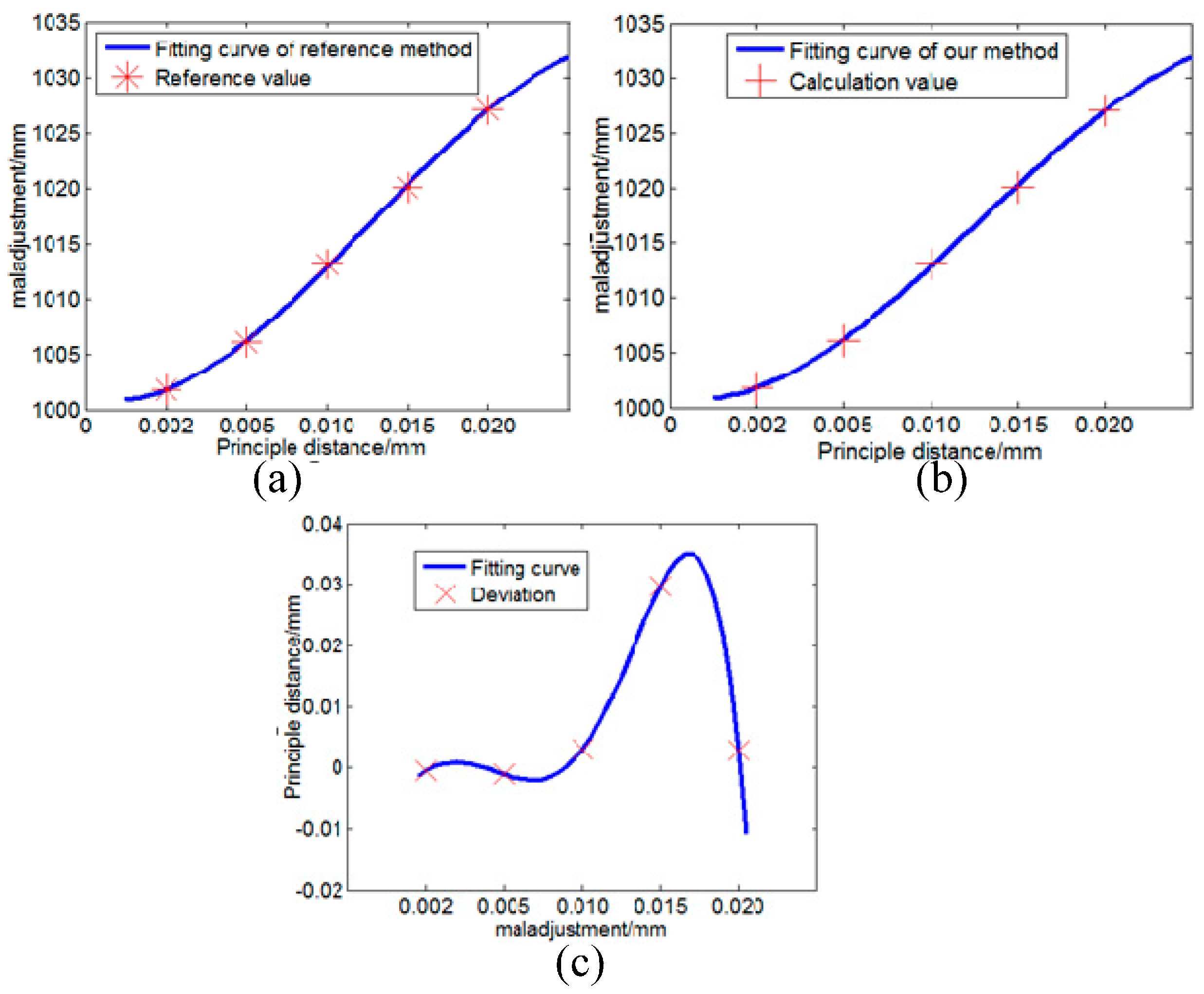
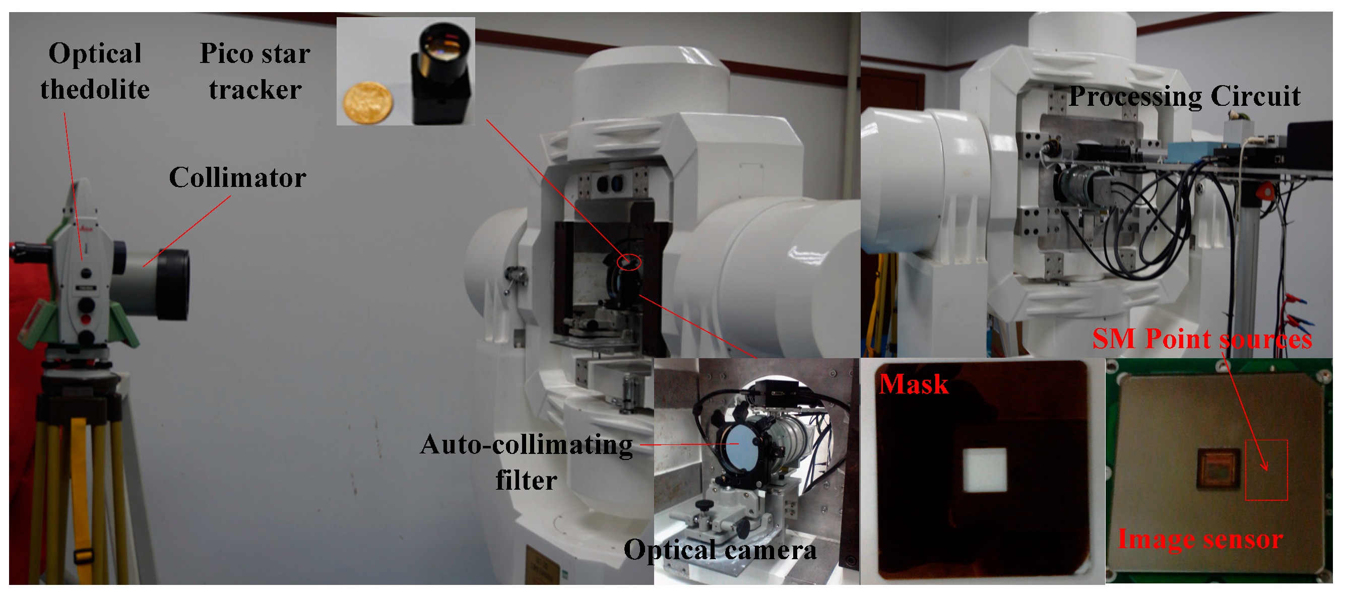
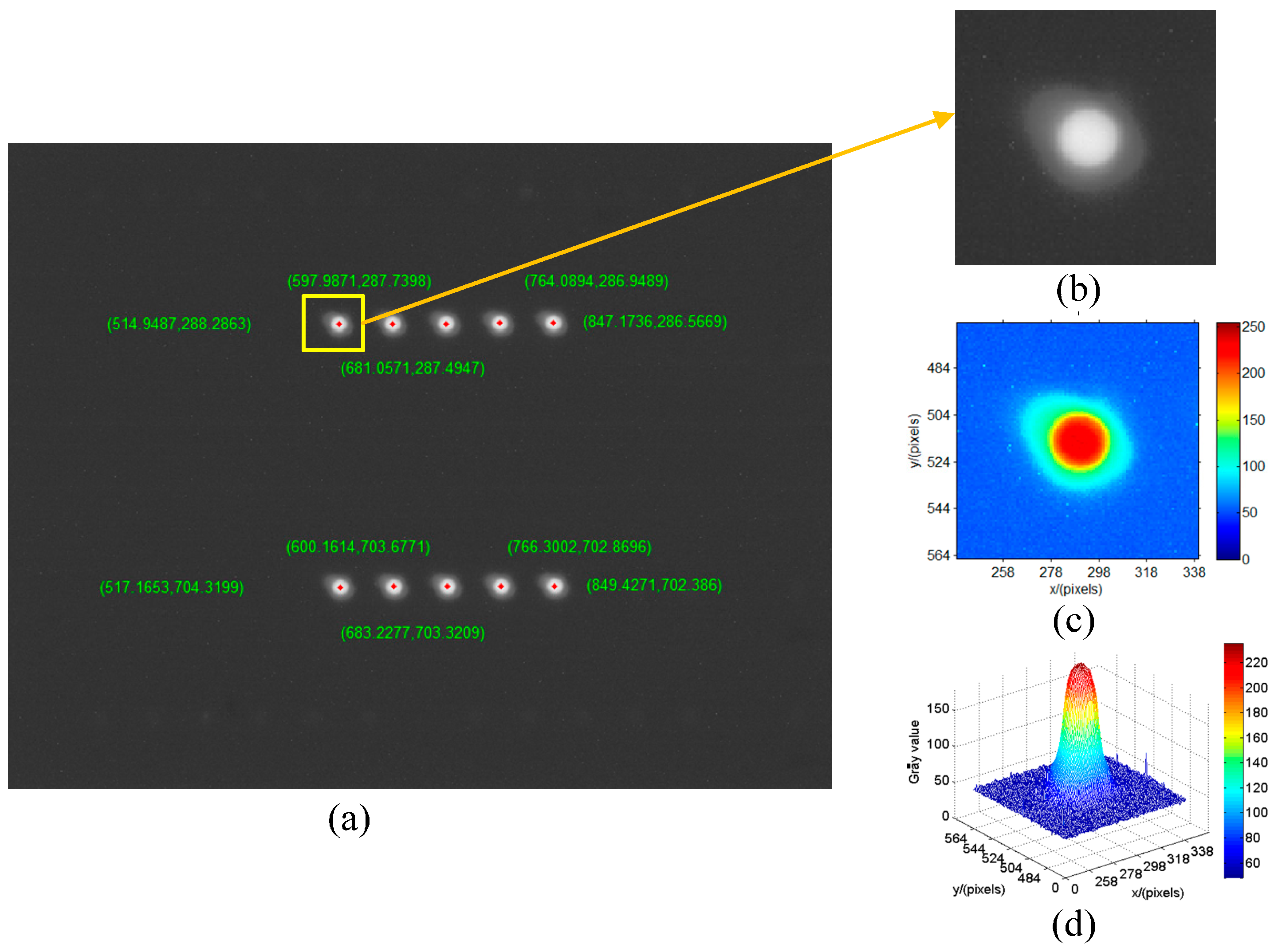
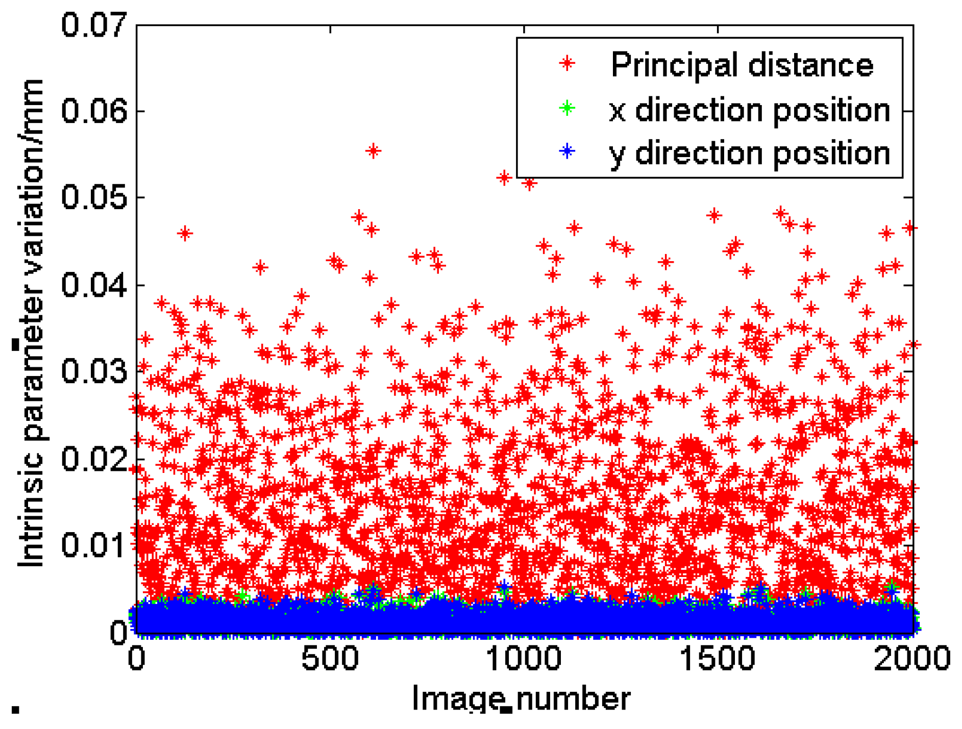
4.2. Experiment of Setup in Lab

In the first step of experimentation, we discretely set up the experimental system components to verify the proposed method. Figure 12 shows the experimental calibration system. The system includes an optical camera, a reflective mirror, horizontal rotation adjustment, 2D displacement platform, an LED, and a CMOS. The F/ratio of the optical system is 11.8 and the aperture diameter is 127 mm.

To verify the proposed method, we use the focusing knob to set three specific positions. We use a known line-pair method to calibrate the principal distance at three positions as reference values. We then perform our method along the three specific positions. Figure 13 shows the captured images and calibrated results at the three positions. The centroids of the three positions are (310.76, 251.12), (242.43, 320.70), and (124.76, 378.99). Compared with the error in the on-ground method, the error in our method is less than 2 mm. The calibration error is large and mainly due to that the tooling fixtures do not achieve the requirements. Therefore, we use the SM method to further improve calibration accuracy.

In the second step, we use SMFP to set up an experimental system for the integrated calibration with imaging to verify the proposed method. Figure 14 shows the experimental calibration system. The system includes an optical camera, an auto-collimating filter, a processing circuit, a collimator, an optical theodolite, and a high-accuracy turntable. The optical system is a co-axial Schmidt–Cassegrain optical system. The aperture diameter is 202.6 mm, the focal length is 1026 mm, and the F/ratio of the optical system is 10. The image sensor is a CMOS detector, and the image resolution is 1280 pixels × 1024 pixels. The SM point sources, beam splitter, and image sensor are installed on the focal plane. A collimator provided an infinite target for the test system. To calibrate the reference value, the three-axis turntable and collimator are adjusted evenly using a level. By adjusting the support tooling of the camera and using the benchmark prisms of the optical axis of camera, the visual axis of camera and collimator are moved to share a common shaft. The camera controller sets the imaging mode. Star points of the collimator are imaged on the target CMOS sensor. The turntable is revolved, and the rotation angle and capture image are recorded. The processing circuit output stars coordinates in real time. Based on the measured centroid position and rotation angle, the least squares and two-multiplication regression analyses are used to obtain the optimal estimation values of the IOPs.

For our method, the camera controller sets the calibration mode and switches the SM point sources on or off. The SM point sources are lighted when the camera controller performs the turn-on command. Figure 15 shows the captured images when the two point sources are lighted. SM optical sources are an ideal point source and can be used in measuring internal parameters. Using the spot centroid algorithm, the position of images can be determined. Principal distance and principal point are calculated using Equations (18) and (19).

We adjust the motion of the secondary mirror to simulate on-orbit maladjustments of the optical system. From analyzing the maladjustments of the different elements of the optical system, we observe that the secondary and primary mirror maladjustments affect the focal plane of the optical system. Given that the primary mirror is installed in the primary mirror room, it exhibits nearly no maladjustment. Figure 16 shows the principal distance variation under different maladjustments. We use the ground calibration method based on the least squares and multiple regression analyses as reference. The calibration deviation is less than 0.035 mm. The deviation is attributed to the self-method error between methods under the maladjusted condition.

To test the monitoring accuracy of our method with an approximation to the on-orbit environment, our experiment is performed in a laboratory with constant temperature. The experimental turntable uses a gas-floating vibration isolation platform to avoid vibration disturbance. We use our method to monitor the variation in principal distance and principal point in the static case. We process tens of thousands of images to calculate the monitoring accuracy. The variations in principal distance and principal point position in 2000 real-time seconds are shown in Figure 17. Based on the statistical data in Figure 17, the mean square error formula is used to calculate the monitoring accuracy. The monitoring accuracy of the principal distance can reach 0.017 mm. Furthermore, the monitoring accuracy of the principal point can reach 0.005 and 0.0049 mm in the x and y directions, respectively. For example, the camera exhibits a 5 m image positioning accuracy; therefore, the camera requires less than 50 µm calibration accuracy of principal distance and principal point. Moreover, the monitoring accuracy can reach micrometer level and meet the mapping requirements of camera.

5. Conclusions

In this work, we propose the SMPF and BADF methods for constructing an on-orbit calibration method of camera with high accuracy. The BADF and SMPF methods are integrated into a camera. First, the point sources are installed on the focal plane, the SM method is used to fabricate point sources, and these point sources are packaged with the image sensor and beam splitter. Second, we integrate the auto-collimation dichroic filter into the optical system of the camera. Third, a mathematical model of IOPs is built based on a geometrical imaging model. Fourth, the centroid extraction algorithm is used to process images to extract the star point positions and calculate the IOPs. Finally, we use ZEMAX to simulate the proposed method and set up an experiment for verifying the feasibility of our method with micrometer-level monitoring accuracy. The proposed method can complete self-calibration without temporal and spatial limitations in real time. Our method can also be applied to improve the performance of other calibration methods.

References

1. Stuffler, T.; Kaufmann, C.; Hofer, S.; Forster, K.P.; Schreier, G.; Mueller, A.; Eckardt, A.; Bach, H.; Penne, B.; Benz, U. The EnMAP hyperspectral imager—An advanced optical payload for future applications in Earth Observation programmes. Acta Astronaut. 2007, 61, 115–120. [Google Scholar] [CrossRef]
2. Teillet, P.M. A status overview of earth observation calibration/validation for terrestrial applications. Can. J. Remote Sens. 1997, 23, 291–298. [Google Scholar] [CrossRef]
3. Fritz, L.W. Commercial earth observation satellites. Int. Arch. Photogramm. Remote Sens. 1996, 31, 273–282. [Google Scholar]
4. Hu, Q. Input shaping and variable structure control for simultaneous precision positioning and vibration reduction of flexible spacecraft with saturation compensation. J. Sound Vib. 2008, 318, 18–35. [Google Scholar] [CrossRef]
5. Wei, M.; Xing, F.; You, Z. An implementation method based on ERS imaging mode for sun sensor with 1 kHz update rate and 1 precision level. Opt. Express 2013, 21, 32524–32533. [Google Scholar] [CrossRef] [PubMed]
6. Sun, T.; Xing, F.; You, Z.; Wei, M. Motion-blurred star acquisition method of the star tracker under high dynamic conditions. Opt. Express 2013, 21, 20096–20110. [Google Scholar] [CrossRef] [PubMed]
7. Skaloud, J.; Cramer, M.; Schwarz, K.P. Exterior orientation by direct measurement of camera position and attitude. Int. Arch. Photogramm. Remote Sens. 1996, 31, 125–130. [Google Scholar]
8. Fraser, C.S.; Ravanbakhsh, M. Georeferencing from Geoeye-1 imagery: Early indications of metric performance. In Proceedings of the International Society for Photogrammetry and Remote Sensing (ISPRS) Hannover Workshop, Hannover, Germany, 2–5 June 2009.
9. Croft, J. GeoEye & ITT team up for out-of-this-world technology. Imaging Notes Mag. 2008, 23. [Google Scholar]
10. Brian, C. Pleiades 1B and SPOT 6 image quality status after commissioning and 1st year in orbit. In Proceedings of the Joint Agency Commercial Imagery Evaluation (JACIE) Workshop, Louisville, KY, USA, 26–28 March 2014.
11. Gaudin-Delrieu, C.; Lamard, J.L.; Cheroutre, P.; Bailly, B.; Dhuicq, P.; Puig, O. The High resolution optical instruments for the Pleiades earth observation satellites. In Proceedings of the 7th International Conference on Space Optics (ICSO), Toulouse, France, 14–17 October 2008.
12. Luquet, P.; Chikouche, A.; Benbouzid, A.B.; Arnoux, J.J.; Chinal, E.; Massol, C.; Rouchit, P.; Zotti, S.D. NAOMI instrument: A product line of compact & versatile cameras designed for high resolution missions in Earth observation. In Proceedings of the 7th International Conference on Space Optics (ICSO), Toulouse, France, 14–17 October 2008.
13. Li, J.; Xing, F.; You, Z. Space high-accuracy intelligence payload system with integrated attitude and position determination. Instrument 2015, 2, 3–16. [Google Scholar]
14. Weng, J.; Cohen, P.; Herniou, M. Camera calibration with distortion models and accuracy evaluation. IEEE Trans. Pattern Anal. Mach. Intell. 1992, 14, 965–980. [Google Scholar] [CrossRef]
15. Liang, J.; Williams, D.R.; Miller, D.T. Supernormal vision and high-resolution retinal imaging through adaptive optics. J. Opt. Soc. Am. A 1997, 14, 2884–2892. [Google Scholar] [CrossRef]
16. Neil, M.A.A.; Booth, M.J.; Wilson, T. Closed-loop aberration correction by use of a modal Zernike wave-front sensor. Opt. Lett. 2000, 25, 1083–1085. [Google Scholar] [CrossRef] [PubMed]
17. Jeong, T.M.; Menon, M.; Yoon, G. Measurement of wave-front aberration in soft contact lenses by use of a Shack-Hartmann wave-front sensor. Appl. Opt. 2005, 44, 4523–4527. [Google Scholar] [CrossRef] [PubMed]
18. Wang, L.L.; Tsai, W.H. Camera calibration by vanishing lines for 3-D computer vision. IEEE Trans. Pattern Anal. Mach. Intell. 1991, 13, 370–376. [Google Scholar] [CrossRef]
19. Hong, Y.; Ren, G.; Liu, E. Non-iterative method for camera calibration. Opt. Express 2007, 23, 23992–24003. [Google Scholar] [CrossRef] [PubMed]
20. Ricolfe-Viala, C.; Sanchez-Salmeron, A.J.; Valera, A. Calibration of a trinocular system formed with wide angle lens cameras. Opt. Express 2012, 20, 27691–27696. [Google Scholar] [CrossRef] [PubMed]
21. Zhang, Z. Camera calibration with one-dimensional objects. IEEE Trans. Pattern Anal. Mach. Intell. 2004, 26, 892–899. [Google Scholar] [CrossRef] [PubMed]
22. Lin, P.D.; Sung, C.K. Comparing two new camera calibration methods with traditional pinhole calibrations. Opt. Express 2007, 15, 3012–3022. [Google Scholar] [CrossRef] [PubMed]
23. Wei, Z.; Liu, X. Vanishing feature constraints calibration method for binocular vision sensor. Opt. Express 2008, 23, 18897–18914. [Google Scholar] [CrossRef] [PubMed]
24. Bauer, M.; Griebbach, D.; Hermerschmidt, A.; Kruger, S.; Scheele, M.; Schischmanow, A. Geometrical camera calibration with diffractive optical elements. Opt. Express 2008, 16, 20241–20248. [Google Scholar] [CrossRef] [PubMed]
25. Ricolfe-Viala, C.; Sanchez-Salmeron, A. Camera calibration under optimal conditions. Opt. Express 2011, 19, 10769–10775. [Google Scholar] [CrossRef] [PubMed]
26. Fu, R.; Zhang, Y.; Zhang, J. Study on geometric measurement methods for line-array stereo mapping camera. Spacecr. Recovery Remote Sens. 2011, 32, 62–67. [Google Scholar]
27. Hieronymus, J. Comparison of methods for geometric camera calibration. Int. Arch. Photogramm. Remote Sens. Spat. Inf. Sci. 2012, 39, 595–599. [Google Scholar] [CrossRef]
28. Yuan, F.; Qi, W.J.; Fang, A.P. Laboratory geometric calibration of areal digital aerial camera. Proc. SPIE 2013, 8921, 99–103. [Google Scholar] [CrossRef]
29. Chen, T.; Shibasaki, R.; Lin, Z. A rigorous laboratory calibration method for interior orientation of airborne linear push-broom camera. Photogramm. Eng. Remote Sens. 2007, 73, 369–374. [Google Scholar] [CrossRef]
30. Wu, G.; Han, B.; He, X. Calibration of geometric parameters of line array CCD camera based on exact measuring angle in lab. Opt. Precis. Eng. 2007, 15, 1628–1632. [Google Scholar]
31. Yuan, F.; Qi, W.; Fang, A.; Ding, P.; Yu, X. Laboratory geometric calibration of non-metric digital camera. Proc. SPIE 2013, 8921, 99–103. [Google Scholar]
32. Heikkila, J.; Silvén, O. A four-step camera calibration procedure with implicit image correction. In Proceedings of the IEEE Computer Society Conference: Computer Vision and Pattern Recognition, Washington, DC, USA, 17–19 June 1997; pp. 1106–1112.
33. Faig, W. Calibration of close-range photogrammetric systems: Mathematical formulation. Photogramm. Eng. Remote Sens. 1975, 41, 1479–1486. [Google Scholar]
34. Simon, T.; Aymen, A.; Pierre, D. Cross-diffractive optical elements for wide angle geometric camera calibration. Opt. Lett. 2011, 36, 4770–4772. [Google Scholar]
35. Yilmazturk, F. Full-automatic self-calibration of color digital cameras using color targets. Opt. Express 2011, 19, 18164–18174. [Google Scholar] [CrossRef] [PubMed]
36. Maybank, S.J.; Faugeras, O.D. A theory of self-calibration of a moving camera. Int. J. Comput. Vis. 1992, 8, 123–151. [Google Scholar] [CrossRef]
37. Faugeras, O.D.; Luong, Q.T.; Maybank, S.J. Camera self-calibration: Theory and experiments. In Proceedings of the Springer European Conference on Computer Vision, Santa Margherita, Italy, 19–22 May 1992; pp. 321–334.
38. Hartley, R.I. Euclidean reconstruction from uncalibrated views. In Proceedings of the Springer Joint European-US Workshop on Applications of Invariance in Computer Vision, Ponta Delgada, Portugal, 9–14 October 1993; pp. 235–256.
39. Song, D.M. A self-calibration technique for active vision system. IEEE Trans Robot. Autom. 1996, 12, 114–120. [Google Scholar] [CrossRef]
40. Caprile, B.; Torre, V. Using vanishing points for camera calibration. Int. J. Comput. Vis. 1990, 4, 127–139. [Google Scholar] [CrossRef]
41. Gonzalez-Aguilera, D.; Rodriguez-Gonzalvez, P.; Armesto, J.; Arias, P. Trimble Gx200 and Riegl LMS-Z390i sensor self-calibration. Opt. Express 2011, 19, 2676–2693. [Google Scholar] [CrossRef] [PubMed]
42. De Lussy, F.; Greslou, D.; Dechoz, C.; Amberg, V.; Delvit, J.M.; Lebegue, L.; Blanchet, G.; Fourest, S. Pleiades HR in flight geometrical calibration: Location and mapping of the focal plane. Int. Arch. Photogramm. Remote Sens. 2012, 39, 519–523. [Google Scholar] [CrossRef]
43. Fourest, S.; Kubik, P.; Lebegue, L.; Dechoz, C.; Lacherade, S.; Blanchet, G. Star-based methods for Pleiades HR commissioning. Int. Arch. Photogramm. Remote Sens. Spat. Inf. Sci. 2012, 39, 513–518. [Google Scholar] [CrossRef]
44. Fraser, C.S. Photogrammetric camera component calibration: A review of analytical techniques. In Calibration and Orientation of Cameras in Computer Vision; Gruen, A., Huang, T.S., Eds.; Springer: Berlin, Germany, 2001; pp. 95–121. [Google Scholar]
45. Lichti, D.D.; Kim, C. A comparison of three geometric self-calibration methods for range cameras. Remote Sens. 2011, 3, 1014–1028. [Google Scholar] [CrossRef]
46. Lipski, C.; Bose, D.; Eisemann, M.; Berger, K.; Magnor, M. Sparse bundle adjustment speedup strategies. In Proceedings of the WSCG Short Papers Post-Conference, Plzen, Czech Republic, 1–4 February 2010; Skala, V., Ed.; pp. 85–88.
47. Greslou, D.; Lussy, F.D.; Amberg, V.; Dechoz, C.; Lenoir, F.; Delvit, J.; Lebegue, L. Pleiades-HR 1A&1B image quality commissioning: Innovative geometric calibration methods and results. Proc. SPIE 2013, 8866, 1–12. [Google Scholar]
48. Delvit, J.M.; Greslou, D.; Amberg, V.; Dechoz, C.; de Lussy, F.; Lebegue, L.; Latry, C.; Artigues, S.; Bernard, L. Attitude assessment using Pléiades-HR capabilities. In Proceedings of the XXII ISPRS Congress, Remote Sensing and Spatial Information Sciences, Melbourne, Australia, 25 August–1 September 2012; pp. 525–530.
49. Cook, M.K.; Peterson, B.A.; Dial, G.; Gibson, L.; Gerlach, F.W.; Hutchins, K.S.; Kudola, R.; Bowen, H.S. IKONOS technical performance assessment. Proc. SPIE 2001, 4381, 94–108. [Google Scholar]
50. Kaveh, D.; Mazlan, H. Very high resolution optical satellites for DEM generation: A review. Eur. J. Sci. Res. 2011, 49, 542–554. [Google Scholar]
51. You, Z.; Wang, C.; Xing, F.; Sun, T. Key technologies of smart optical payload in space remote sensing. Spacecr. Recovery Remote Sens. 2013, 34, 35–43. [Google Scholar]
52. Karsten, J. Geometric calibration of space remote sensing cameras for efficient processing. Int. Arch. Photogramm. Remote Sens. 1998, 32, 33–43. [Google Scholar]
53. Wang, M.; Yang, B.; Hu, F.; Zang, X. On-orbit geometric calibration model and its applications for high-resolution optical satellite imagery. Remote Sens. 2014, 6, 4391–4408. [Google Scholar] [CrossRef]
54. Xu, Y.; Liu, T.; You, H.; Dong, L.; Liu, F. On-orbit calibration of interior orientation for HJ1B-CCD camera. Remote Sens. Technol. Appl. 2011, 26, 309–314. [Google Scholar]
55. Lv, H.; Han, C.; Xue, X.; Hu, C.; Yao, C. Autofocus method for scanning remote sensing camera. Appl. Opt. 2015, 54, 6351–6359. [Google Scholar] [CrossRef] [PubMed]
56. Li, J.; Chen, X.; Tian, L.; Lian, F. Tracking radiometric responsivity of optical sensors without on-board calibration systems-case of the Chinese HJ-1A/1B CCD sensors. Opt. Express 2015, 23, 1829–1847. [Google Scholar] [CrossRef] [PubMed]
57. Li, J.; Xing, F.; Sun, T.; You, Z. Efficient assessment method of on-board modulation transfer function of optical remote sensing sensors. Opt. Express 2015, 23, 6187–6208. [Google Scholar] [CrossRef] [PubMed]
Figure 1. Principle of self-calibration: (a) the internal structure of remote sensing camera; (b) the optical plane of remote sensing camera; (c) the equivalent light path of dichroic filter; and (d) the light transceiver focal plane for calibrating inner orientation parameters (IOPs).
Remotesensing 08 00893 g001
Figure 2. Logical chart of the proposed method.
Remotesensing 08 00893 g002
Figure 3. Principle of bi-plane dichroic filter and its filtering performance.
Remotesensing 08 00893 g003
Figure 4. Surface micromachining (SM) process for fabricating the point-source mask.
Remotesensing 08 00893 g004
Figure 5. Integrated packaging of the SM point-source focal plane.
Remotesensing 08 00893 g005
Figure 6. Imaging relationship of an ideal optical system.
Remotesensing 08 00893 g006
Figure 7. Imaging relationship of actual optical system.
Remotesensing 08 00893 g007
Figure 8. Optical path of one of the differential structures.
Remotesensing 08 00893 g008
Figure 9. Optical path of the ideal system.
Remotesensing 08 00893 g009
Figure 10. Optical path simulation of the actual system.
Remotesensing 08 00893 g010
Figure 11. Camera structure.
Remotesensing 08 00893 g011
Figure 12. Experimental setup.
Remotesensing 08 00893 g012
Figure 13. Calibrated results of the three specific positions.
Remotesensing 08 00893 g013
Figure 14. Experimental system.
Remotesensing 08 00893 g014
Figure 15. Captured image (a); and (bd) gray scale, color scale, and 3D plots, respectively, of the same detailed view of one point.
Remotesensing 08 00893 g015
Figure 16. (a) Calibrated results of reference method; (b) the calibrated values of this method; and (c) the deviation between two different methods.
Remotesensing 08 00893 g016
Figure 17. Calibration precision testing.
Remotesensing 08 00893 g017