
Exploiting Differential Vegetation Phenology for Satellite-Based Mapping of Semiarid Grass Vegetation in the Southwestern United States and Northern Mexico


Abstract
:
1. Introduction
1.1. Multispectral Image-Based Approaches to Mapping of Semiarid Grass
1.2. A Paradigm for Exploiting Vegetation Phenology Information in Satellite-Based Vegetation Mapping
1.3. A Differential Vegetation Phenology Approach to Mapping of Perennial C4 Grass in the Southwest
2. Data and Methods
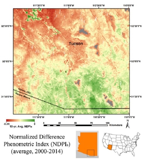
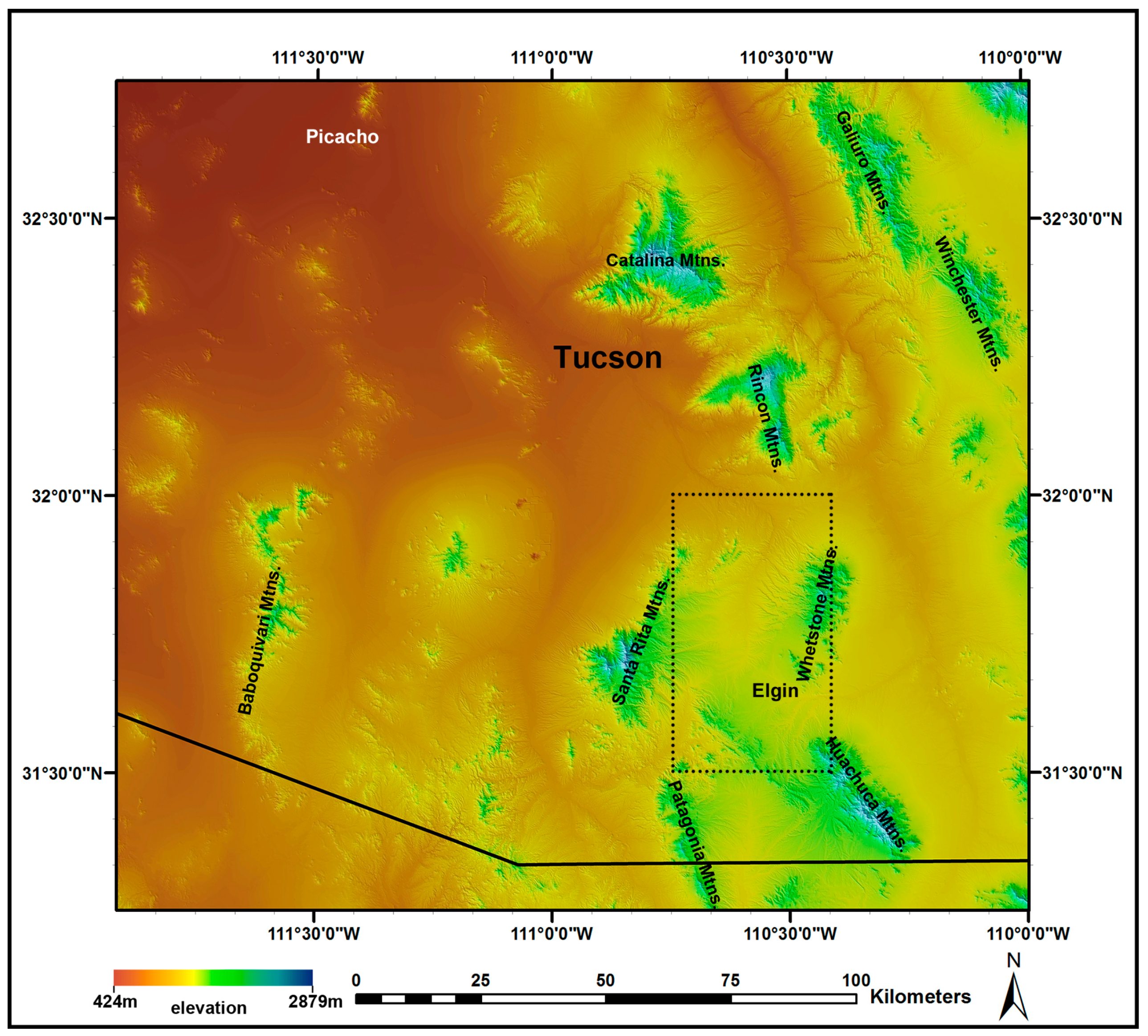
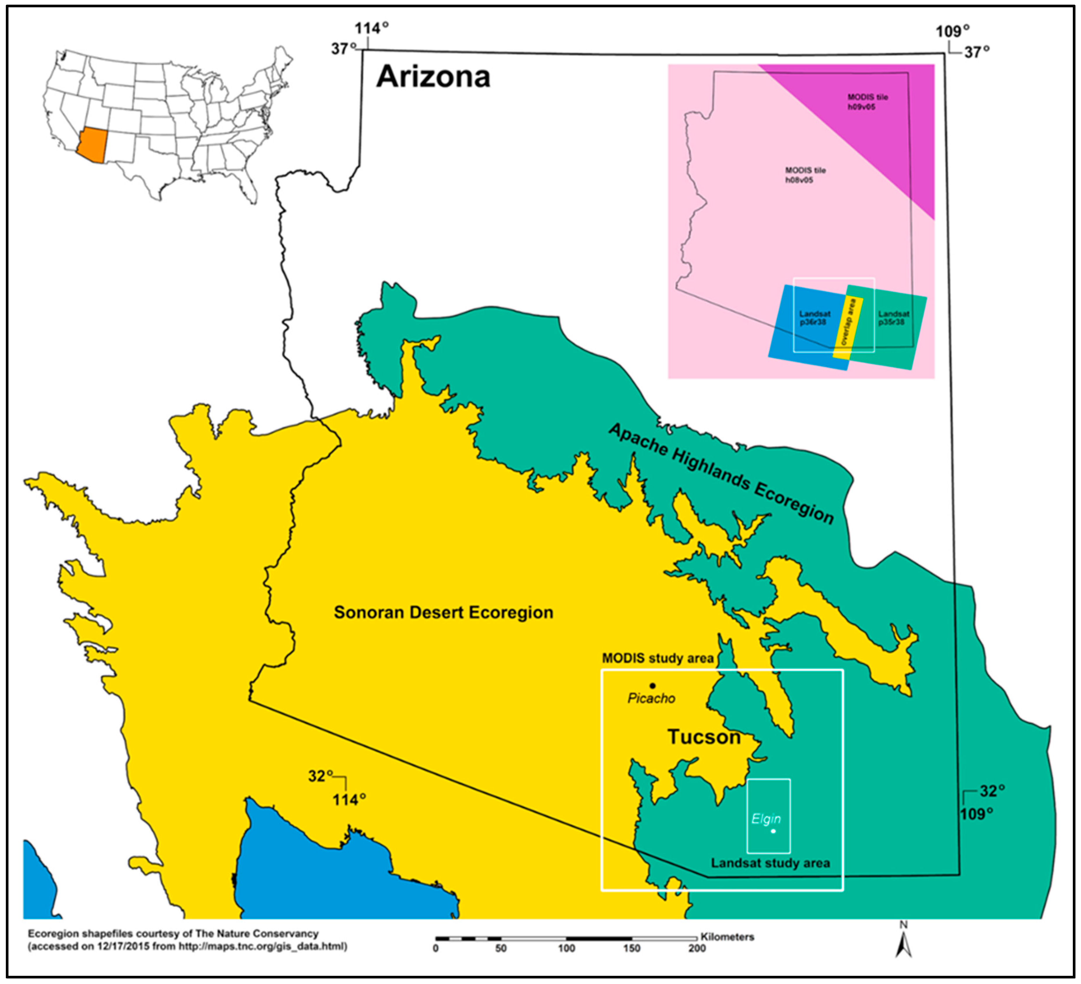
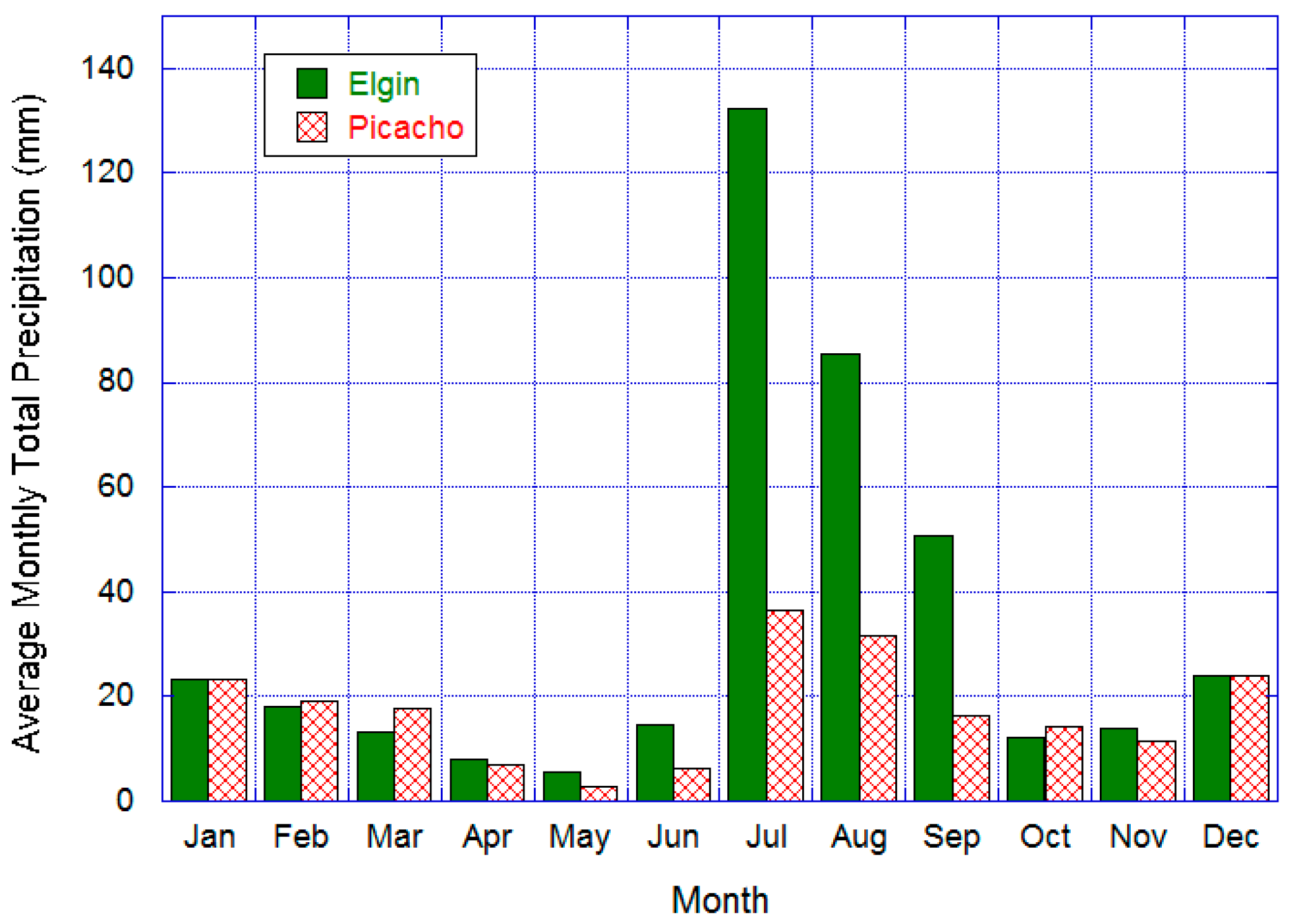
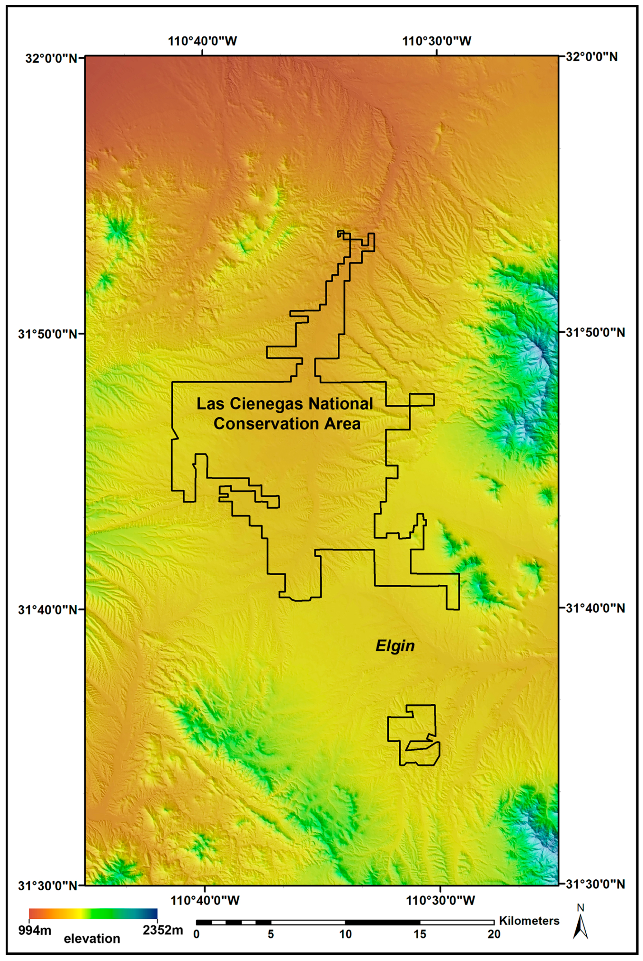
2.1. Study Area
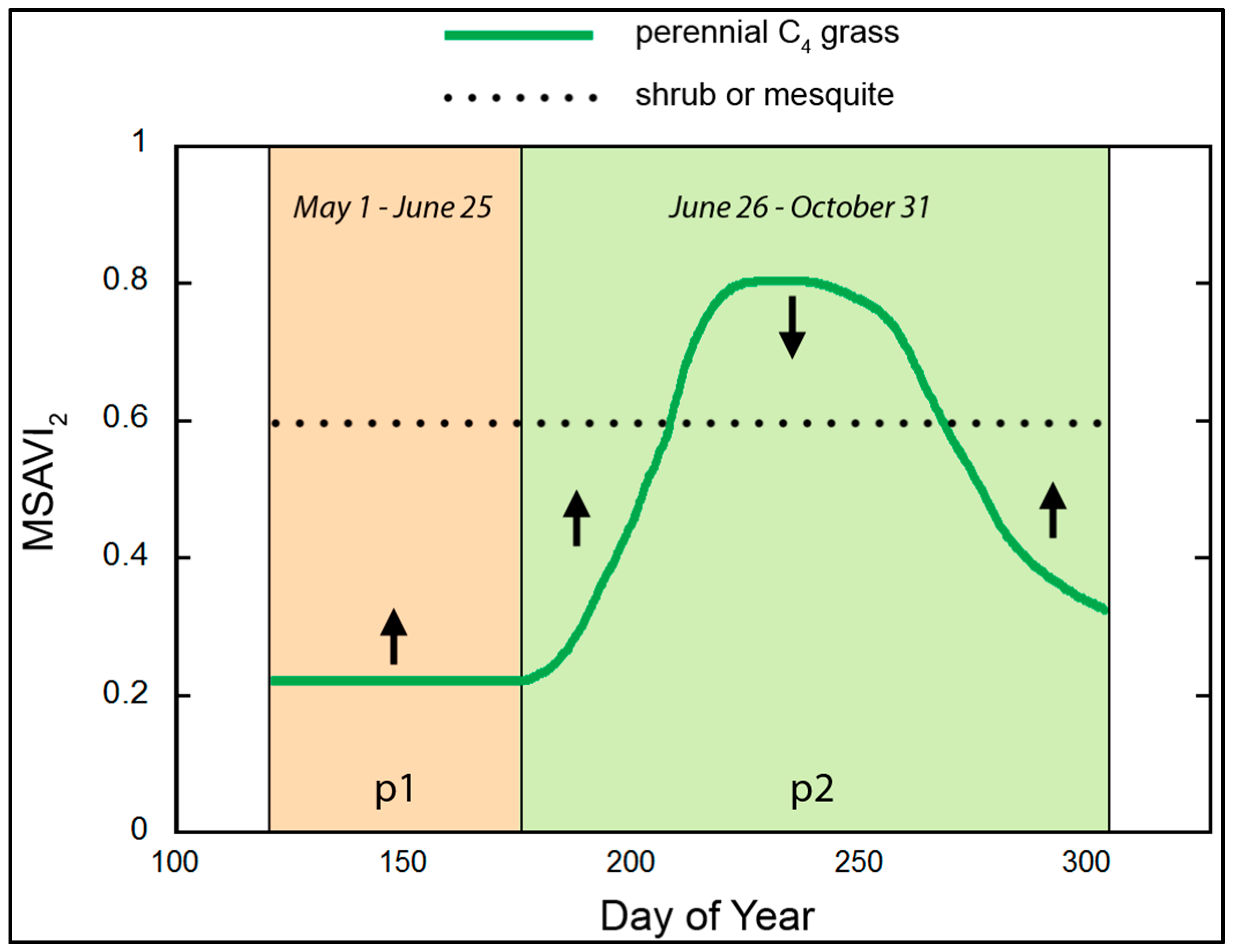
2.2. Conceptual Basis
2.3. Normalized Difference Phenometric Index
2.4. Specification of NDPI Parameters and Variables
2.5. Potential Variation in the NDPI-Vegetation Cover Relationship
2.6. Landsat Data and Analysis
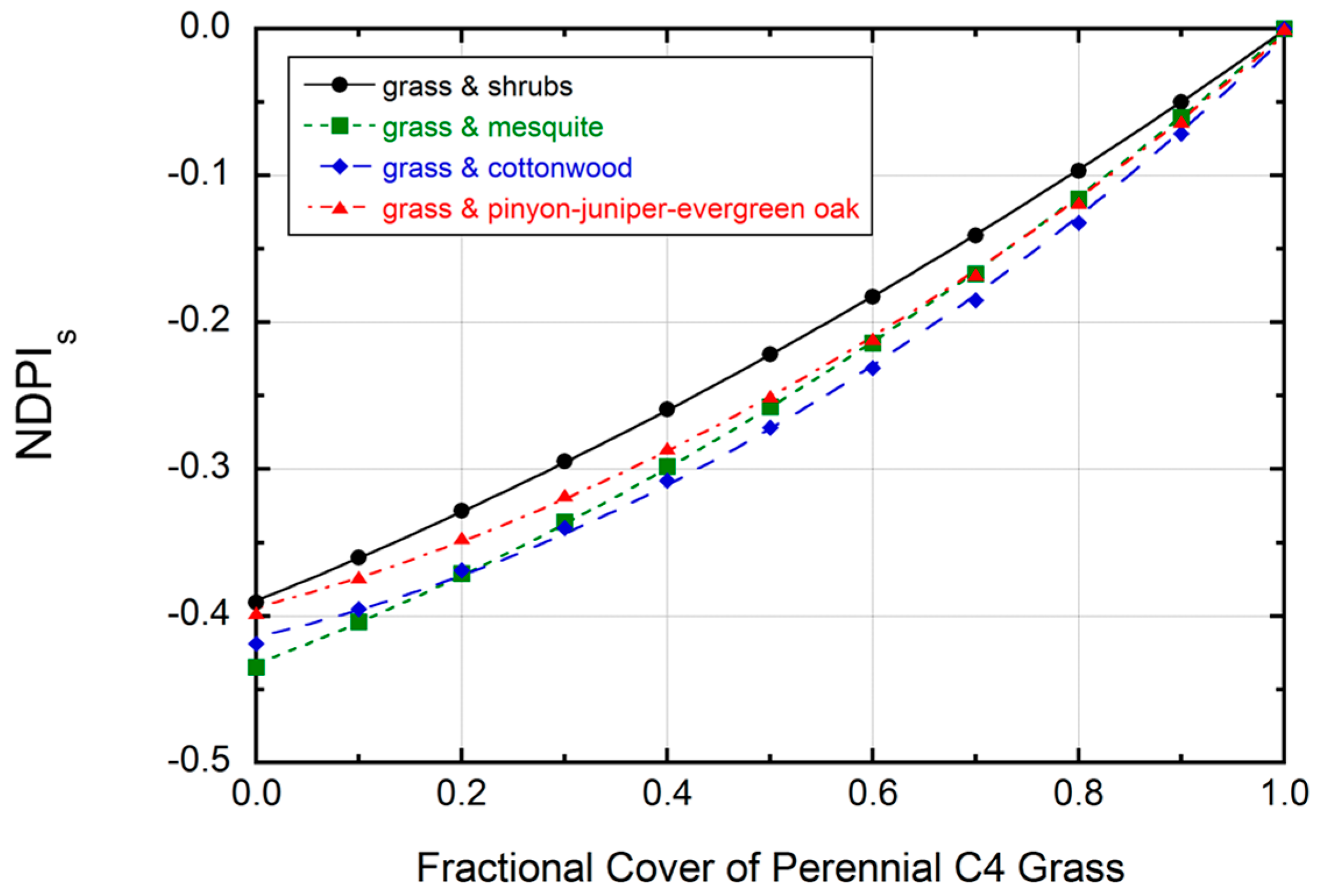
2.7. Numerical Modeling of NDPIs Response to Variation in Perennial C4 Grass Cover
2.8. MODIS Data and Analysis
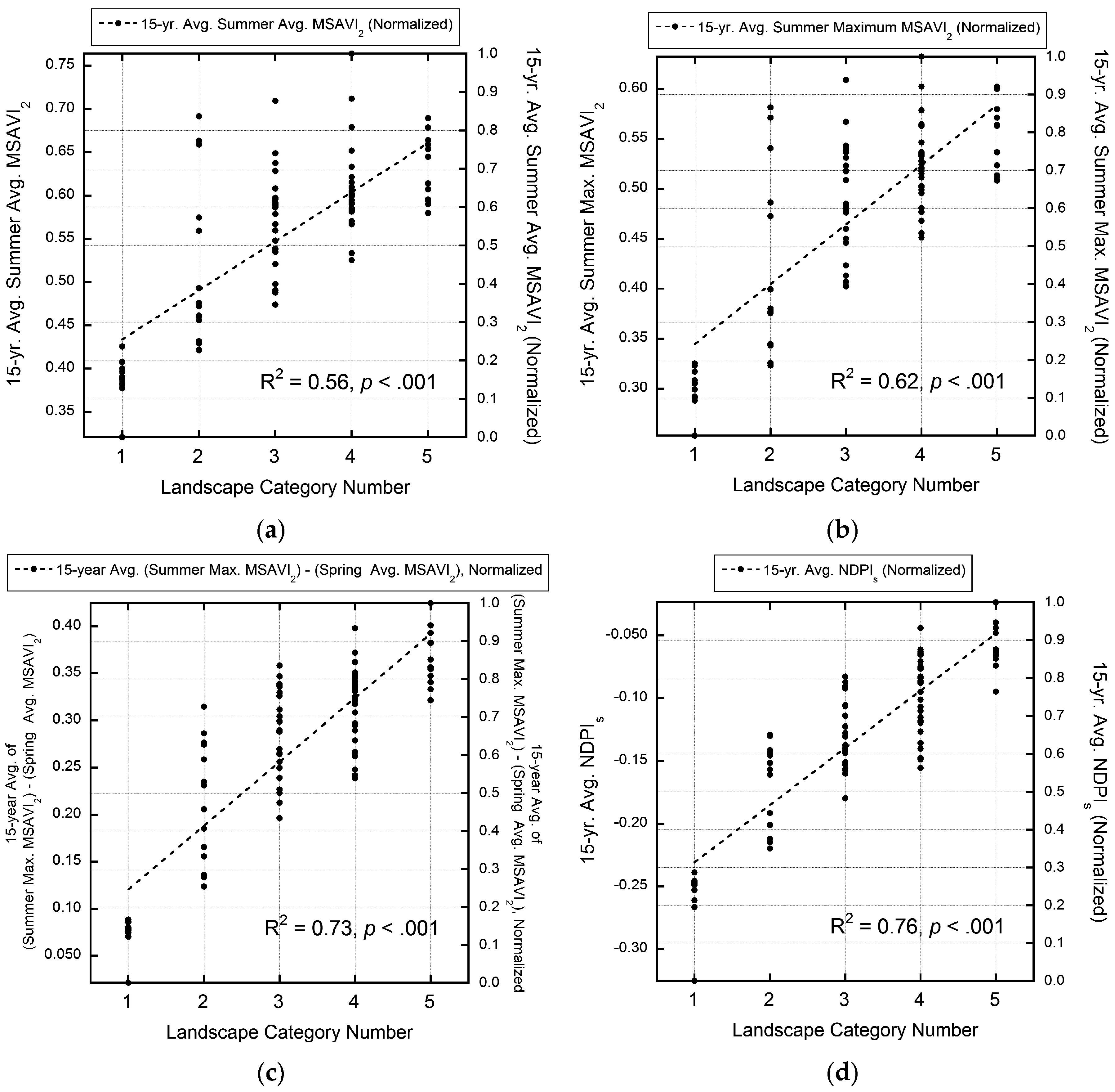
- summer average MSAVI2,
- summer maximum MSAVI2, and
- (summer maximum MSAVI2) − (spring average MSAVI2),
2.9. Field Observations for Validation of Map Results
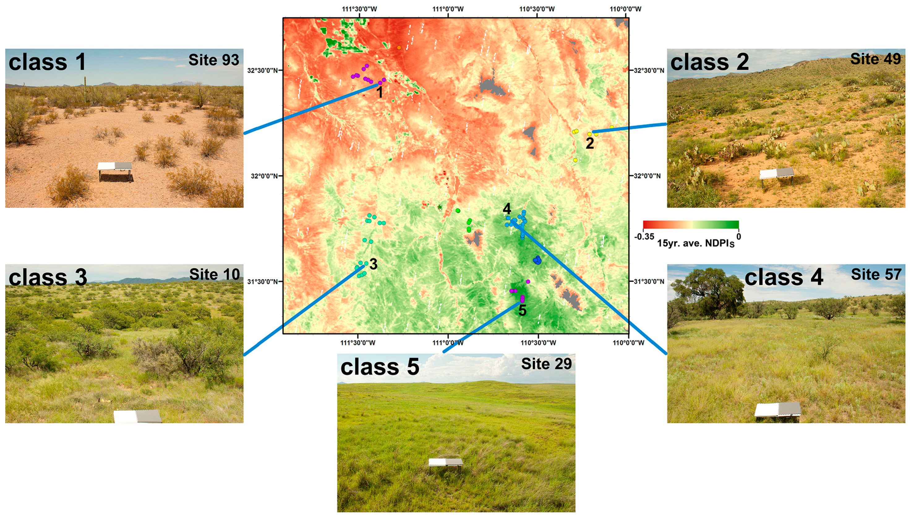
2.9.1. Data from Photographic Field Survey
- no grass cover (n = 11)
- minor grass cover (n = 15)
- moderate grass cover (n = 23)
- dense grass cover, with breaks (n = 31)
- dense, continuous grass cover (n = 12)
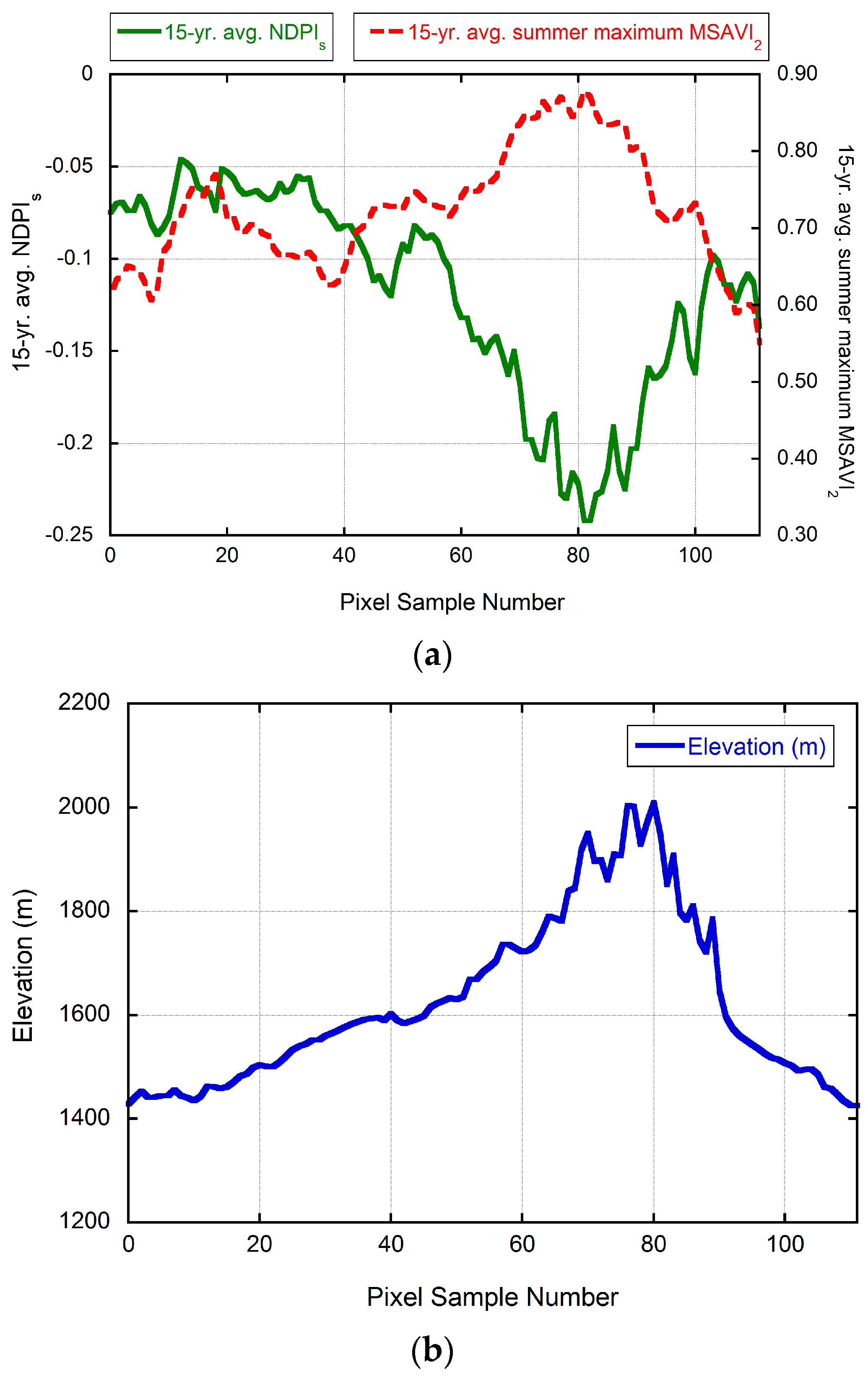
2.9.2. Data from Field Plots in a Sky Island Mountain Range
3. Results and Discussion
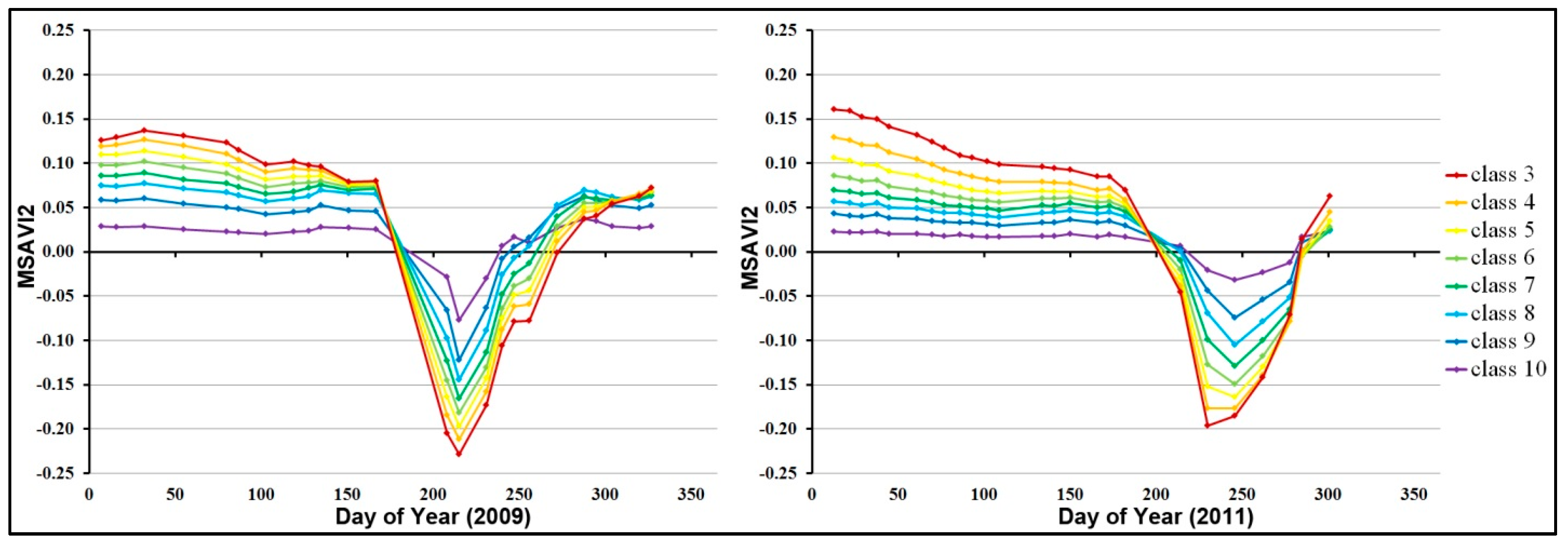
3.1. Landsat-Based Results
3.2. Numerical Modeling Results
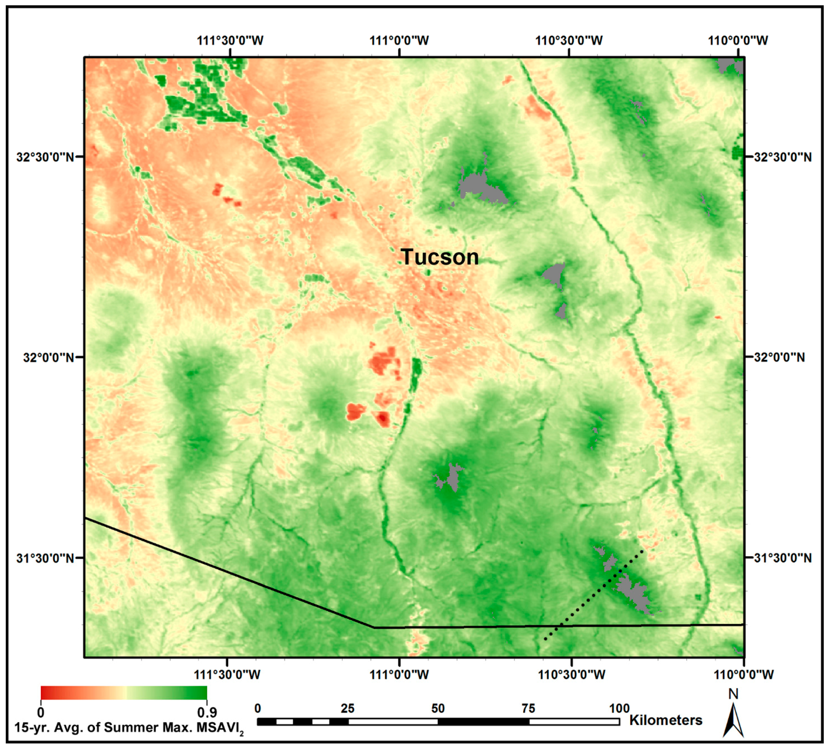
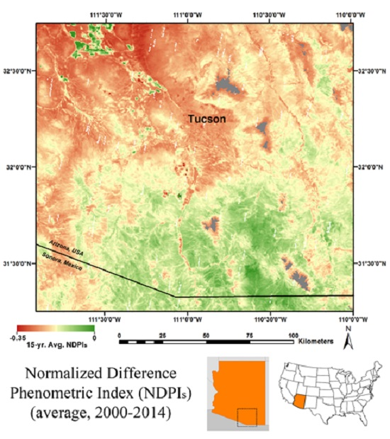
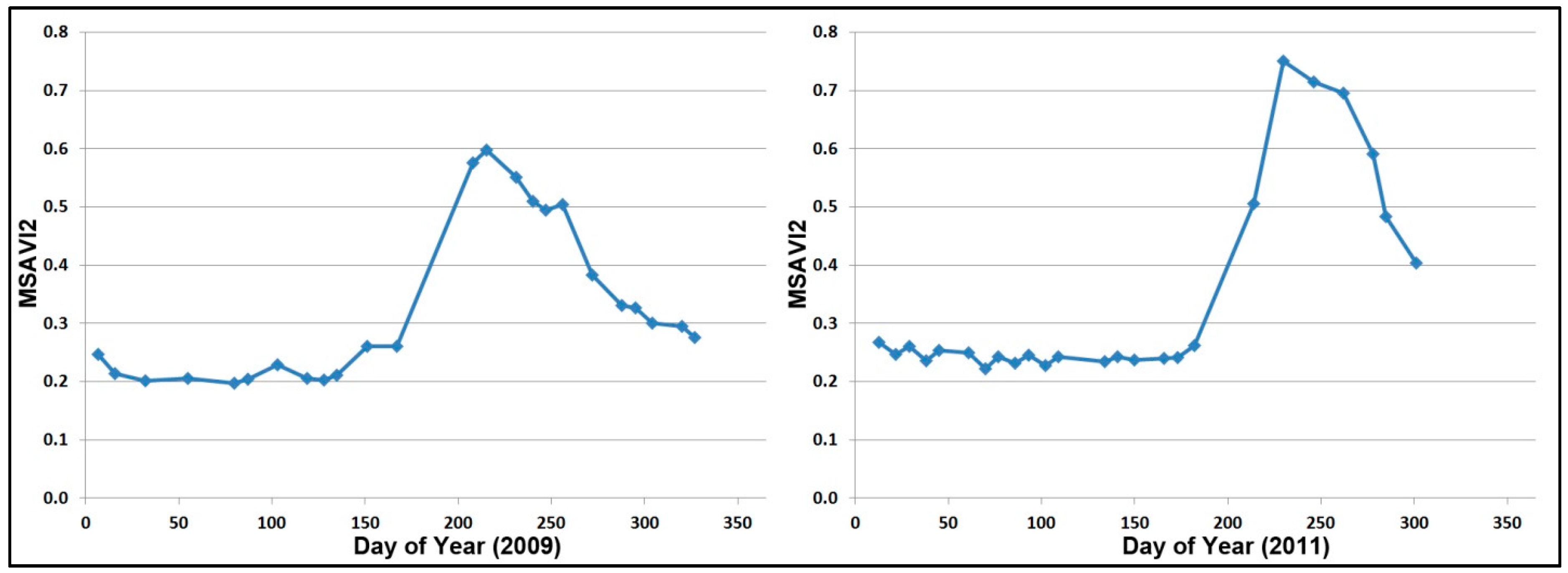
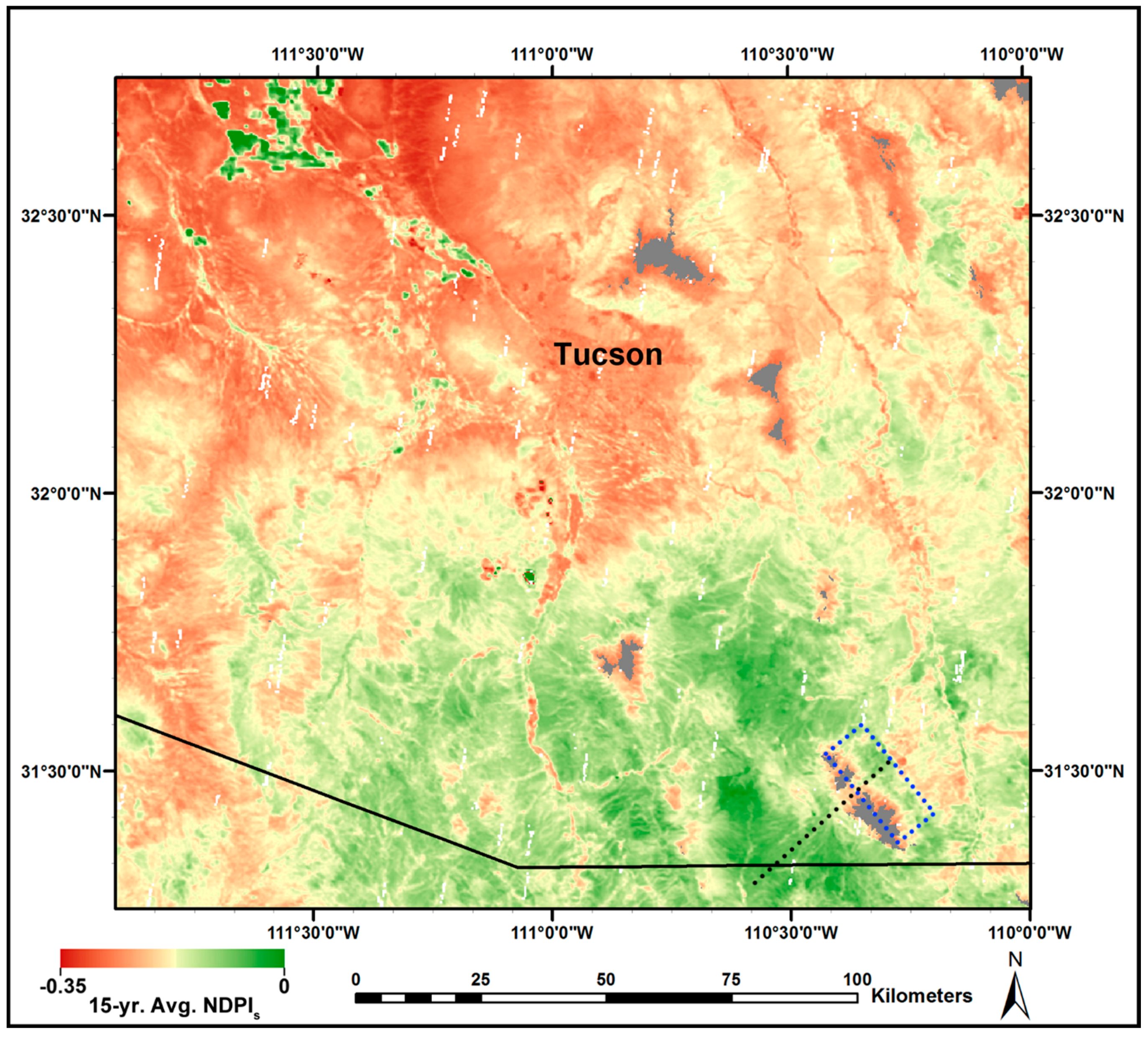
3.3. MODIS-Based Map Results
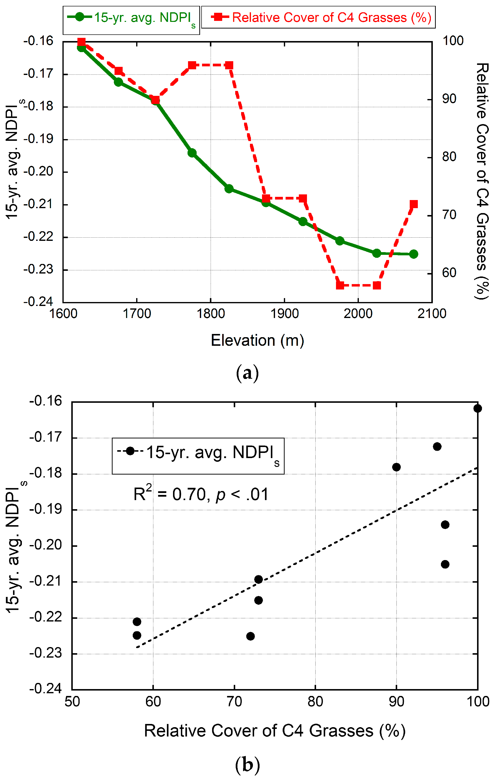
3.4. Validation of MODIS-Based Map Results
4. Conclusions
Supplementary Materials
Acknowledgments
Author Contributions
Conflicts of Interest
Abbreviations
| AVHRR | Advanced Very High Resolution Radiometer |
| BLM | Bureau of Land Management |
| DSLR | digital single-lens reflex |
| DVP | differential vegetation phenology |
| GPS | Global Positioning System |
| LCNCA | Las Cienegas National Conservation Area |
| MODIS | Moderate Resolution Imaging Spectroradiometer |
| MSAVI2 | modified soil-adjusted vegetation index |
| NDPI | normalized difference phenometric index |
| NDVI | normalized difference vegetation index |
| TM | Thematic Mapper |
| USGS | United States Geological Survey |
| VI | vegetation index |
References
- Nickerson, C.; Ebel, R.; Borchers, A.; Carriazo, F. Major Uses of Land in the United States, 2007; US Department of Agriculture, Economic Research Service: Washington, DC, USA, 2011.
- Van Auken, O.W. Shrub invasions of North American semiarid grasslands. Annu. Rev. Ecol. System. 2000, 31, 197–215. [Google Scholar] [CrossRef]
- Bahre, C.J.; Shelton, M.L. Rangeland destruction: Cattle and drought in southeastern Arizona at the turn of the century. J. Southwest 1996, 38, 1–22. [Google Scholar]
- Anable, M.E.; McClaran, M.P.; Ruyle, G.B. Spread of introduced Lehmann lovegrass Eragrostis lehmanniana Nees. in southern Arizona, USA. Biol. Conserv. 1992, 61, 181–188. [Google Scholar] [CrossRef]
- Fredrickson, E.; Havstad, K.M.; Estell, R.; Hyder, P. Perspectives on desertification: South-western United States. J. Arid Environ. 1998, 39, 191–207. [Google Scholar] [CrossRef]
- Holechek, J.; Galt, D.; Joseph, J.; Navarro, J.; Kumalo, G.; Molinar, F.; Thomas, M. Moderate and light cattle grazing effects on Chihuahuan Desert rangelands. J. Range Manag. 2003, 56, 133–139. [Google Scholar] [CrossRef]
- Hobbs, N.T.; Galvin, K.A.; Stokes, C.J.; Lackett, J.M.; Ash, A.J.; Boone, R.B.; Reid, R.S.; Thornton, P.K. Fragmentation of rangelands: Implications for humans, animals, and landscapes. Glob. Environ. Chang. 2008, 18, 776–785. [Google Scholar] [CrossRef]
- Marshall, R.M.; Turner, D.; Gondor, A.; Gori, D.; Enquist, C.; Luna, G.; Paredes Aguilar, R.; Anderson, S.; Schwartz, S.; Watts, C.; et al. An Ecological Analysis of Conservation Priorities in the Apache Highlands Ecoregion; The Nature Conservancy and Instituto del Medio Ambiente y el Desarrollo Sustentable del Estado de Sonora with support from agency and institutional partners: Tuscon, AZ, USA, 2004. [Google Scholar]
- Cingolani, A.M.; Noy-Meir, I.; Díaz, S. Grazing effects on rangeland diversity: A synthesis of contemporary models. Ecol. Appl. 2005, 15, 757–773. [Google Scholar] [CrossRef]
- Vetter, S. Rangelands at equilibrium and non-equilibrium: Recent developments in the debate. J. Arid Environ. 2005, 62, 321–341. [Google Scholar] [CrossRef]
- Swetnam, T.W.; Betancourt, J.L. Mesoscale disturbance and ecological response to decadal climatic variability in the American Southwest. In Tree Rings and Natural Hazards; Springer: Heidelberg, Germany, 2010; pp. 329–359. [Google Scholar]
- Weltzin, J.F.; McPherson, G.R. Implications of precipitation redistribution for shifts in temperate savanna ecotones. Ecology 2000, 81, 1902–1913. [Google Scholar] [CrossRef]
- Munson, S.M.; Webb, R.H.; Belnap, J.; Andrew Hubbard, J.; Swann, D.E.; Rutman, S. Forecasting climate change impacts to plant community composition in the Sonoran Desert region. Glob. Chang. Biol. 2012, 18, 1083–1095. [Google Scholar] [CrossRef]
- Gremer, J.R.; Bradford, J.B.; Munson, S.M.; Duniway, M.C. Desert grassland responses to climate and soil moisture suggest divergent vulnerabilities across the southwestern United States. Glob. Chang. Biol. 2015, 21, 4049–4062. [Google Scholar] [CrossRef] [PubMed]
- Asner, G.P.; Elmore, A.J.; Olander, L.P.; Martin, R.E.; Harris, A.T. Grazing systems, ecosystem responses, and global change. Annu. Rev. Environ. Resour. 2004, 29, 261–299. [Google Scholar] [CrossRef]
- Bestelmeyer, B.T.; Herrick, J.E.; Brown, J.R.; Trujillo, D.A.; Havstad, K.M. Land management in the American Southwest: A state-and-transition approach to ecosystem complexity. Environ. Manag. 2004, 34, 38–51. [Google Scholar] [CrossRef] [PubMed]
- Havstad, K.M.; Peters, D.P.; Skaggs, R.; Brown, J.; Bestelmeyer, B.; Fredrickson, E.; Herrick, J.; Wright, J. Ecological services to and from rangelands of the United States. Ecol. Econ. 2007, 64, 261–268. [Google Scholar] [CrossRef]
- Campbell, B.M.; Gordon, I.J.; Luckert, M.K.; Petheram, L.; Vetter, S. In search of optimal stocking regimes in semi-arid grazing lands: One size does not fit all. Ecol. Econ. 2006, 60, 75–85. [Google Scholar] [CrossRef]
- Milton, S.J.; du Plessis, M.A.; Siegfried, W.R. A conceptual model of arid rangeland degradation. Bioscience 1994, 44, 70–76. [Google Scholar] [CrossRef]
- Verger, A.; Filella, I.; Baret, F.; Peñuelas, J. Vegetation baseline phenology from kilometric global LAI satellite products. Remote Sens. Environ. 2016, 178, 1–14. [Google Scholar] [CrossRef]
- Nijland, W.; Bolton, D.K.; Coops, N.C.; Stenhouse, G. Imaging phenology; scaling from camera plots to landscapes. Remote Sens. Environ. 2016, 177, 13–20. [Google Scholar] [CrossRef]
- Dudley, K.L.; Dennison, P.E.; Roth, K.L.; Roberts, D.A.; Coates, A.R. A multi-temporal spectral library approach for mapping vegetation species across spatial and temporal phenological gradients. Remote Sens. Environ. 2015, 167, 121–134. [Google Scholar] [CrossRef]
- Bradley, B.A. Remote detection of invasive plants: A review of spectral, textural and phenological approaches. Biol. Invasions 2014, 16, 1411–1425. [Google Scholar] [CrossRef]
- Hüttich, C.; Gessner, U.; Herold, M.; Strohbach, B.J.; Schmidt, M.; Keil, M.; Dech, S. On the suitability of MODIS time series metrics to map vegetation types in dry savanna ecosystems: A case study in the Kalahari of NE Namibia. Remote Sens. 2009, 1, 620–643. [Google Scholar] [CrossRef]
- Brandt, M.; Hiernaux, P.; Tagesson, T.; Verger, A.; Rasmussen, K.; Diouf, A.A.; Mbow, C.; Mougin, E.; Fensholt, R. Woody plant cover estimation in drylands from Earth Observation based seasonal metrics. Remote Sens. Environ. 2016, 172, 28–38. [Google Scholar] [CrossRef]
- Blanco, L.J.; Paruelo, J.M.; Oesterheld, M.; Biurrun, F.N. Spatial and temporal patterns of herbaceous primary production in semi-arid shrublands: A remote sensing approach. J. Veg. Sci. 2016, 27, 716–727. [Google Scholar] [CrossRef]
- Bajocco, S.; Dragoz, E.; Gitas, I.; Smiraglia, D.; Salvati, L.; Ricotta, C. Mapping forest fuels through vegetation phenology: The role of coarse-resolution satellite time-series. PLoS ONE 2015, 10, e0119811. [Google Scholar] [CrossRef] [PubMed]
- Elmore, A.J.; Asner, G.P.; Hughes, R.F. Satellite monitoring of vegetation phenology and fire fuel conditions in Hawaiian drylands. Earth Interact. 2005, 9, 1–21. [Google Scholar] [CrossRef]
- Van Wagtendonk, J.W.; Root, R.R. The use of multi-temporal Landsat Normalized Difference Vegetation Index (NDVI) data for mapping fuel models in Yosemite National Park, USA. Int. J. Remote Sens. 2003, 24, 1639–1651. [Google Scholar] [CrossRef]
- Diouf, A.A.; Brandt, M.; Verger, A.; Jarroudi, M.E.; Djaby, B.; Fensholt, R.; Ndione, J.A.; Tychon, B. Fodder biomass monitoring in Sahelian rangelands using phenological metrics from FAPAR time series. Remote Sens. 2015, 7, 9122–9148. [Google Scholar] [CrossRef]
- Horion, S.; Cornet, Y.; Erpicum, M.; Tychon, B. Studying interactions between climate variability and vegetation dynamic using a phenology based approach. Int. J. Appl. Earth Obs. Geoinf. 2013, 20, 20–32. [Google Scholar] [CrossRef]
- Wu, C.; Gonsamo, A.; Chen, J.M.; Kurz, W.A.; Price, D.T.; Lafleur, P.M.; Jassal, R.S.; Dragoni, D.; Bohrer, G.; Gough, C.M. Interannual and spatial impacts of phenological transitions, growing season length, and spring and autumn temperatures on carbon sequestration: A North America flux data synthesis. Glob. Planet. Chang. 2012, 92, 179–190. [Google Scholar] [CrossRef]
- Cleland, E.E.; Chuine, I.; Menzel, A.; Mooney, H.A.; Schwartz, M.D. Shifting plant phenology in response to global change. Trends Ecol. Evol. 2007, 22, 357–365. [Google Scholar] [CrossRef] [PubMed]
- Pettorelli, N.; Vik, J.O.; Mysterud, A.; Gaillard, J.-M.; Tucker, C.J.; Stenseth, N.C. Using the satellite-derived NDVI to assess ecological responses to environmental change. Trends Ecol. Evol. 2005, 20, 503–510. [Google Scholar] [CrossRef] [PubMed]
- Weiss, J.L.; Gutzler, D.S.; Coonrod, J.E.A.; Dahm, C.N. Long-term vegetation monitoring with NDVI in a diverse semi-arid setting, central New Mexico, USA. J. Arid Environ. 2004, 58, 249–272. [Google Scholar] [CrossRef]
- Salinas-Zavala, C.; Douglas, A.; Diaz, H. Interannual variability of NDVI in northwest Mexico. Associated climatic mechanisms and ecological implications. Remote Sens. Environ. 2002, 82, 417–430. [Google Scholar] [CrossRef]
- White, M.A.; Thornton, P.E.; Running, S.W. A continental phenology model for monitoring vegetation responses to interannual climatic variability. Glob. Biogeochem. Cycles 1997, 11, 217–234. [Google Scholar] [CrossRef]
- Eklundh, L.; Jönsson, P. TIMESAT: A Software Package for Time-Series Processing and Assessment of Vegetation Dynamics. In Remote Sensing Time Series; Springer: Heidelberg, Germany, 2015; pp. 141–158. [Google Scholar]
- Verma, M.; Friedl, M.A.; Finzi, A.; Phillips, N. Multi-criteria evaluation of the suitability of growth functions for modeling remotely sensed phenology. Ecol. Model. 2016, 323, 123–132. [Google Scholar] [CrossRef]
- Tan, B.; Morisette, J.T.; Wolfe, R.E.; Gao, F.; Ederer, G.A.; Nightingale, J.; Pedelty, J.A. An enhanced TIMESAT algorithm for estimating vegetation phenology metrics from MODIS data. IEEE J. Sel. Top. Appl. Earth Obs. Remote Sens. 2011, 4, 361–371. [Google Scholar] [CrossRef]
- Wu, J.; Albert, L.P.; Lopes, A.P.; Restrepo-Coupe, N.; Hayek, M.; Wiedemann, K.T.; Guan, K.; Stark, S.C.; Christoffersen, B.; Prohaska, N.; et al. Leaf development and demography explain photosynthetic seasonality in Amazon evergreen forests. Science 2016, 351, 972–976. [Google Scholar] [CrossRef] [PubMed]
- Suzuki, R.; Kobayashi, H.; Delbart, N.; Asanuma, J.; Hiyama, T. NDVI responses to the forest canopy and floor from spring to summer observed by airborne spectrometer in eastern Siberia. Remote Sens. Environ. 2011, 115, 3615–3624. [Google Scholar] [CrossRef]
- Ahl, D.E.; Gower, S.T.; Burrows, S.N.; Shabanov, N.V.; Myneni, R.B.; Knyazikhin, Y. Monitoring spring canopy phenology of a deciduous broadleaf forest using MODIS. Remote Sens. Environ. 2006, 104, 88–95. [Google Scholar] [CrossRef]
- Kobayashi, H.; Delbart, N.; Suzuki, R.; Kushida, K. A satellite-based method for monitoring seasonality in the overstory leaf area index of Siberian larch forest. J. Geophys. Res. Biogeosci. 2010, 115, 30–31. [Google Scholar] [CrossRef]
- Moody, A.; Johnson, D.M. Land-surface phenologies from AVHRR using the discrete Fourier transform. Remote Sens. Environ. 2001, 75, 305–323. [Google Scholar] [CrossRef]
- Hirosawa, Y.; Marsh, S.E.; Kliman, D.H. Application of standardized principal component analysis to land-cover characterization using multitemporal AVHRR data. Remote Sens. Environ. 1996, 58, 267–281. [Google Scholar] [CrossRef]
- Roderick, M.L.; Noble, I.R.; Cridland, S.W. Estimating woody and herbaceous vegetation cover from time series satellite observations. Glob. Ecol. Biogeogr. 1999, 8, 501–508. [Google Scholar] [CrossRef]
- Lu, H.; Raupach, M.R.; McVicar, T.R.; Barrett, D.J. Decomposition of vegetation cover into woody and herbaceous components using AVHRR NDVI time series. Remote Sens. Environ. 2003, 86, 1–18. [Google Scholar] [CrossRef]
- Cleveland, R.B.; Cleveland, W.S.; McRae, J.E.; Terpenning, I. STL: A seasonal-trend decomposition procedure based on loess. J. Off. Stat. 1990, 6, 3–73. [Google Scholar]
- Pisek, J.; Rautiainen, M.; Nikopensius, M.; Raabe, K. Estimation of seasonal dynamics of understory NDVI in northern forests using MODIS BRDF data: Semi-empirical versus physically-based approach. Remote Sens. Environ. 2015, 163, 42–47. [Google Scholar] [CrossRef]
- Yang, W.; Kobayashi, H.; Suzuki, R.; Nasahara, K. A simple method for retrieving understory NDVI in sparse needleleaf forests in Alaska using MODIS BRDF data. Remote Sens. 2014, 6, 11936–11955. [Google Scholar] [CrossRef]
- Pisek, J.; Chen, J.M.; Miller, J.R.; Freemantle, J.R.; Peltoniemi, J.I.; Simic, A. Mapping forest background reflectance in a boreal region using multiangle compact airborne spectrographic imager data. IEEE Trans. Geosci. Remote Sens. 2010, 48, 499–510. [Google Scholar] [CrossRef]
- Scanlon, T.M.; Albertson, J.D.; Caylor, K.K.; Williams, C.A. Determining land surface fractional cover from NDVI and rainfall time series for a savanna ecosystem. Remote Sens. Environ. 2002, 82, 376–388. [Google Scholar] [CrossRef]
- Johnson, B.; Tateishi, R.; Kobayashi, T. Remote sensing of fractional green vegetation cover using spatially-interpolated endmembers. Remote Sens. 2012, 4, 2619–2634. [Google Scholar] [CrossRef]
- Gessner, U.; Klein, D.; Conrad, C.; Schmidt, M.; Dech, S. Towards an automated estimation of vegetation cover fractions on multiple scales: Examples of Eastern and Southern Africa. In Proceedings of the 33rd International Symposium on Remote Sensing of Environment, Stresa, Italy, 4–8 May 2009.
- Helman, D.; Lensky, I.M.; Tessler, N.; Osem, Y. A phenology-based method for monitoring woody and herbaceous vegetation in mediterranean forests from NDVI time series. Remote Sens. 2015, 7, 12314–12335. [Google Scholar] [CrossRef]
- Chakroun, H.; Mouillot, F.; Hamdi, A. Regional equivalent water thickness modeling from remote sensing across a tree cover/LAI gradient in Mediterranean forests of northern Tunisia. Remote Sens. 2015, 7, 1937–1961. [Google Scholar] [CrossRef]
- Blair, J.; Nippert, J.; Briggs, J. Grassland Ecology. In Ecology and the Environment; Springer: Heidelberg, Germany, 2014; pp. 389–423. [Google Scholar]
- Breshears, D.D.; Barnes, F.J. Interrelationships between plant functional types and soil moisture heterogeneity for semiarid landscapes within the grassland/forest continuum: A unified conceptual model. Landsc. Ecol. 1999, 14, 465–478. [Google Scholar] [CrossRef]
- Weltzin, J.F.; McPherson, G.R. Spatial and temporal soil moisture resource partitioning by trees and grasses in a temperate savanna, Arizona, USA. Oecologia 1997, 112, 156–164. [Google Scholar] [CrossRef]
- Burgess, T.L. Desert grassland, mixed shrub savanna, shrub steppe, or semidesert scrub. In The Desert Grassland; Burgess, T.L., McClaran, M., Van Devender, T., Eds.; University of Arizona Press: Tucson, AZ, USA, 1995; pp. 31–67. [Google Scholar]
- Cable, D.R. Influence of precipitation on perennial grass production in the semidesert southwest. Ecology 1975, 56, 981–986. [Google Scholar] [CrossRef]
- Fowler, N. The role of competition in plant communities in arid and semiarid regions. Annu. Rev. Ecol. Syst. 1986, 17, 89–110. [Google Scholar] [CrossRef]
- Sandquist, D.R. Plants in Desert Environments; Springer: New York, NY, USA, 2014; pp. 1–25. [Google Scholar]
- Yuan, W.; Zhou, G.; Wang, Y.; Han, X.; Wang, Y. Simulating phenological characteristics of two dominant grass species in a semi-arid steppe ecosystem. Ecol. Res. 2007, 22, 784–791. [Google Scholar] [CrossRef]
- Kemp, P.R. Phenological patterns of Chihuahuan Desert plants in relation to the timing of water availability. J. Ecol. 1983, 71, 427–436. [Google Scholar] [CrossRef]
- Forzieri, G.; Castelli, F.; Vivoni, E.R. Vegetation dynamics within the North American monsoon region. J. Clim. 2011, 24, 1763–1783. [Google Scholar] [CrossRef]
- Van Leeuwen, W.J.; Davison, J.E.; Casady, G.M.; Marsh, S.E. Phenological characterization of desert sky island vegetation communities with remotely sensed and climate time series data. Remote Sens. 2010, 2, 388–415. [Google Scholar] [CrossRef]
- Walker, J.; De Beurs, K.; Wynne, R. Dryland vegetation phenology across an elevation gradient in Arizona, USA, investigated with fused MODIS and Landsat data. Remote Sens. Environ. 2014, 144, 85–97. [Google Scholar] [CrossRef]
- Enquist, C.A.; Gori, D.F. Application of an expert system approach for assessing grassland status in the US-Mexico borderlands: Implications for conservation and management. Nat. Areas J. 2008, 28, 414–428. [Google Scholar] [CrossRef]
- Franklin, J.; Turner, D.L. The application of a geometric optical canopy reflectance model to semiarid shrub vegetation. IEEE Trans. Geosci. Remote Sens. 1992, 30, 293–301. [Google Scholar] [CrossRef]
- Adams, D.K.; Comrie, A.C. The north American monsoon. Bull. Am. Meteorol. Soc. 1997, 78, 2197–2213. [Google Scholar] [CrossRef]
- Sheppard, P.; Comrie, A.; Packin, G.D.; Angersbach, K.; Hughes, M. The climate of the US Southwest. Clim. Res. 2002, 21, 219–238. [Google Scholar] [CrossRef]
- Lowe, C.H. The Vertebrates of Arizona; University of Arizona Press: Tucson, AZ, USA, 1964; p. 270. [Google Scholar]
- Menne, M.; Durre, I.; Korzeniewski, B.; McNeal, S.; Thomas, K.; Yin, X.; Anthony, S.; Ray, R.; Vose, R.; Gleason, B. Global Historical Climatology Network-Daily (GHCN-Daily), Version 3; NOAA National Climatic Data Center: Asheville, NC, USA, 2012.
- Chesson, P.; Gebauer, R.L.; Schwinning, S.; Huntly, N.; Wiegand, K.; Ernest, M.S.; Sher, A.; Novoplansky, A.; Weltzin, J.F. Resource pulses, species interactions, and diversity maintenance in arid and semi-arid environments. Oecologia 2004, 141, 236–253. [Google Scholar] [CrossRef] [PubMed]
- Ehleringer, J. Annuals and perennials of warm deserts. In Physiological Ecology of North American Plant Communities; Springer: Heidelberg, Germany, 1985; pp. 162–180. [Google Scholar]
- Hamerlynck, E.P.; Scott, R.L.; Moran, M.S.; Keefer, T.O.; Huxman, T.E. Growing season ecosystem and leaf-level gas exchange of an exotic and native semiarid bunchgrass. Oecologia 2010, 163, 561–570. [Google Scholar] [CrossRef] [PubMed]
- Schenk, H.J.; Jackson, R.B. Rooting depths, lateral root spreads and below-ground/above-ground allometries of plants in water-limited ecosystems. J. Ecol. 2002, 90, 480–494. [Google Scholar] [CrossRef]
- Sanchez-Mejia, Z.M.; Papuga, S.A.; Swetish, J.B.; van Leeuwen, W.J.D.; Szutu, D.; Hartfield, K. Quantifying the influence of deep soil moisture on ecosystem albedo: The role of vegetation. Water Resour. Res. 2014, 50, 4038–4053. [Google Scholar] [CrossRef]
- Bajocco, S.; Rosati, L.; Ricotta, C. Knowing fire incidence through fuel phenology: A remotely sensed approach. Ecol. Model. 2010, 221, 59–66. [Google Scholar] [CrossRef]
- Jackson, R.D.; Huete, A.R. Interpreting vegetation indices. Prev. Vet. Med. 1991, 11, 185–200. [Google Scholar] [CrossRef]
- Liu, Z.Y.; Huang, J.F.; Wu, X.H.; Dong, Y.P. Comparison of vegetation indices and red-edge parameters for estimating grassland cover from canopy reflectance data. J. Integr. Plant Biol. 2007, 49, 299–306. [Google Scholar] [CrossRef]
- Qi, J.; Chehbouni, A.; Huete, A.; Kerr, Y.; Sorooshian, S. A modified soil adjusted vegetation index. Remote Sens. Environ. 1994, 48, 119–126. [Google Scholar] [CrossRef]
- Wentworth, T. Distributions of C4 plants along environmental and compositional gradients in southeastern Arizona. Vegetatio 1983, 52, 21–34. [Google Scholar]
- Hanan, N.; Prince, S.; Hiernaux, P. Spectral modelling of multicomponent landscapes in the Sahel. Int. J. Remote Sens. 1991, 12, 1243–4258. [Google Scholar] [CrossRef]
- Jiang, Z.; Huete, A.R. Linearization of NDVI based on its relationship with vegetation fraction. Photogramm. Eng. Remote Sens. 2010, 76, 965–975. [Google Scholar] [CrossRef]
- United States Geological Survey. Product Guide: Landsat 4-7 Climate Data Record (CDR), Surface Reflectance; USGS: Washington, DC, USA, 2015; p. 27.
- White, K.; Pontius, J.; Schaberg, P. Remote sensing of spring phenology in northeastern forests: A comparison of methods, field metrics and sources of uncertainty. Remote Sens. Environ. 2014, 148, 97–107. [Google Scholar] [CrossRef]
- Vogelmann, J.E.; Xian, G.; Homer, C.; Tolk, B. Monitoring gradual ecosystem change using Landsat time series analyses: Case studies in selected forest and rangeland ecosystems. Remote Sens. Environ. 2012, 122, 92–105. [Google Scholar] [CrossRef]
- Gori, D.; Schussman, H. State of the Las Cienegas National Conservation Area. Part I. Condition and Trend of the Desert Grassland and Watershed; The Nature Conservancy of Arizona: Tucson, AZ, USA, 2005. [Google Scholar]
- Bureau of Land Management. Las Cienegas National Conservation Area Manager's Annual Report FY 2014; BLM: Washington, DC, USA, 2015; pp. 1–31.
- Paruelo, J.M.; Lauenroth, W.K. Interannual variability of NDVI and its relationship to climate for North American shrublands and grasslands. J. Biogeogr. 1998, 25, 721–733. [Google Scholar] [CrossRef]
- Vermote, E.; Roger, J.; Ray, J. MODIS Surface Reflectance User’s Guide; Version 1.4; MODIS Land Surface Reflectance Science Computing Facility: Greenbelt, MD, USA, 2015. [Google Scholar]
- Towne, D.C.; Stephenson, L.W. Ambient Groundwater Quality of the San Rafael Basin: A 2002 Baseline Study; ADEQ Water Quality Division, Hydologic Support & Assessment Section, Groundwater Monitoring Unit: Phoenix, AZ, USA, 2003.
- McLaughlin, S.P. Vascular floras of Sonoita Creek State Natural Area and San Rafael State Park: Arizona’s first natural-area parks. SIDA Contrib. Bot. 2006, 22, 661–704. [Google Scholar]
- Olsen, J.; Miehe, S.; Ceccato, P.; Fensholt, R. Does EO NDVI seasonal metrics capture variations in species composition and biomass due to grazing in semi-arid grassland savannas? Biogeosciences 2015, 12, 4407–4419. [Google Scholar] [CrossRef]
- Goward, S.N.; Tucker, C.J.; Dye, D.G. North American vegetation patterns observed with the NOAA-7 advanced very high resolution radiometer. Vegetatio 1985, 64, 3–14. [Google Scholar] [CrossRef]
- Wentworth, T.R. Vegetation on limestone in the Huachuca Mountains, Arizona. Southwest. Nat. 1985, 30, 385–395. [Google Scholar] [CrossRef]
- Stephenson, N.L. Climatic control of vegetation distribution: The role of the water balance. Am. Nat. 1990, 135, 649–670. [Google Scholar] [CrossRef]
- Nguyen, U.; Glenn, E.P.; Nagler, P.L.; Scott, R.L. Long-term decrease in satellite vegetation indices in response to environmental variables in an iconic desert riparian ecosystem: The Upper San Pedro, Arizona, United States. Ecohydrology 2015, 8, 610–625. [Google Scholar] [CrossRef]
- Scott, R.L.; Shuttleworth, W.J.; Goodrich, D.C.; Maddock, T., III. The water use of two dominant vegetation communities in a semiarid riparian ecosystem. Agric. For. Meteorol. 2000, 105, 241–256. [Google Scholar] [CrossRef]
- Villarreal, M.; Drake, S.; Marsh, S.; McCoy, A. The influence of wastewater subsidy, flood disturbance and neighboring land use on current and historical patterns of riparian vegetation in a semi-arid watershed. River Res. Appl. 2012, 28, 1230–1245. [Google Scholar] [CrossRef]


| Common Name | Genus | Species | Life Form 1 | Photosynthetic Pathway |
|---|---|---|---|---|
| Native | ||||
| black grama | Bouteloua | eriopoda | P | C4 |
| blue grama | Bouteloua | gracilis | P | C4 |
| sideoats grama | Bouteloua | curtipendula | P | C4 |
| slender grama | Bouteloua | repens | P | C4 |
| hairy grama | Bouteloua | hirsuta | P | C4 |
| plains lovegrass | Eragrostis | intermedia | P | C4 |
| plains bristlegrass | Setaria | leucopila | P | C4 |
| sand dropseed | Sporobolus | cryptandrus | P | C4 |
| Arizona cottontop | Digitaria | californica | P | C4 |
| red three-awn | Aristida | purpurea | P | C4 |
| other three-awn species | Aristida | various | P | C4 |
| ring muhly | Muhlenbergia | torreyi | P | C4 |
| other muhly species | Muhlenbergia | various | P | C4 |
| fluff-grass | Dasyochloa | pulchella | P | C4 |
| tobosa grass | Pleuraphis | mutica | P | C4 |
| needlegrass species | Stipa | various | A | C 3 |
| alkali sacaton | Sporobolus | airoides | P | C4 |
| dropseed species | Sporobolus | various | P | C4 |
| sprangletop species | Leptochloa | various | P | C4 |
| Invasive | ||||
| red brome | Bromus | rubens | A | C4 |
| cheatgrass | Bromus | tectorum | A | C 3 |
| buffelgrass | Cenchrus | ciliaris | P | C4 |
| Lehmann lovegrass | Eragrostis | lehmanniana | P | C4 |
| weeping lovegrass | Eragrostis | curvula | P | C4 |
| Vegetation Component | Average MSAVI2 from Landsat for Dates in 2009 | |
|---|---|---|
| p1 | p2 | |
| perennial C4 grass | 0.23 | 0.57 |
| shrubs | 0.54 | 0.57 |
| mesquite | 0.66 | 0.64 |
| cottonwood (riparian) | 0.74 | 0.74 |
| pinyon-juniper-evergreen oak | 0.67 | 0.70 |
| 15-Year Avg. Data Product | Interval from Reference Landscape Category Number | |||||||
|---|---|---|---|---|---|---|---|---|
| +1 | +2 | +3 | Combined | |||||
| Avg. Overlap | (%) | Avg. Overlap | (%) | Avg. Overlap | (%) | Avg. Overlap | (%) | |
| Summer Average MSAVI2 | 0.33 | (64) | 0.22 | (48) | 0.13 | (35) | 0.23 | (49) |
| Summer Maximum MSAVI2 | 0.30 | (61) | 0.20 | (45) | 0.10 | (27) | 0.20 | (44) |
| (Summer Max. MSAVI2) − (Spring Avg. MSAVI2) | 0.19 | (54) | 0.09 | (24) | 0.00 | (0) | 0.10 | (26) |
| NDPIs | 0.14 | (49) | 0.04 | (14) | 0.00 | (0) | 0.06 | (21) |
© 2016 by the authors; licensee MDPI, Basel, Switzerland. This article is an open access article distributed under the terms and conditions of the Creative Commons Attribution (CC-BY) license (http://creativecommons.org/licenses/by/4.0/).
Share and Cite
Dye, D.G.; Middleton, B.R.; Vogel, J.M.; Wu, Z.; Velasco, M. Exploiting Differential Vegetation Phenology for Satellite-Based Mapping of Semiarid Grass Vegetation in the Southwestern United States and Northern Mexico. Remote Sens. 2016, 8, 889. https://doi.org/10.3390/rs8110889
Dye DG, Middleton BR, Vogel JM, Wu Z, Velasco M. Exploiting Differential Vegetation Phenology for Satellite-Based Mapping of Semiarid Grass Vegetation in the Southwestern United States and Northern Mexico. Remote Sensing. 2016; 8(11):889. https://doi.org/10.3390/rs8110889
Chicago/Turabian StyleDye, Dennis G., Barry R. Middleton, John M. Vogel, Zhuoting Wu, and Miguel Velasco. 2016. "Exploiting Differential Vegetation Phenology for Satellite-Based Mapping of Semiarid Grass Vegetation in the Southwestern United States and Northern Mexico" Remote Sensing 8, no. 11: 889. https://doi.org/10.3390/rs8110889