
InSAR Observation and Numerical Modeling of the Earth-Dam Displacement of Shuibuya Dam (China)


Abstract
:
1. Introduction
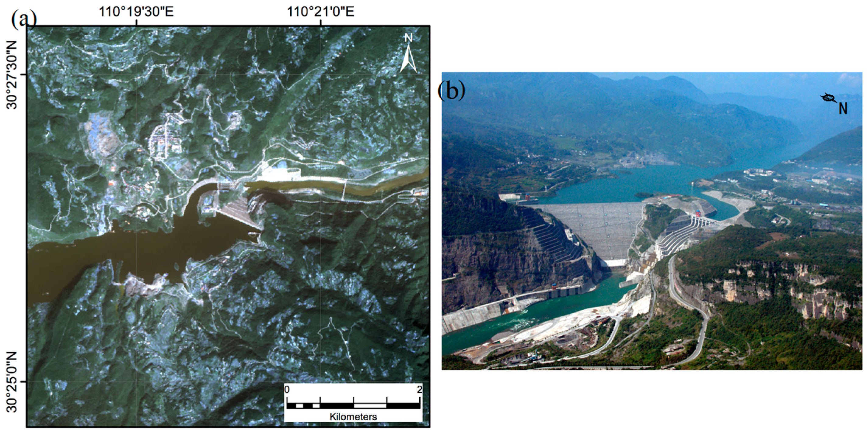
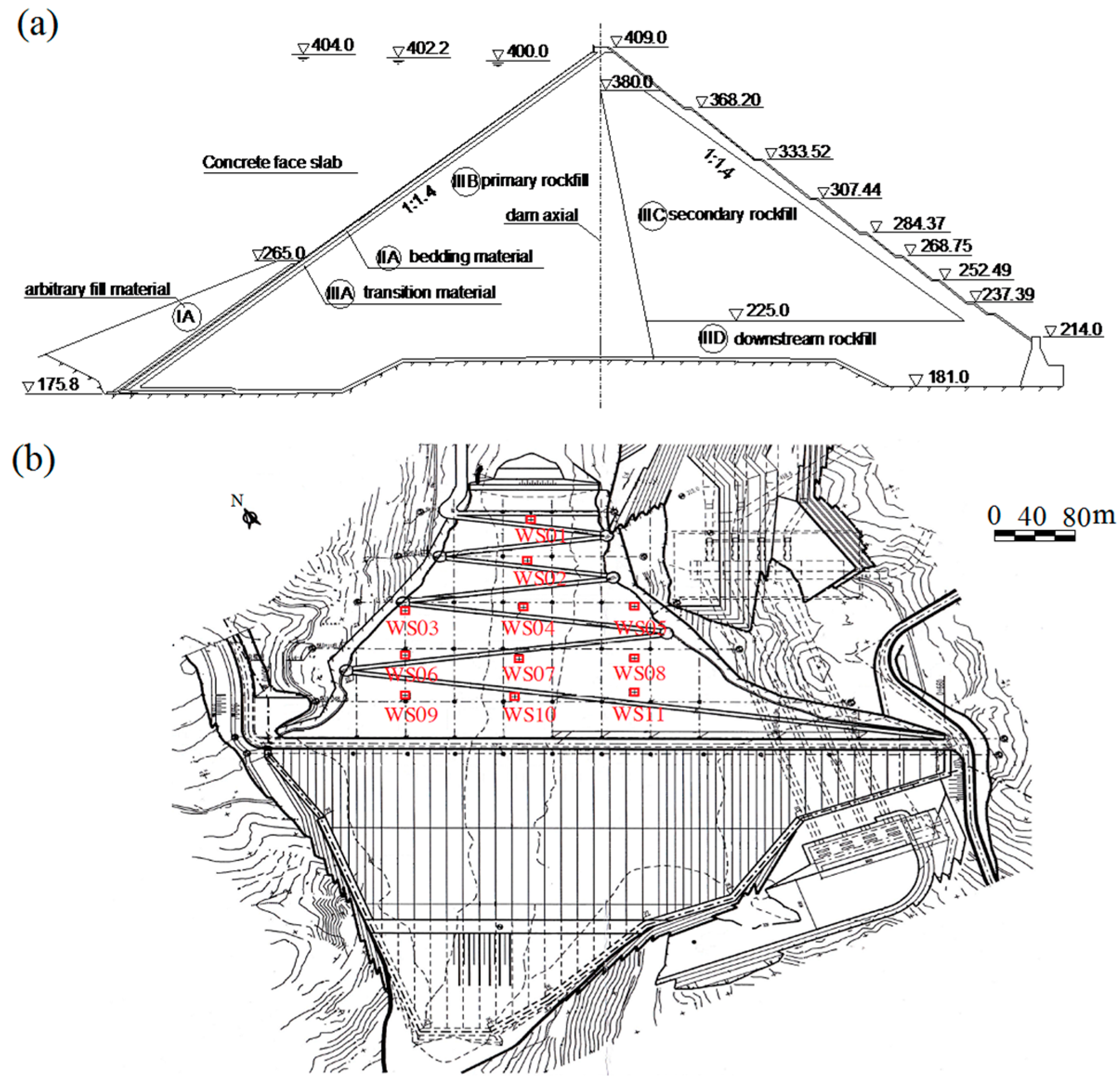
2. Study Area
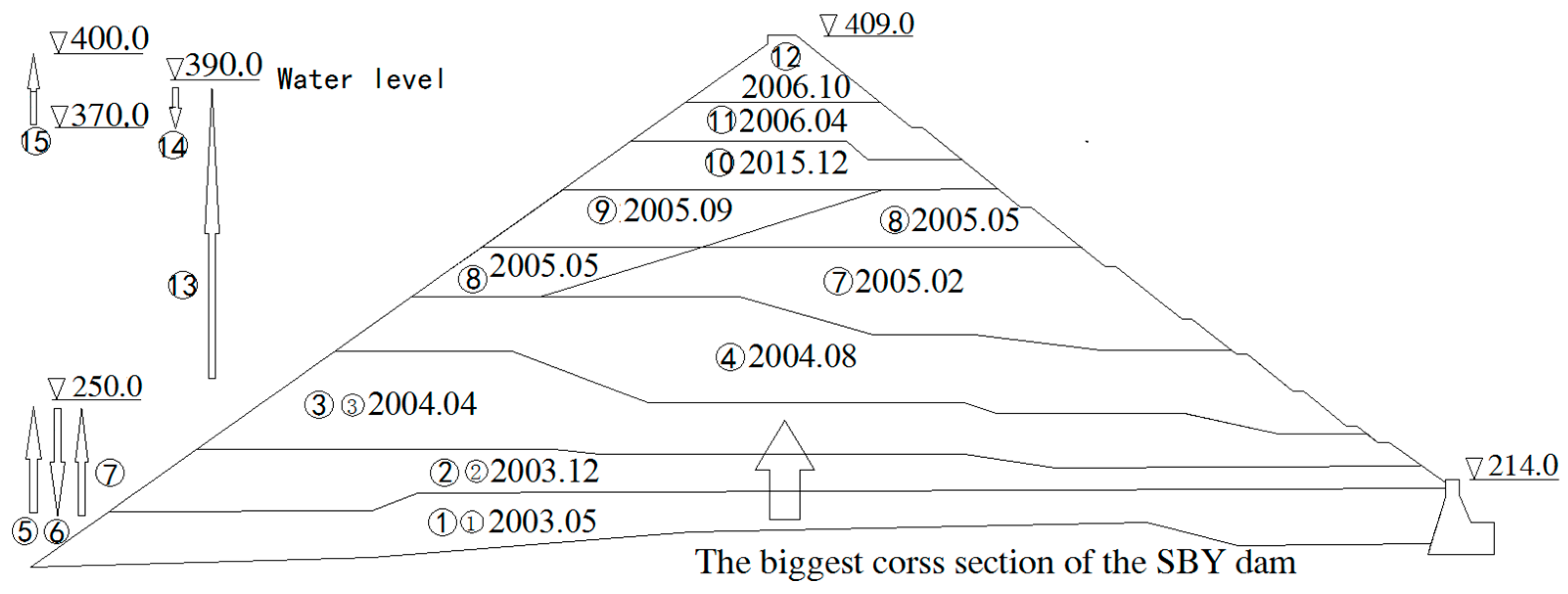
- Dam construction period (before October 2006).
- The first reservoir filling period (October 2006–September 2007, when the water level was between 205.06 m above sea level and 389.61 m).
- Operation period (after September 2007).
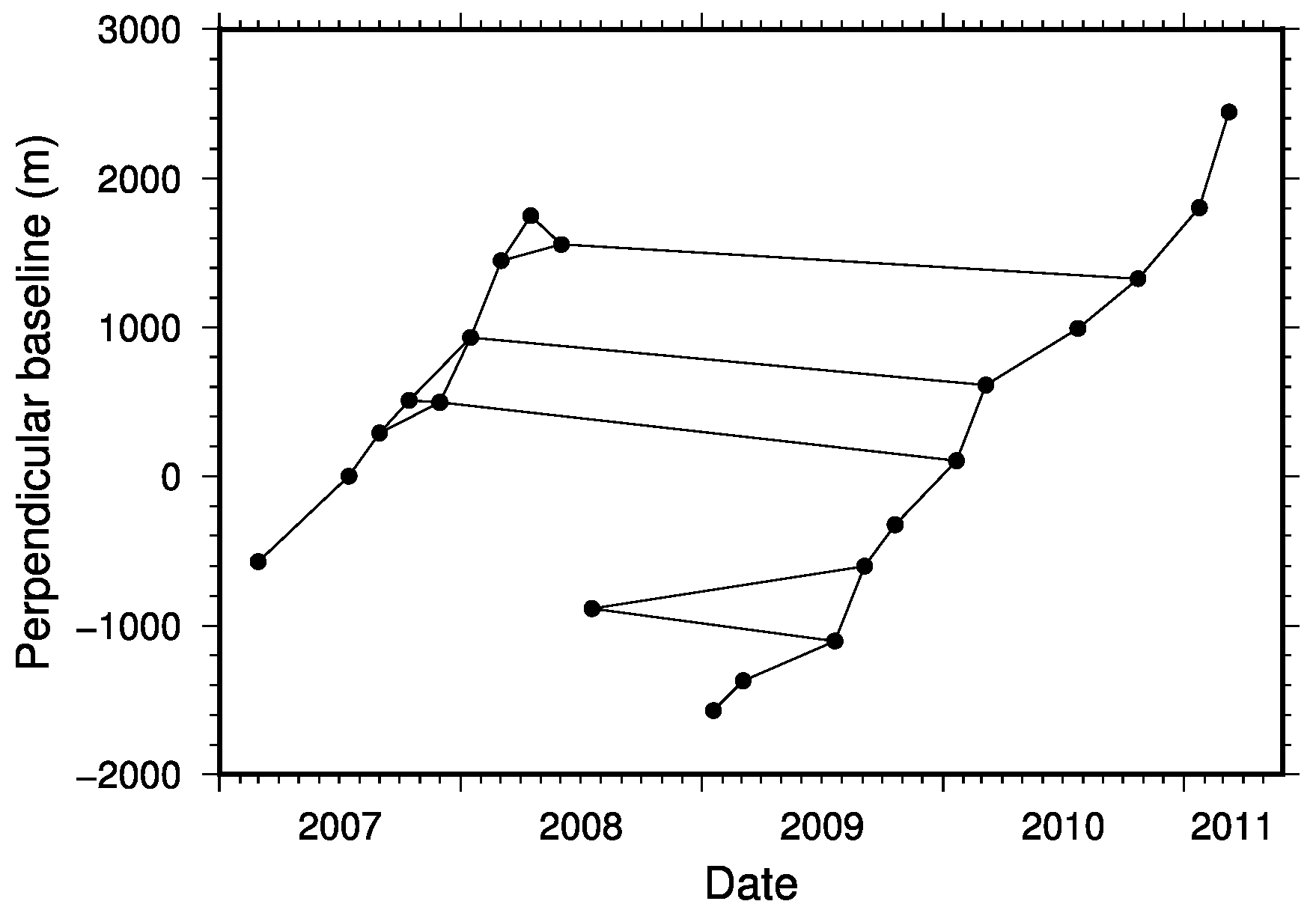
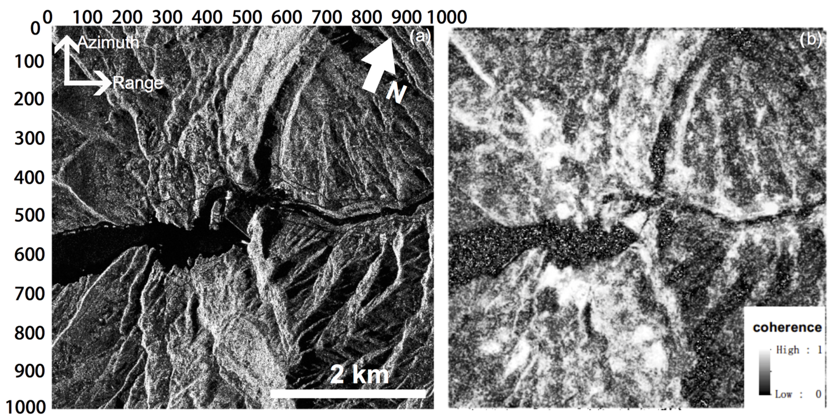
3. InSAR Data Analysis and Results
4. Mechanical Parameter Back-Analysis Using the FEM and InSAR Results
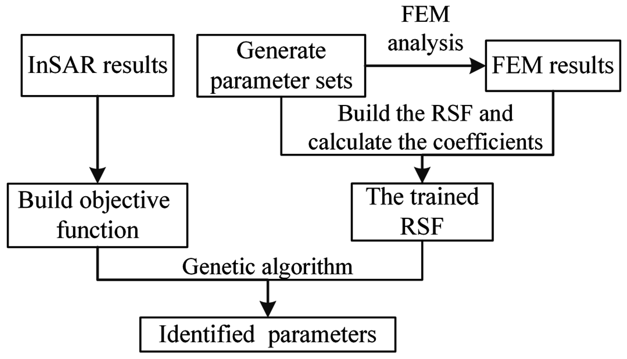
4.1. Mechanical Parameters Back-Analysis Method
- Build the objective function using the InSAR results, as Equation (2). Equation (2) presents the InSAR results of ith monitoring point.
- Perform the strain-stress analysis using the FEM (see Section 4.1.1) and the calculation of the RSM as defined in Section 4.1.2. Using the RSM, simulate the relationship between the parameter set and the displacement of each monitoring point.
- Find the optimal parameter set of the objective function using the modified genetic algorithm (GA) introduced in Section 4.1.3. The optimal parameter set is a combination of the material parameters that minimize the objective function. During the process of searching, these RSM are used to replace the FEM to calculate the fitness of all the measurement points.
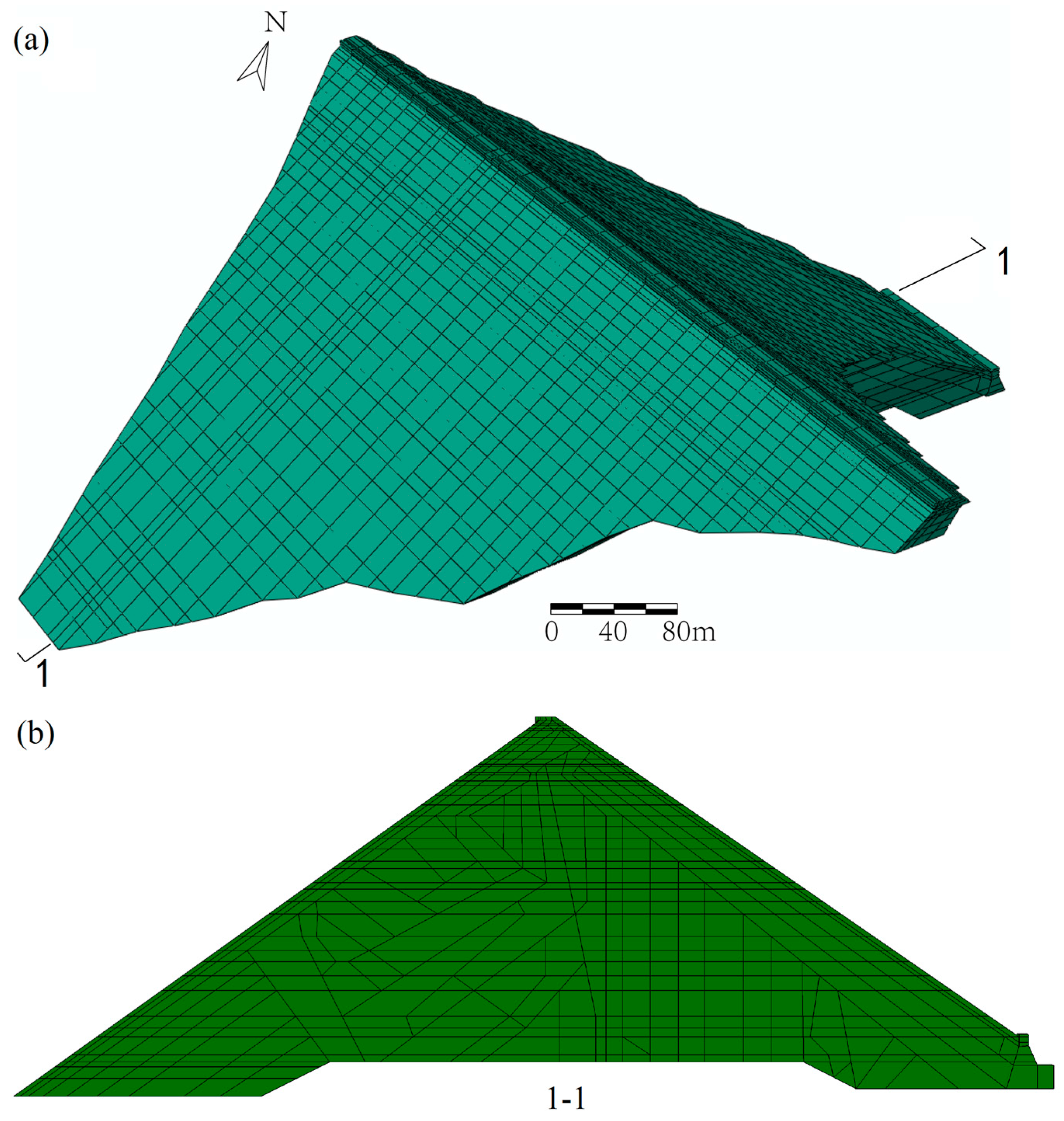
4.1.1. The FEM Model and the Constitutive Model
4.1.2. The Response Surface Method
4.1.3. The Modified Genetic Algorithm
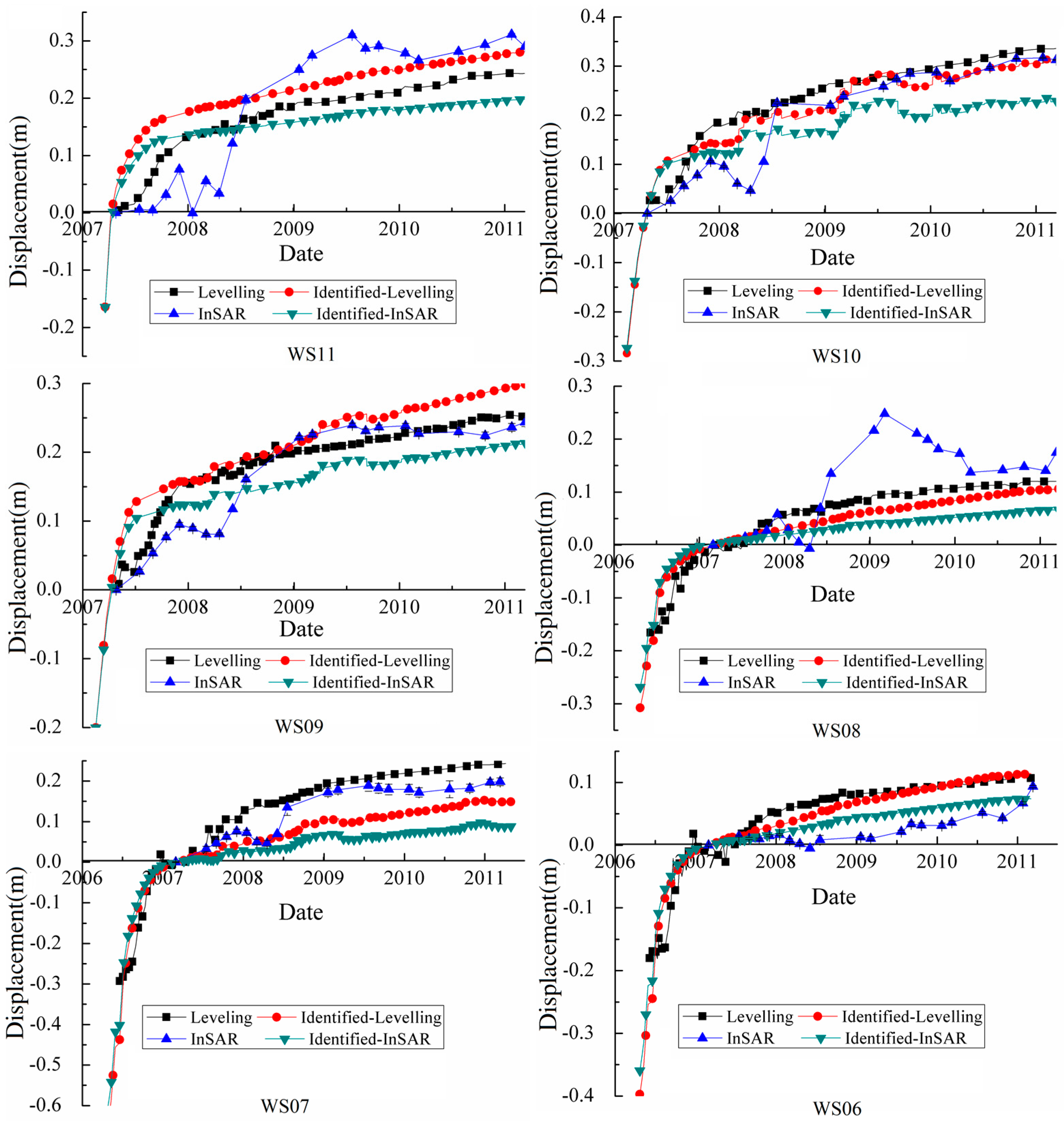
4.2. The Back-Analysis Results and the Argumentation
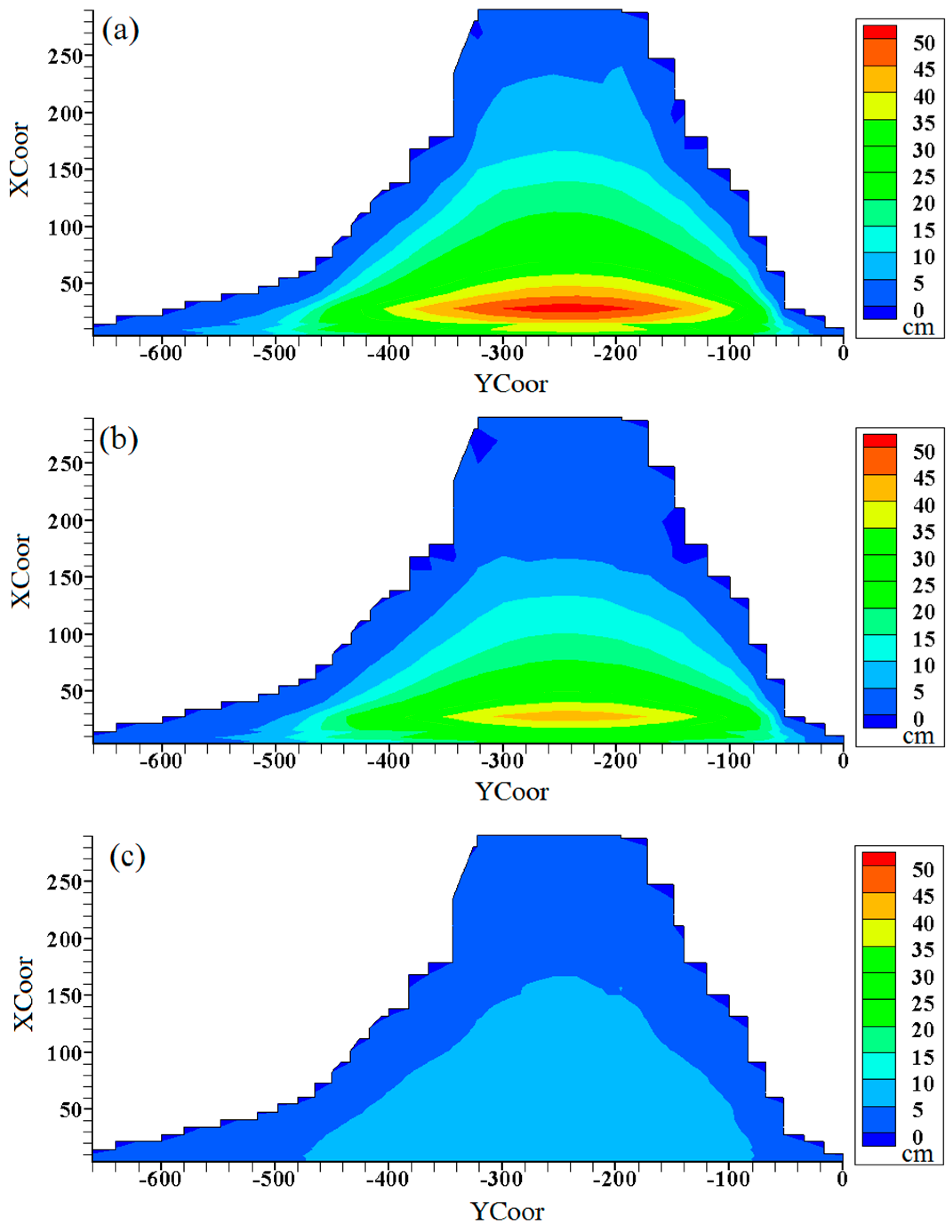
4.3. Settlement Prediction for the SBY Dam
5. Discussions
6. Conclusions
Acknowledgments
Author Contributions
Conflicts of Interest
References
- Wei, Z.; Xiaolin, C.; Chuangbing, Z.; Xinghong, L. Creep analysis of high concrete-faced rockfill dam. Int. J. Numer. Methods Biomed. Eng. 2010, 26, 1477–1492. [Google Scholar] [CrossRef]
- Hua, J.; Zhou, W.; Chang, X.; Zhou, C. Study of scale effect on stress and deformation of rockfill. Chin. J. Rock Mech. Eng. 2010, 2, 328–335. [Google Scholar]
- Wu, Y.; Yuan, H.; Zhang, B.; Zhang, Z.; Yu, Y. Displacement-based back-analysis of the model parameters of the nuozhadu high earth-rockfill dam. Sci. World J. 2014, 2014, 292450. [Google Scholar] [CrossRef] [PubMed]
- Li, S.J.; Zhang, J.; Liang, J.Q.; Sun, Z.X. Parameter inversion of nonlinear constitutive model of rockfill materials using observed deformations after dam construction. Rock Soil Mech. 2014, 35, 61–67. [Google Scholar]
- Jing, L. A review of techniques, advances and outstanding issues in numerical modelling for rock mechanics and rock engineering. Int. J. Rock Mech. Min. Sci. 2003, 40, 283–353. [Google Scholar] [CrossRef]
- Li, Z.; Li, J.; Zheng, S.; Wu, Q. Several measures for improving hydraulic overflow settlement gauge. Hydropower Autom. Dam Monit. 2010, 6, 31–33. [Google Scholar]
- Han, J.; Zhang, C. Experimental research on the installation of pipe-type settlement gauge in nuozhadu hydropower station. Water Power 2012, 38, 96–99. [Google Scholar]
- Liu, G.; Li, Z.; Li, X.; Wang, J. Experimental analysis of horizontal displacement monitoring device with long pipeline tensile. Hydropower Autom. Dam Monit. 2012, 4, 53–56. [Google Scholar]
- Yu, Y.; Zhang, B.; Yuan, H. An intelligent displacement back-analysis method for earth-rockfill dams. Comput. Geotech. 2007, 34, 423–434. [Google Scholar] [CrossRef]
- Zhao, H.-B.; Yin, S. Geomechanical parameters identification by particle swarm optimization and support vector machine. Appl. Math. Model. 2009, 33, 3997–4012. [Google Scholar] [CrossRef]
- Zheng, D.; Cheng, L.; Bao, T.; Lv, B. Integrated parameter inversion analysis method of a CFRD based on multi-output support vector machines and the clonal selection algorithm. Comput. Geotech. 2013, 47, 68–77. [Google Scholar] [CrossRef]
- Di Martire, D.; Iglesias, R.; Monells, D.; Centolanza, G.; Sica, S.; Ramondini, M.; Pagano, L.; Mallorquí, J.J.; Calcaterra, D. Comparison between differential SAR interferometry and ground measurements data in the displacement monitoring of the earth-dam of Conza della Campania (Italy). Remote Sens. Environ. 2014, 148, 58–69. [Google Scholar] [CrossRef]
- Wang, T.; Perissin, D.; Rocca, F.; Liao, M.-S. Three gorges dam stability monitoring with time-series InSAR image analysis. Sci. China Earth Sci. 2011, 54, 720–732. [Google Scholar] [CrossRef]
- Lazecký, M.; Perissin, D.; Zhi, W.; Ling, L.; Yu, Q. Observing dam’s movements with spaceborne SAR interferometry. In Engineering Geology for Society and Territory; Lollino, G., Manconi, A., Guzzetti, F., Culshaw, M., Bobrowsky, P., Luino, F., Eds.; Springer: Berlin/Heidelberg, Germany, 2015; Volume 5, pp. 131–136. [Google Scholar]
- Voege, M.; Frauenfelder, R.; Larsen, Y. Displacement monitoring at Svartevatn dam with interferometric SAR. In Proceedings of the 2012 IEEE International Geoscience and Remote Sensing Symposium (IGARSS), Munich, Germany, 22–27 July 2012; pp. 3895–3898.
- Zhou, W.; Li, S.; Zhou, Z.; Chang, X. Remote sensing of deformation of a high concrete-faced rockfill dam using InSAR: A study of the Shuibuya dam, China. Remote Sens. 2016, 8, 255. [Google Scholar] [CrossRef]
- Werner, C.; Wegmüller, U.; Strozzi, T.; Wiesmann, A. Gamma SAR and interferometric processing software. In Proceedings of the ERS-Envisat Symposium, Gothenburg, Sweden, 16–20 October 2000; p. 1620.
- Farr, T.G.; Rosen, P.A.; Caro, E.; Crippen, R.; Duren, R.; Hensley, S.; Kobrick, M.; Paller, M.; Rodriguez, E.; Roth, L.; et al. The shuttle radar topography mission. Rev. Geophys. 2007, 45, RG2004. [Google Scholar] [CrossRef]
- Eineder, M.; Hubig, M.; Milcke, B. Unwrapping large interferograms using the minimum cost flow algorithm. In Processdings of the 1998 Geoscience and Remote Sensing Symposium Proceedings, Seattle, WA, USA, 6–10 July 1998; pp. 83–87.
- Hanssen, R.F. Radar Interferometry: Data Interpretation and Error Analysis; Kluwer Academic Plublishers: Dordrecht, The Netherlands, 2001. [Google Scholar]
- Ferretti, A.; Prati, C.; Rocca, F. Permanent scatterers in SAR interferometry. IEEE Trans. Geosci. Remote Sens. 2001, 39, 8–20. [Google Scholar] [CrossRef]
- Berardino, P.; Fornaro, G.; Lanari, R.; Sansosti, E. A new algorithm for surface deformation monitoring based on small baseline differential SAR interferograms. IEEE Trans. Geosci. Remote Sens. 2002, 40, 2375–2383. [Google Scholar] [CrossRef]
- Hooper, A.; Segall, P.; Zebker, H. Persistent scatterer interferometric synthetic aperture radar for crustal deformation analysis, with application to Volcán Alcedo, Galápagos. J. Geophys. Res. 2007, 112, B07407. [Google Scholar] [CrossRef]
- Doin, M.-P.; Guillaso, S.; Jolivet, R.; Lasserre, C.; Lodge, F.; Ducret, G.; Grandin, R. Presentation of the small-baseline NSBAS processing chain on a case example: The Etna deformation monitoring from 2003 to 2010 using Envisat data. In Proceedings of the Fringe Symposium, Frascati, Italy, 19–23 September 2011; pp. 303–304.
- Ferretti, A.; Fumagalli, A.; Novali, F.; Prati, C.; Rocca, F.; Rucci, A. A new algorithm for processing interferometric data-stacks: Squeesar. IEEE Trans. Geosci. Remote Sens. 2011, 49, 1–11. [Google Scholar] [CrossRef]
- Li, Z.; Fielding, E.J.; Cross, P. Integration of InSAR time-series analysis and water-vapor correction for mapping postseismic motion after the 2003 Bam (Iran) earthquake. IEEE Trans. Geosci. Remote Sens. 2009, 47, 3220–3230. [Google Scholar]
- Zhang, L.; Ding, X.; Lu, Z. Ground settlement monitoring based on temporarily coherent points between two SAR acquisitions. ISPRS J. Photogramm. Remote Sens. 2011, 66, 146–152. [Google Scholar] [CrossRef]
- Sowter, A.; Bateson, L.; Strange, P.; Ambrose, K.; Syafiudin, M.F. DInSAR estimation of land motion using intermittent coherence with application to the South Derbyshire and Leicestershire coalfields. Remote Sens. Lett. 2013, 4, 979–987. [Google Scholar] [CrossRef]
- Li, Z.; Fielding, E.J.; Cross, P.; Muller, J.-P. Interferometric synthetic aperture radar atmospheric correction: GPS topography-dependent turbulence model. J. Geophys. Res. Solid Earth 2006, 111, B02404. [Google Scholar] [CrossRef]
- Williams, S.; Bock, Y.; Fang, P. Integrated satellite interferometry: Tropospheric noise, GPS estimates and implications for interferometric synthetic aperture radar products. J. Geophys. Res. Solid Earth 1998, 103, 27051–27067. [Google Scholar] [CrossRef]
- Hammond, W.C.; Blewitt, G.; Li, Z.; Plag, H.P.; Kreemer, C. Contemporary uplift of the Sierra Nevada, western United States, from GPS and InSAR measurements. Geology 2012, 40, 667–670. [Google Scholar] [CrossRef]
- Zienkiewicz, O.C.; Taylor, R.L.; Zienkiewicz, O.C.; Taylor, R.L. The Finite Element Method; McGraw-Hill: London, UK, 1977; Volume 3. [Google Scholar]
- Duncan, J.M.; Chang, C.-Y. Nonlinear analysis of stress and strain in soils. J. Soil Mech. Found. Div. 1970, 96, 1629–1653. [Google Scholar]
- Duncan, J.M.; Wong, K.S.; Mabry, P. Strength, stress–strain and bulk modulus parameters for finite element analyses of stresses and movements in soil masses. In Geotechnical Engineering; University of California: Berkeley, CA, USA, 1980. [Google Scholar]
- Wang, G.-Q.; Yu, T.; Li, Y.-H.; Li, G.-Y. Creep deformation of 300 m-high earth core rockfill dam. Chin. J. Geotech. Eng. 2014, 36, 140–145. [Google Scholar]
- Holland, J.H. Adaptation in Natural and Artificial Systems. An Introductory Analysis with Application to Biology, Control, and Artificial Intelligence; University of Michigan Press: Ann Arbor, MI, USA, 1975. [Google Scholar]


| Parameters | K1 | n1 | Kb1 | m1 | K2 | n2 | Kb2 | m2 | a | b (%) | mc | β (%) | d (%) |
|---|---|---|---|---|---|---|---|---|---|---|---|---|---|
| Experimental | 1100 | 0.35 | 600 | 0.1 | 850 | 0.25 | 400 | 0.05 | 0.009 | 0.0098 | 1.1338 | 0.64 | 0.21 |
| Identified 1# | 876 | 0.284 | 512 | 0.115 | 967 | 0.203 | 320 | 0.0579 | 0.00069 | 0.0113 | 1.334 | 0.77 | 0.168 |
| Identified 2# | 958 | 0.31 | 550 | 0.10 | 816 | 0.225 | 375 | 0.05 | 0.0007 | 0.0088 | 0.907 | 0.512 | 0.17 |
© 2016 by the authors; licensee MDPI, Basel, Switzerland. This article is an open access article distributed under the terms and conditions of the Creative Commons Attribution (CC-BY) license (http://creativecommons.org/licenses/by/4.0/).
Share and Cite
Zhou, W.; Li, S.; Zhou, Z.; Chang, X. InSAR Observation and Numerical Modeling of the Earth-Dam Displacement of Shuibuya Dam (China). Remote Sens. 2016, 8, 877. https://doi.org/10.3390/rs8100877
Zhou W, Li S, Zhou Z, Chang X. InSAR Observation and Numerical Modeling of the Earth-Dam Displacement of Shuibuya Dam (China). Remote Sensing. 2016; 8(10):877. https://doi.org/10.3390/rs8100877
Chicago/Turabian StyleZhou, Wei, Shaolin Li, Zhiwei Zhou, and Xiaolin Chang. 2016. "InSAR Observation and Numerical Modeling of the Earth-Dam Displacement of Shuibuya Dam (China)" Remote Sensing 8, no. 10: 877. https://doi.org/10.3390/rs8100877