A Multi-Resolution Blending Considering Changed Regions for Orthoimage Mosaicking

Abstract

Blending processing based on seamlines in image mosaicking is a procedure designed to obtain a smooth transition between images along seamlines and make seams invisible in the final mosaic. However, for high-resolution aerial orthoimages in urban areas, factors such as projection differences, moving objects, and radiometric differences in overlapping areas may result in ghosting and artifacts or visible shifts in the final mosaic. Such a mosaic is not a true reflection of the earth’s surface and may have a negative impact on image interpretation. Therefore, this paper presents a multi-resolution blending method considering changed regions to improve mosaic image quality. The method utilizes the region change rate (RCR) to distinguish changed regions from unchanged regions in overlapping areas. The RCR of each region is computed using image segmentation and change detection methods. Then, a mask image is generated considering changed regions, and Gaussian and Laplacian pyramids are constructed. Finally, a multi-resolution reconstruction is performed to obtain the final mosaic. Experimental results from digital aerial orthoimages in urban areas are provided to verify this method for blending processing based on seamlines in mosaicking. Comparisons with other methods further demonstrate the potential of the presented method, as shown in a detailed comparison in three typical cases of the seamline passing by buildings, the seamline passing through buildings, and the seamline passing through areas with large radiometric differences.

1. Introduction

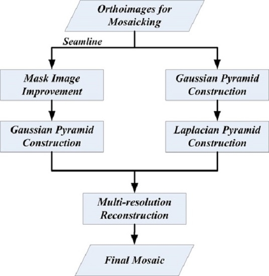
Orthoimage mosaicking is the process of combining multiple orthorectrified images into a single seamless composite image. It is also a necessary process for covering a large geographic region in many applications, e.g., environmental monitoring, disaster management, and the construction of digital cities or smart cities [1,2]. When mosaicking orthoimages, the seam-based method is the most popular method. Generally, the seam-based method will define seamlines in overlapping regions. Then, in mosaicking, each pixel in the final result is represented entirely by one orthoimage based on which side of the seamline it lies on. Finally, a blending processing, also called feathering, based on seamlines is performed to make the seam invisible in the final mosaic. This paper focuses on the blending processing in mosaicking, i.e., a procedure to obtain a smooth transition between images along seamlines.

In orthoimages, objects above or below the digital terrain model (DTM) used for orthorectification will be geometrically displaced due to perspective imaging from different view angles. There are often obvious projection differences in overlapping areas and different facets of an object, e.g., a building, may appear in different images, especially for high-resolution aerial orthoimages in urban areas. Those phenomena are more obvious the higher the objects are [1]. When such phenomena occur, there are obvious misalignments between orthoimages. Moving objects, e.g., cars, are also shown as obvious misalignments between orthoimages. Thus, in the blending processing, it becomes more difficult to make the seam invisible in the mosaic. Radiometric differences due to the different viewing angles or illumination conditions between orthoimages also bring difficulties and may cause visible shifts in brightness or color.

Generally, in blending processing, mosaic image $I$ is a weighted combination of the input images $I_1$ and $I_2$ over the overlapping areas. The weighting coefficients vary as a function of the distance from the seamline. Milgram (1975) defined a linear ramp to pixel values on either side of the seamline as the weighting function to obtain equal values at the seamline itself [3]. Li et al. (2015) improved the weighting function, and presented a cosine distance weighted blending method for high spatial resolution remote sensing images in which the weight calculation algorithm is based on the cosine distance [4]. Burt and Adelson (1983) presented a pyramid blending approach where images were decomposed into a set of band-pass filtered component images. Then, different frequency bands were combined with different weighting coefficients and the component images in each spatial frequency band are assembled into a corresponding band-pass mosaic. Finally, these band-pass mosaic images are summed to obtain the desired image mosaic [5,6]. Brown and Lowe (2007) also used the same pyramid blending approach in [5] for the panoramic image stitching [7]. Shao et al. (2012) improved the pyramid blending approach in [5] for asymmetrically informative biological images during microscope image stitching. They optimized the blending coefficients based on the constraint of the information imbalance between the earlier- and later-acquired images [8]. Uyttendaele et al. (2001) presented a feathering method, which used averaging and interpolation functions to eliminate ghosting and reduce intensity differences [9]. Zhu and Qian (2002) presented a hard correction method to remove a possible seam. It first obtained the mosaic image directly based on seamlines without any blending processing in overlapping areas. Then, the average difference within a certain extent of the two sides of the seamline was computed and corrected within a certain extent of the two sides of the seamline [10]. Pérez et al. (2003) proposed a framework for image editing, i.e., object insertion, in the gradient domain. The object is cut from an image and inserted into a new background image. The insertion is performed by optimizing over the gradients of the inserted object [11]. Levin et al. (2004) and Zomet et al. (2006) proposed a gradient-domain image stitching method. The method introduced several formal cost functions for the evaluation of the stitching quality in the gradient domain and defined the mosaic image as their optimum in the overlapping areas [12,13]. Jia and Tang (2008) proposed an image stitching approach by image deformation. The approach propagated the deformation into the target image smoothly and both structure deformation and colour correction were simultaneously achieved within the same framework operating in the image gradient domain [14].

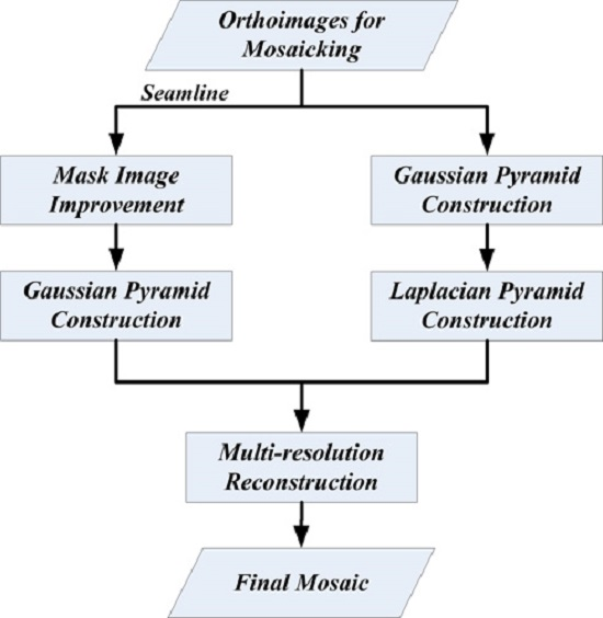
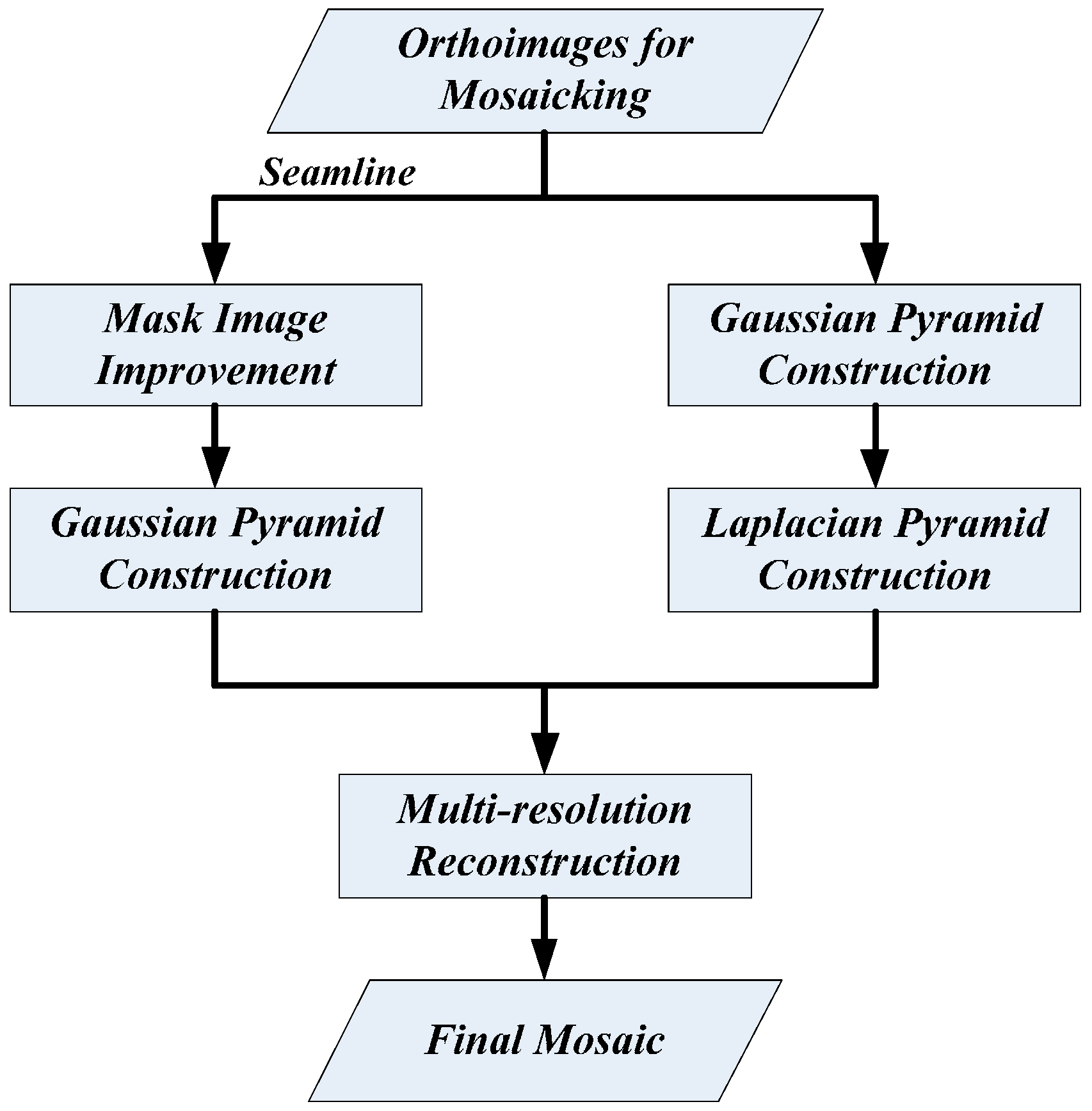
Most of these methods deal with natural images and focus on the visual effect. However, these methods still do not fully meet the requirements for remote sensed images in earth observation. In earth observation, orthoimages are orthorectifed remote sensed images with precise geocoding and should reflect the earth’s surface as accurately as possible. The visual effect is of secondary importance. A mosaic of orthoimages is no exception. Unlike natural images, misalignments in orthoimages generally appear in regions with objects such as buildings, bridges, and moving cars. For high-resolution aerial orthoimages in urban areas, such misalignments are usually large and different facades of objects may appear in different images. If only considering the visual effect, ghosting and artifacts may be created in the mosaic image that are not only not a true reflection of earth’s surface but also harmful in image interpretation. Thus, these regions should be treated differently from other regions to ensure the mosaic image can reflect the earth’s surface as accurately as possible. Therefore, in this paper, a multi-resolution blending method considering changed regions for orthoimage mosaicking is presented. In this method, regions with obvious projection differences (e.g., buildings) or moving objects (e.g., cars) are considered as changed regions. In the blending procedure, changed regions and unchanged regions are treated differently: changed regions will be blended within a limited width or blending will be avoided, and unchanged regions will be blended in the set blending width to achieve a smooth transition.

2. Methods

A flowchart of the presented method is shown in Figure 1. Image segmentation and change detection are used to determine changed regions, i.e., regions with obvious projection differences or moving objects in orthoimages, and then the generation of the mask image is improved to enlarge the transition zone width in unchanged regions. The Gaussian pyramid construction, Laplacian pyramid construction, and multi-resolution reconstruction are similar to the pyramid blending method in [5]. By doing so, a smooth transition can be obtained in unchanged regions, while changed regions are blended in a relatively narrow transition zone and ghosting and artifacts can be avoided.

2.1. Mask Image Improvement

Mask image improvement is different from mask image generation in the pyramid blending method in [5]. This paper enlarges the transition zone width by adding a smooth filter to the mask image. To prevent the mosaic image from affecting image interpretation, changed regions and unchanged regions are treated differently. Regions with obvious projection differences or moving objects are considered as changed regions, e.g., buildings, bridges, and moving cars in orthoimages. When adding a smooth filter on the mask image, values of pixels in changed regions remain unchanged. Changed regions are determined by the region change rate (RCR), which is the change rate of the segmented region and is calculated based on the percentage of changed pixels in the segmented region. The main steps of mask image improvement is as follows: (1) deriving differences in overlaps; (2) determining changed regions; and (3) generating mask image.

2.1.1. Deriving Differences in Overlaps

In this paper, texture similarity is used to derive differences in overlaps. Overlaps can be determined by the geocoding information. The texture similarity of pixel $(i,j)$ in the overlap between adjacent images is calculated as the following equation:

$$Cost(i,j)=INT(255\times (1-\rho )/2.0)$$

(1)

where $\rho$ is the normalized cross correlation (NCC) for pixel $(i,j)$ in the overlap and it is computed using a subimage centered around pixel $(i,j)$; and $INT$ is integer rounding operations. Let $A$, $B$ be the left image and right image (two arbitrary images captured in different times with overlap) in the overlap, respectively. The detailed equation of $\rho$ for pixel $(i,j)$ in the overlap is as follows:

$$\rho =\frac{{\displaystyle \sum _{i=1}^M{\displaystyle \sum _{j=1}^N(A(i,j)-\overline{A})}}\cdot (B(i,j)-\overline{B})}{\sqrt{{\displaystyle \sum _{i=1}^M{\displaystyle \sum _{j=1}^N{(A(i,j)-\overline{A})}^2}}\cdot {\displaystyle \sum _{i=1}^M{\displaystyle \sum _{j=1}^N{(B(i,j)-\overline{B})}^2}}}}$$

(2)

where $\overline{A}=\frac{1}{M\times N}{\displaystyle \sum _{i=1}^M{\displaystyle \sum _{j=1}^{N}A(i,j)}}$, $A(i,j)$ is the value of pixel $(i,j)$ in left image; and $\overline{B}=\frac{1}{M\times N}{\displaystyle \sum _{i=1}^M{\displaystyle \sum _{j=1}^{N}B(i,j)}}$, $B(i,j)$ is the value of pixel $(i,j)$ in right image [15]. Because $\rho$ has a range of [−1.0, 1.0], $Cost(i,j)$ has a range of [0, 255].

2.1.2. Determining Changed Regions

Changed regions are determined by the RCR. To calculate the RCR for segmented regions, changed pixels in overlapping areas should be obtained first based on change detection. Change detection is the process of identifying differences in the state of an object or phenomenon by observing it at different times. In this paper, differences in overlaps are derived by texture similarity described in Section 2.1.1. The procedure yields a difference distribution for each band. In such a distribution, pixels exhibiting changes are found in the tails of the distribution whereas pixels exhibiting no changes tend to be grouped around the mean. A critical element of the image differencing method is deciding where to place the threshold boundaries between changed and unchanged pixels displayed in the histogram [16,17].

Then, the changed and unchanged pixels are distinguished by the following equation:

$$\left|Cost(i,j)-m\right|\ge T_d\sigma$$

(3)

where $m$ and $\sigma$ are the mean and standard deviation of the texture similarity image, respectively, and $T_d$ is the given threshold that distinguishes changed and unchanged pixels. Pixels in the overlap that satisfy Equation (3) are considered changed pixels and other pixels are unchanged pixels.

At this time, the RCR can be computed by combining the segmented regions and the changed pixels in the overlap. It is the percentage of changed pixels in the segmented region and defined by the following equation:

$$RCR=\frac{Nu{m}_C}{Num}$$

(4)

where $RCR$ is the change rate of the current segmented region, $Nu{m}_C$ is the number of changed pixels in the segmented region, and $Num$ is the number of pixels in the segmented region.

As to image segmentation, we use the mean shift (MS) algorithm in this paper and overlaps in the left and right images are segmented separately. MS is an algorithm of nonparametric density gradient estimation. Its application domains include clustering in computer vision and image processing [18,19,20]. Let data be a finite set $S$ embedded in the n-dimensional Euclidean space $X$. Let $K$ be a kernel, and weight be a weight function. The sample mean with kernel $K$ at $x\in X$ is defined as

$$m(x)=\frac{{\displaystyle \sum _{s\in S}K(s-x)w\mathrm{eight}(s)s}}{{\displaystyle \sum _{s\in S}K(s-x)w\mathrm{eight}(s)}}$$

(5)

Let $T\subset X$ be a finite set. The evolution of $T$ in the form of iterations $T\leftarrow m(T)$ with $m(T)=\{m(t);t\in T\}$ is called an MS algorithm. For each $t\in T$, there is a sequence $t,m(t),m(m(t)),\dots ,$ which is called the trajectory of $t$. The weight $w\mathrm{eight}(s)$ can either be fixed throughout the process or re-evaluated after each iteration. It may also be a function of the current $T$. The algorithm halts when it reaches a fixed point, i.e., when $m(T)$ converges [19]. Among the various implementations of MS, the Edge Detection and Image SegmentatiON (EDISON) library in C++ was used to complete the image segmentation in this paper [21].

After calculating the RCR for each segmented region, a threshold of the RCR, i.e., changed region threshold $TRate$, is set to determine whether a region belongs to a changed region. If the RCR of a region is larger than $TRate$, it is a changed region; otherwise it is an unchanged region. The determination of changed regions by $TRate$ is performed in the overlap of the left and right images independently. Assuming $R1$ and $R2$ are the changed regions of the left and right images in the overlap, respectively, the final changed regions in the overlap, $R$, are the union regions of $R1$ and $R2$, i.e., $R=R1\cup R2$.

2.1.3. Generating Mask Image

Mask image $M$ is generated according to the seamline and the determined changed regions in the overlap. It is used to enlarge the transition zone width when pyramid blending.

First is the construction of the initial mask image. A same-size 8-bit image is created with the overlap of the left and right images as the initial mask image. In the initial mask image, pixels on the left side of the seamline are assigned a value of 0 and the other pixels are assigned a value of 255.

Then, a smooth filter is added to the initial mask image. Based on the changed regions $R$, smoothing is carried out selectively. Changed regions and unchanged regions are treated differently. In smoothing, values of pixels in changed regions remain unchanged. Both a Gaussian filter and a mean smoothing filter can be selected as the smooth filter. The size of the smooth filter can be set by the user according to the requirements of blending procedure.

2.2. Gaussian Pyramid Construction

Gaussian pyramid is built for left image $A$, right image $B$, and mask image $M$, respectively. It is a set of low-pass filtered images. Taking the left image $A$ as an example, the Gaussian pyramid construction is described as follows [5].

The origin left image $A$ is the level 0 image of the Gaussian pyramid. Then, according to Equation (6), other level images of the Gaussian pyramid can be computed by a low-pass window mask $w$ from the lower level image iteratively. By doing so, the Gaussian pyramid of the left image $A$, i.e., $G{S}_A$, can be obtained. The image size of the upper level image in the Gaussian pyramid is half of the closest lower level image. The detailed pyramid computation equation is as follows:

$$G{S}^l(i,j)={\displaystyle \sum _{m=-2}^2{\displaystyle \sum _{n=-2}^2{w}_{m,n}G{S}^{l-1}(2i+m,2j+n)}}$$

(6)

where $0<l\le N$, $l$ is an integer; $G{S}^l(i,j)$ is the value of pixel $(i,j)$ in level $l$ image of the Gaussian pyramid; $N$ is the number of levels of the Gaussian pyramid, and in this paper, $N=3$; $w$ is a low-pass window mask with a size of 5 by 5; and $w_{m,n}$ is the value of a specific element in the window mask ($-2\le m,n\le 2$, $m$, $n$ are integers). The detailed definition of $w$ is as follows:

$$w=\frac{1}{256}\left[\begin{array}{ccccc}1& 4& 6& 4& 1\\ 4& 16& 24& 16& 4\\ 6& 24& 36& 24& 6\\ 4& 16& 24& 16& 4\\ 1& 4& 6& 4& 1\end{array}\right]$$

(7)

For right image $B$ and mask image $M$, their Gaussian pyramid $G{S}_B$ and $G{S}_M$ are built in the same way as the left image $A$.

2.3. Laplacian Pyramid Construction

Laplacian pyramid is built for left image $A$ and right image $B$, respectively. Their Laplacian pyramids $L{P}_A$ and $L{P}_B$ are built in the same way. Taking the left image $A$ as an example, the Laplacian pyramid construction is described as follows [5].

According to Equation (8), each Gaussian pyramid level image $G{S}^l(i,j)$ ($0<l\le N$, $l$ is an integer) is interpolated to obtain $G{S}^{l\prime }(i,j)$. $G{S}^{l\prime }(i,j)$ is expanded to 2 times the size of $G{S}^l(i,j)$. $G{S}^{l\prime }(i,j)$ is the same size as $G{S}^{l-1}(i,j)$.

$$G{S}^{l\prime }(i,j)=EXPAND[G{S}^l]=4{\displaystyle \sum _{m=-2}^2{\displaystyle \sum _{n=-2}^2{w}_{m,n}G{S}^l(\frac{i+m}{2},\frac{j+n}{2})}}$$

(8)

In the computation process, the corresponding pixels are computed only when $\frac{i+m}{2}$ and $\frac{j+n}{2}$ are both integers and $EXPAND$ is the interpolation operation. Then, the level $l-1$ image of the Laplacian pyramid can be computed by the following equation ($0<l\le N$, $l$ is an integer):

$$L{P}^{l-1}(i,j)=G{S}^{l-1}(i,j)-G{S}^{l\prime }(i,j)$$

(9)

After each level image of the Laplacian pyramid is computed, the Laplacian pyramid for the left image $A$, i.e., $L{P}_A$, can be obtained.

2.4. Multi-Resolution Reconstruction

A multi-resolution reconstruction is the final step of the presented multi-resolution blending procedure to obtain the mosaic image. It combines the Laplacian pyramid images of the left and right images in the overlap using the Gaussian pyramid of the mask image $M$ as the weighting factor to obtain the stitching Laplacian pyramid image [5]. According to Equation (10), the Laplacian pyramid images of left image $A$ and right image $B$, i.e., $L{P}_A^l$ and $L{P}_B^l$, are combined level by level using the Gaussian pyramid of the mask image $M$ as the weighting factor to obtain the stitching Laplacian pyramid image $LP$.

$$L{P}^l=\left\{\left[255-G{S}_M^l(i,j)\right]\cdot L{P}_A^l(i,j)+G{S}_M^l(i,j)L{P}_B^l(i,j)\right\}/255$$

(10)

where $0\le l<N$ and $l$ is an integer. Then, the final mosaic image after multi-resolution blending can be reconstructed level by level based on the following equation:

$$\{\begin{array}{c}GS{R}^N=L{P}^N\\ GS{R}^{l-1}=L{P}^{l-1}+EXPAND(GS{R}^l)\end{array}$$

(11)

In Equation (11), $0<l\le N$, and $l$ is an integer; the definition of $EXPAND$ is same as in Equation (8). According to Equation (11), the reconstruction is carried out level by level until $GS{R}^0$ is obtained. $GS{R}^0$ is the final mosaic image after multi-resolution blending.

3. Results

The described algorithm above has been implemented in C++. The EDISON library is used for image segmentation and the Geospatial Data Abstraction Library (GDAL) is used to read and write image files. A number of digital aerial orthoimages have been employed to test the proposed algorithm, and two data sets are presented. In experiments on the two presented data sets, the MS segmentation parameters $(h_s,h_r,M)$ are set as (6, 5, 20), where $(h_s,h_r)$ are the bandwidth parameters and $M$ is the least significant feature size. The threshold to distinguish changed and unchanged pixels $T_d$ is set to 1.0. The threshold of RCR, $TRate$, is set to 0.2.

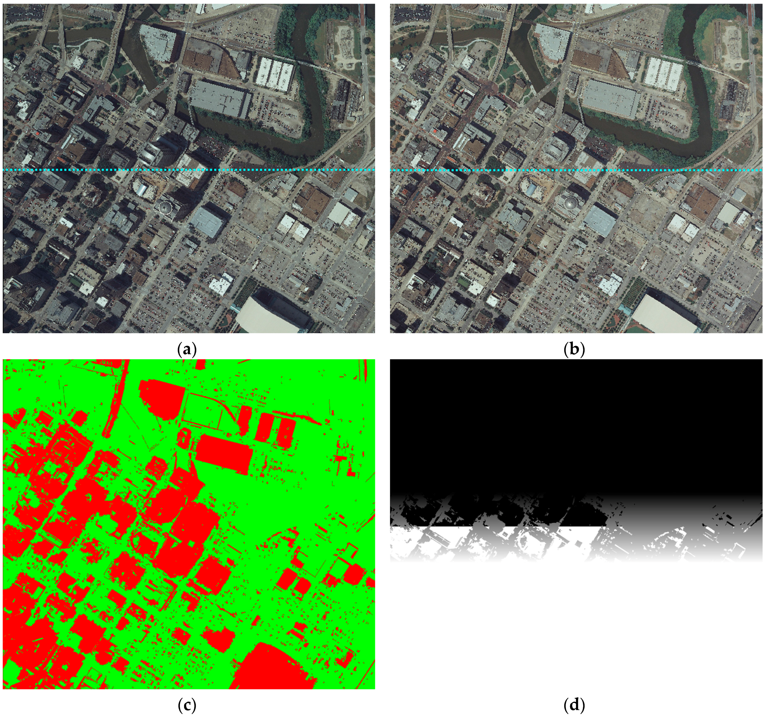
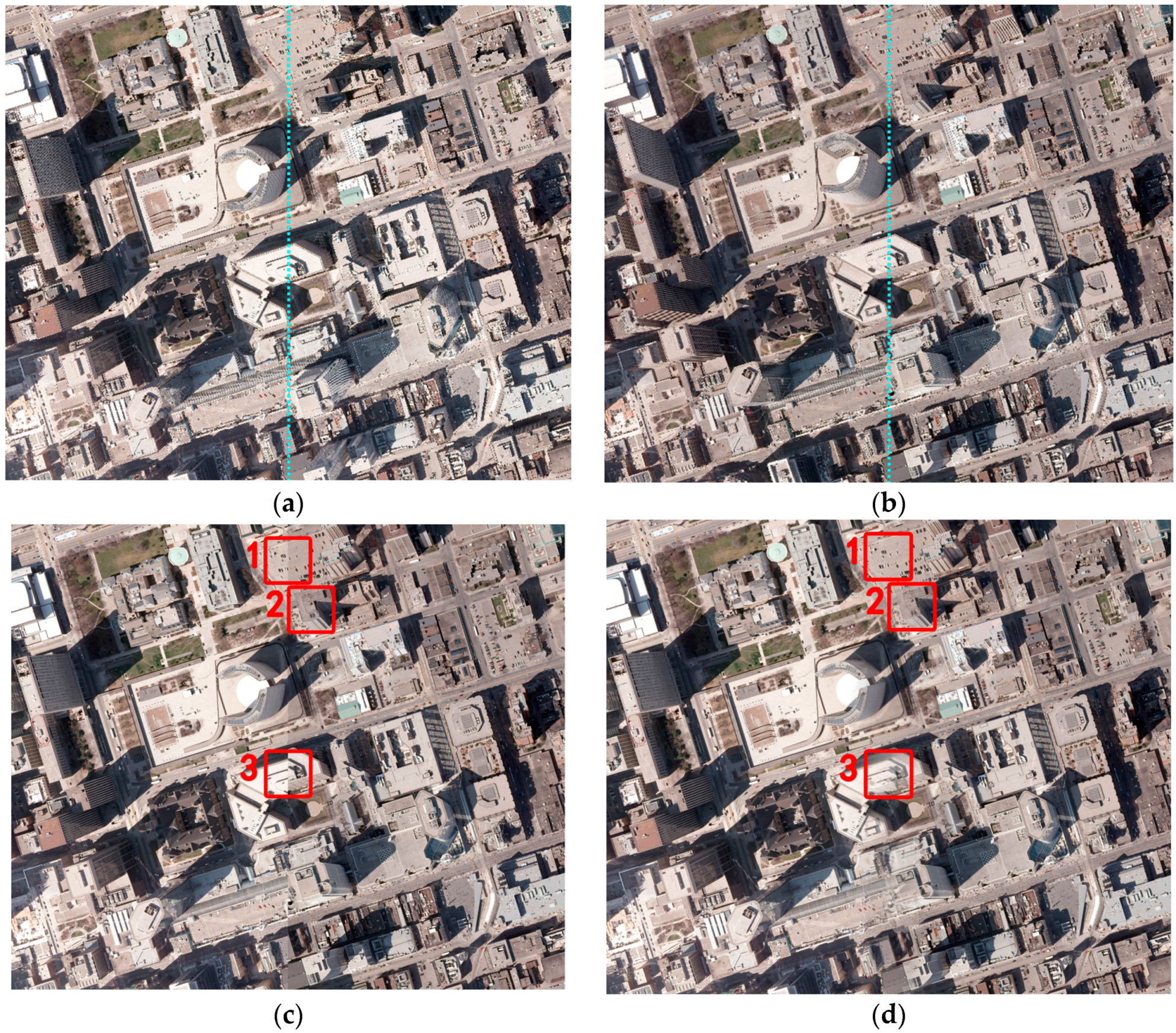
The image size of data set 1 is approximately 2000 by 1800 pixels. The performance of the presented method is demonstrated in Figure 2 and Figure 3. In Figure 2 and Figure 3, comparisons with the direct mosaic, the linear ramp weighting method [3], the cosine distance weighted blending method [4], and the pyramid blending method [5] are also presented. In these experiments, the blending width in the linear ramp weighting method and the cosine distance weighted blending method is 400 pixels, and there are 200 pixels on each side of the seamline. The size of the smooth filter to generate the mask image in the presented method is also 400 pixels. The left and right images overlapping seamlines (dotted line) are shown in Figure 2a,b, respectively. To simplify the problem, the seamline is considered a straight line in the experiments. 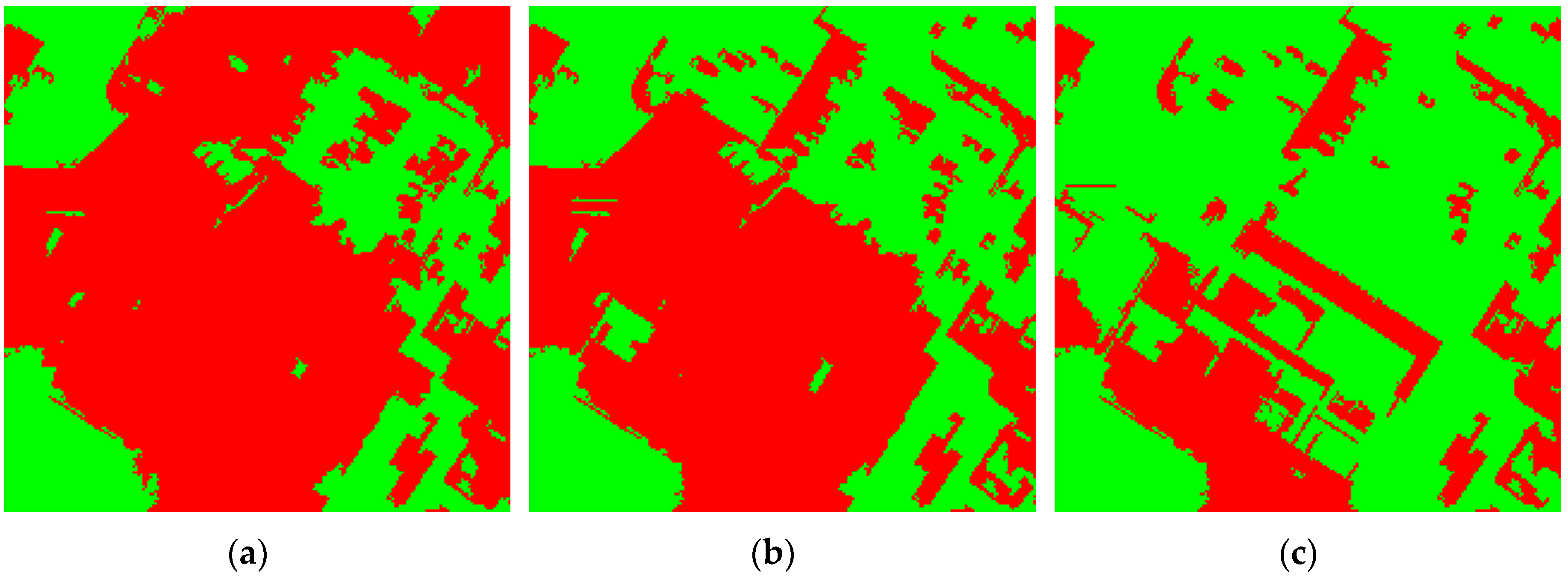Figure 2c shows the obtained changed regions. In Figure 2c, red regions are changed regions and green regions are unchanged regions. Most of buildings are recognized as changed regions. Figure 2d shows the generated mask image, where values of pixels in the changed regions remain unchanged. 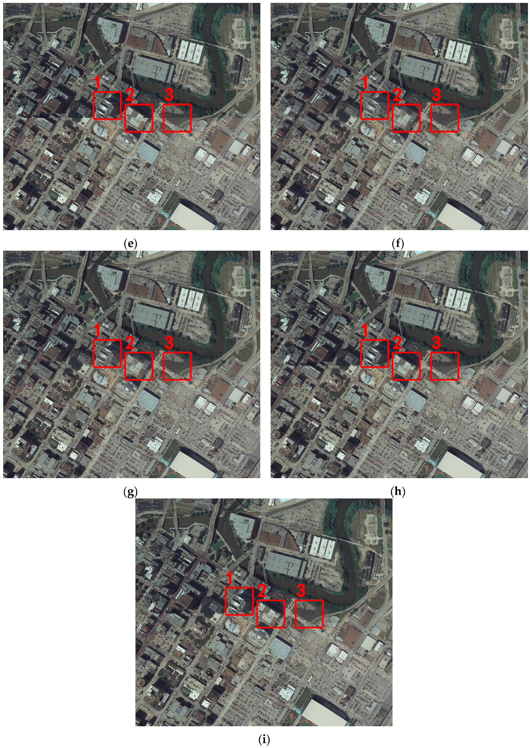Figure 2e–i shows the results of the direct mosaic, the linear ramp weighting method, the cosine distance weighted blending method, the pyramid blending method, and the presented method, respectively.

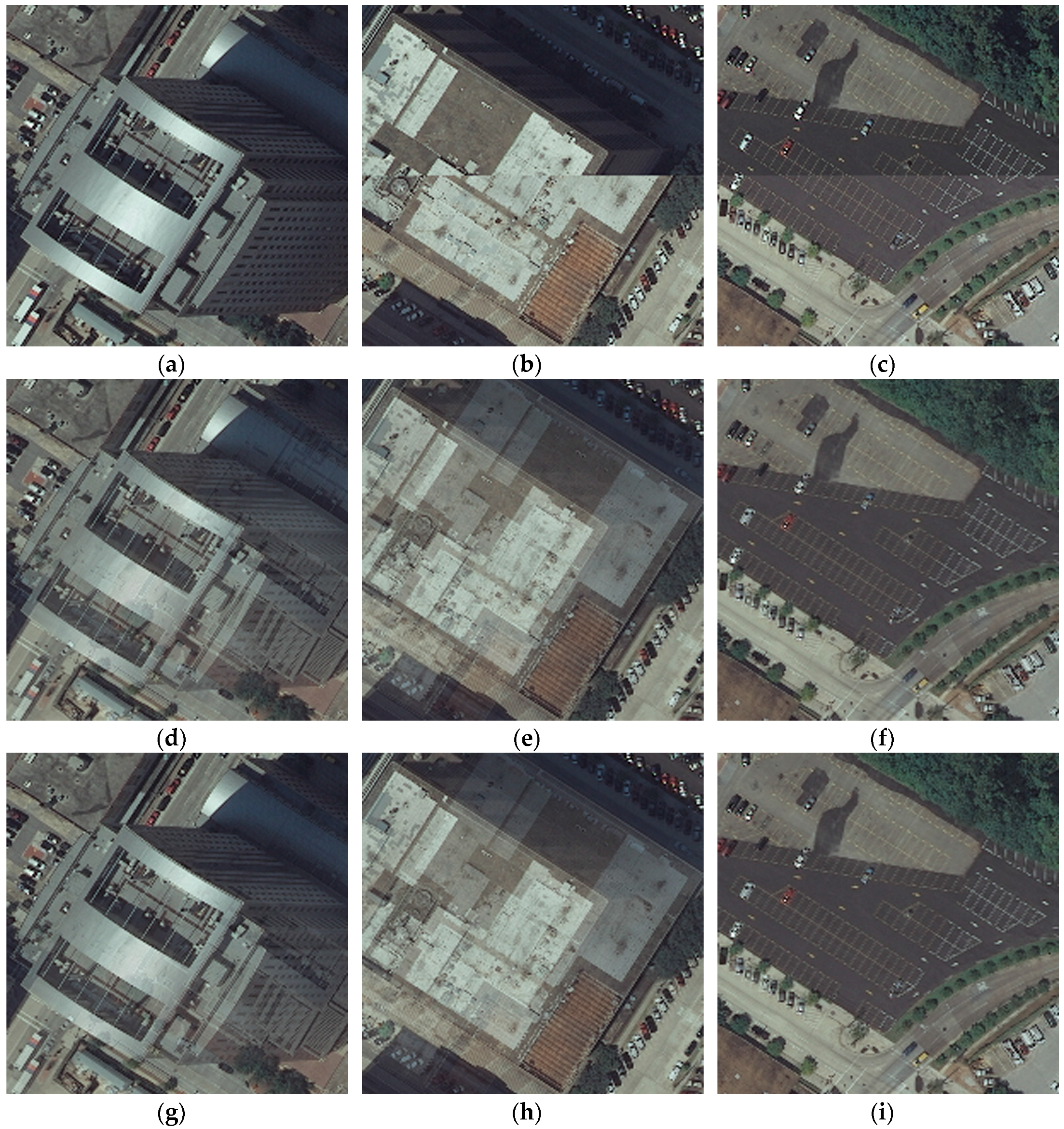
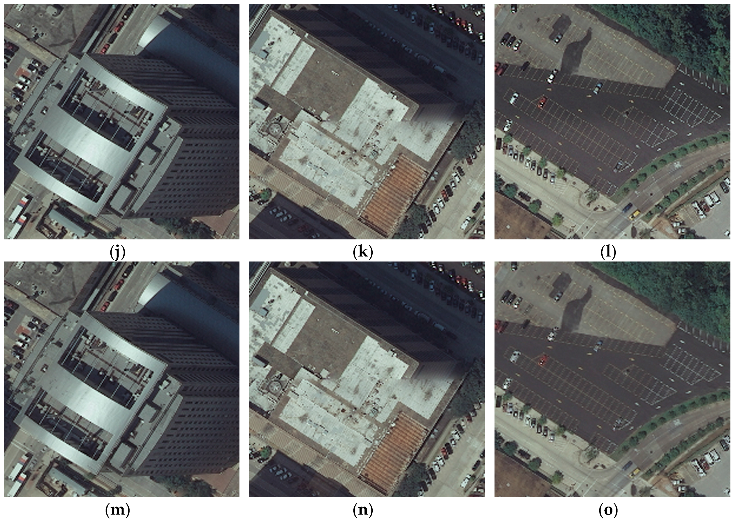
Marked areas 1, 2, and 3 in Figure 2 denote three typical cases of the seamline passing by buildings, the seamline passing through buildings, and the seamline passing through areas with large radiometric differences, respectively. Details of these three cases are shown in Figure 3. In Figure 3, marked areas of the direct mosaic, the linear ramp weighting method, the cosine distance weighted blending method, the pyramid blending method and the presented method are shown from top to bottom. The linear ramp weighting method achieves a smooth transition in the given blending width when the seamline passes through areas with large radiometric differences (Figure 3f). However, ghosting and artifacts also appear when the seamline passes by buildings (Figure 3d) or through buildings (Figure 3e). The cosine distance weighted blending method also obtains a smooth transition when the seamline passes through areas with large radiometric differences (Figure 3i), and ghosting and artifacts are less than the linear ramp weighting method when the seamline passes by buildings (Figure 3g) or through buildings (Figure 3h) due to the improved weight function. The pyramid blending method avoids ghosting and artifacts when the seamline passes by buildings (Figure 3j) or through buildings (Figure 3k), but the transition is not smooth when the seamline passes through areas with large radiometric differences (Figure 3l). The presented method avoids the shortcomings of the linear ramp weighting, the cosine distance weighted blending method and the pyramid blending methods, and performs well in these three cases (Figure 3m–o).

A quantitative comparison was also conducted. The correlation coefficient was utilized to evaluate the ability to preserve detailed information in the image, with the direct mosaic as a reference.

Table 1. Correlation coefficient comparison for data set 1.

Methods	Red	Green	Blue
the linear ramp weighting method	0.969	0.989	0.968
the cosine distance weighted blending method	0.972	0.992	0.971
the pyramid blending method	0.979	0.999	0.978
the presented method	0.977	0.997	0.976

shows comparison of the correlation coefficient between the results of the direct mosaic and the linear ramp weighting, the cosine distance weighted blending method, the pyramid blending, and the presented methods in each channel for data set 1. The linear ramp weighting method had the smallest correlation coefficient value in each channel due to ghosting and artifacts. The cosine distance weighted blending method had larger correlation coefficient value in each channel than the linear ramp weighting method. The pyramid blending method had the largest correlation coefficient value in each channel because of its narrow blending width. The presented method obtained correlation coefficient values close to that of the pyramid blending method. The comparison indicated that the ability to preserve detailed information of the presented method was better than the linear ramp weighting method and the cosine distance weighted blending method, and very close to that of the pyramid blending method. Considering the poor performance of the pyramid blending method when the seamline passes through areas with large radiometric differences, the presented method obtained the best outcome.

This paper also presents another data set, i.e., data set 2, to demonstrate the performance of the presented method. The image size of data set 2 is approximately 2800 by 2300 pixels. Figure 4 and Figure 5 show comparisons of the direct mosaic, the linear ramp weighting method, the cosine distance weighted blending method, the pyramid blending method and the presented method. The parameters of these methods are the same as data set 1. The left and right images overlapping seamlines (dotted line) are shown in Figure 4a,b, respectively. 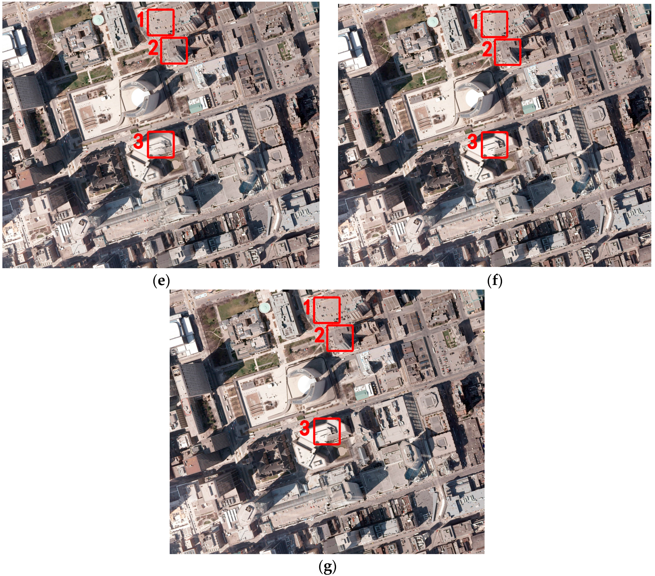Figure 4c–g shows the results of the direct mosaic, the linear ramp weighting method, the cosine distance weighted blending method, the pyramid blending method, and the presented method, respectively.

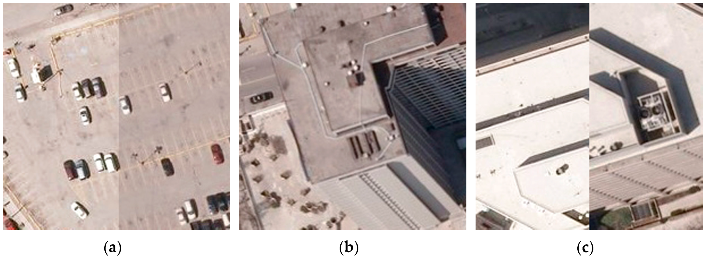
Marked areas 1, 2, and 3 in Figure 4 denote three typical cases of the seamline passing through areas with large radiometric differences, the seamline passing by buildings, and the seamline passing through buildings, respectively. Details of these three cases are shown in Figure 5. In Figure 5, marked areas of the direct mosaic, the linear ramp weighting method, the pyramid blending method and the presented method are shown from top to bottom. The linear ramp weighting method obtains a smooth transition in the given blending width when the seamline passes through areas with large radiometric differences (Figure 5d), but there are still ghosting and artifacts (marked areas in Figure 5d) because there is a moving white car. More obvious ghosting and artifacts appear when the seamline passes by buildings (Figure 5e), and when the seamline passes through buildings (Figure 5f). The cosine distance weighted blending method obtains similar result to the linear ramp weighting method (Figure 5g–i). Of course, ghosting and artifacts created by the cosine distance weighted blending method are less than the linear ramp weighting method when the seamline passes by buildings (Figure 5h) or through buildings (Figure 5i). The pyramid blending method successfully avoids ghosting and artifacts in these three cases (Figure 5j–l), but the transition is not smooth when the seamline passes through areas with large radiometric differences (Figure 5j). 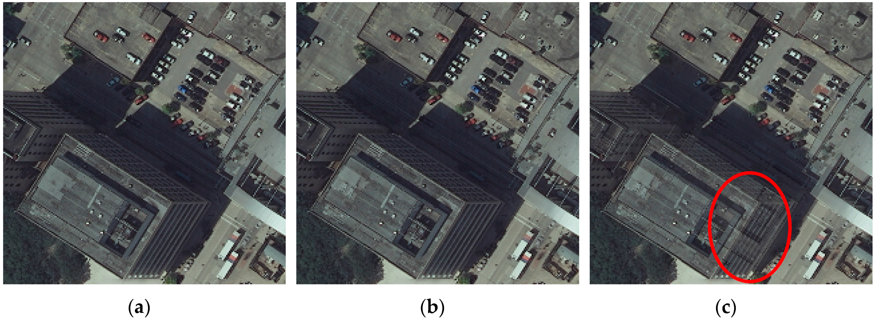The presented method avoids shortcomings of the other three methods and performs well in these three cases (Figure 5m–o). Of course, there are also flaws with the presented method. As shown in Figure 5n, there is still ghosting in the building areas.

Table 2. Correlation coefficient comparison for data set 2.

Methods	Red	Green	Blue
the linear ramp weighting method	0.975	0.995	0.976
the cosine distance weighted blending method	0.977	0.997	0.978
the pyramid blending method	0.980	0.999	0.980
the presented method	0.979	0.999	0.979

shows comparison of correlation coefficient between in each channel for data set 2. The linear ramp weighting method had the smallest correlation coefficient in each channel. The cosine distance weighted blending method had larger correlation coefficient value in each channel than the linear ramp weighting method. The pyramid blending method had the largest correlation coefficient value in each channel. The presented method obtained correlation coefficient values close to that of the pyramid blending method. The comparison also indicated that the ability to preserve detailed information of the presented method was better than the linear ramp weighting method and the cosine distance weighted blending method, and very close to that of the pyramid blending method. Considering the poor performance of the pyramid blending method when the seamline passes through areas with large radiometric differences, the presented method also obtained the best outcome in data set 2.

4. Discussion

This paper provided detailed performance of the presented method in blending processing based on seamlines for orthorimage mosaicking in urban areas. To give an overall assessment of the linear ramp weighting [3], the cosine distance weighted blending method [4], the pyramid blending [5], and the presented method, detailed comparisons between these methods in three typical cases of the seamline passing by buildings, the seamline passing through buildings, and the seamline passing through areas with large radiometric difference were also presented.

The linear ramp weighting method always obtained a smooth transition in the given blending width, but if there were projection differences (e.g., the seamline passing by or passing through buildings) or moving objects (e.g., cars) within the blending width, ghosting and artifacts appeared because the linear ramp weighting method was a blind blending procedure [3]. This had been validated by the presented experimental results of the presented two data sets.

The cosine distance weighted blending method obtained similar results to the linear ramp weighting method. Because it improved the weighting function, the cosine distance weighted blending method obtained smoother transition than the linear ramp weighting method near the borders of the transition zone [4]. Thus, ghosting and artifacts generated by the cosine distance weighted blending method were slighter than the linear ramp weighting method.

The pyramid blending method always avoided ghosting and artifacts, but the transition was not smooth when the seamline passed through areas with large radiometric differences. This was mainly because the blending in this method was carried out in a narrow width in fact [5].

The presented method achieved the best outcome considering both the visual effect and the quantitative statistics. This was due to the selective blending strategy for changed and unchanged regions. It was implemented in the generation of the mask image. For changed regions, if the seamline passed by or through them, blending would be avoided or limited in a narrow width, which is similar to the pyramid blending method. For unchanged regions, if the seamline passed by or through them, blending would be carried out in the set blending width to achieve a smooth transition, which is similar to the linear ramp weighting method.

Of course, the presented method also has its shortcomings. A key step of the presented method is to distinguish changed and unchanged regions. Whether regions of buildings and moving objects can be accurately determined as changed regions has an important impact on the performance of the presented method. As shown in Figure 5n, because the color of the building roof is very similar to that of the road and the boundary of the building roof is unclear, the building roof and the road are segmented into the same region, so there is still ghosting in the building areas. The determination of changed regions is dependent on image segmentation and change detection. However, there is still no automatic solution to selecting proper segmentation and change detection parameters at present. In practice, what we have done was to choose certain typical images and test which parameters would produce suitable results. Then, the selected parameters were applied to other images.

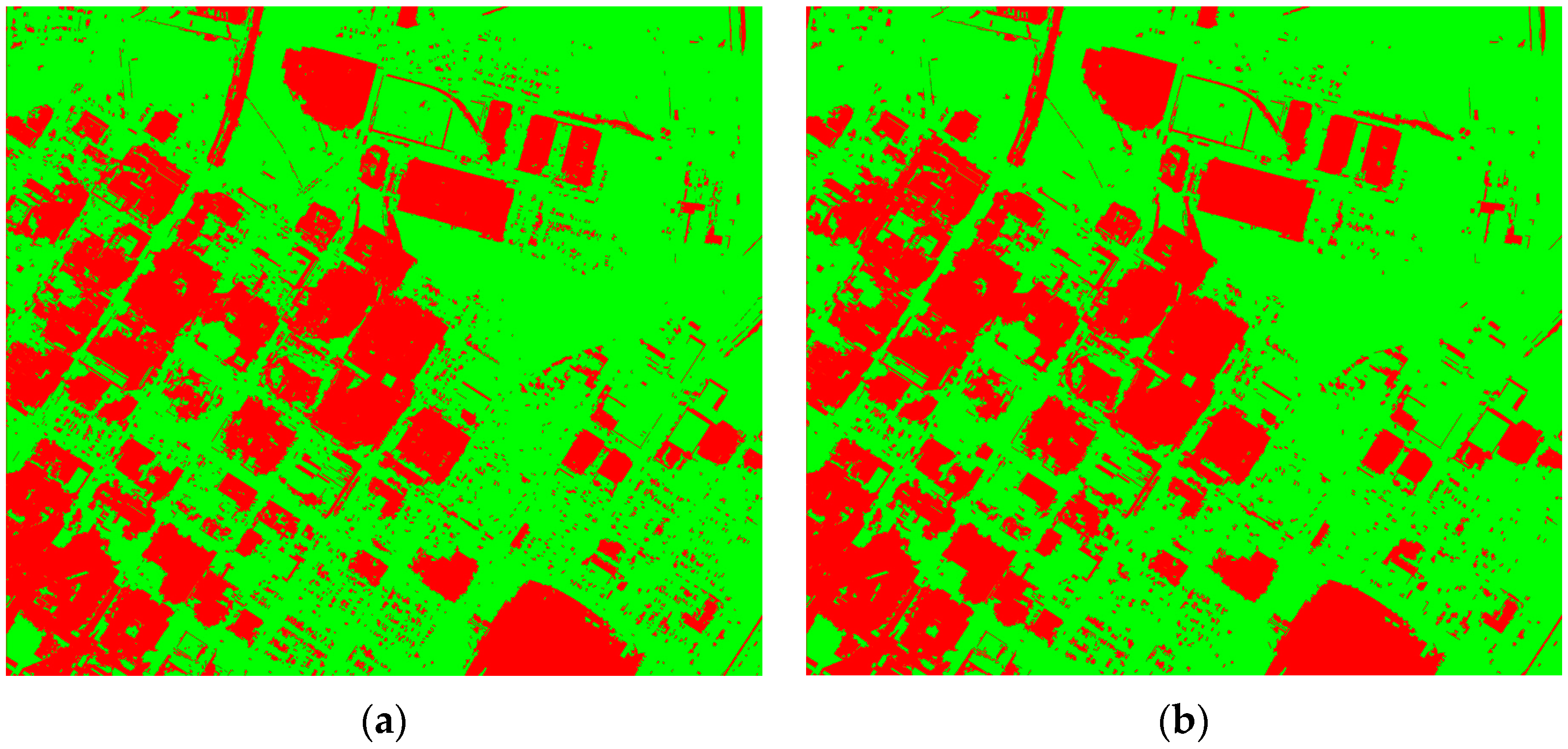
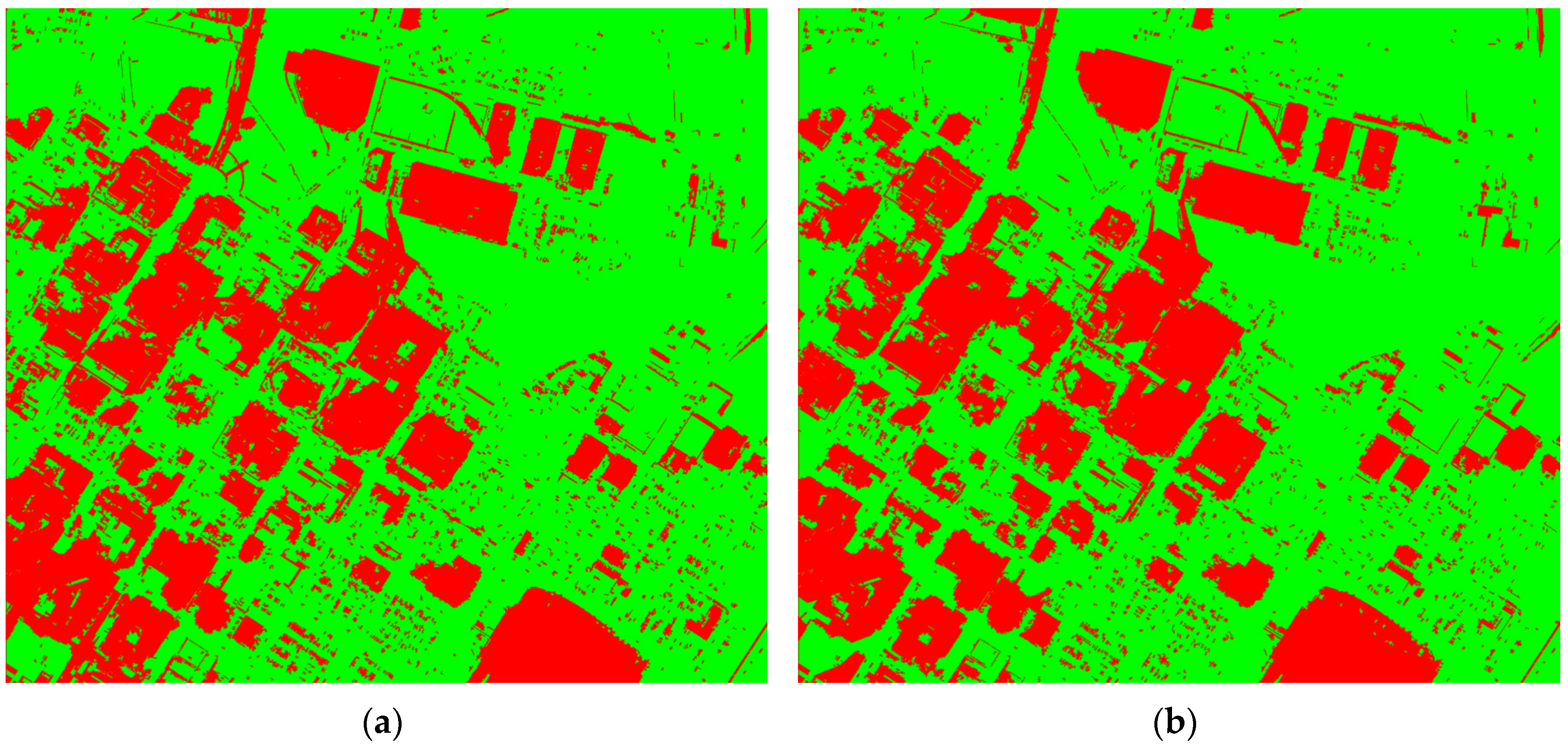
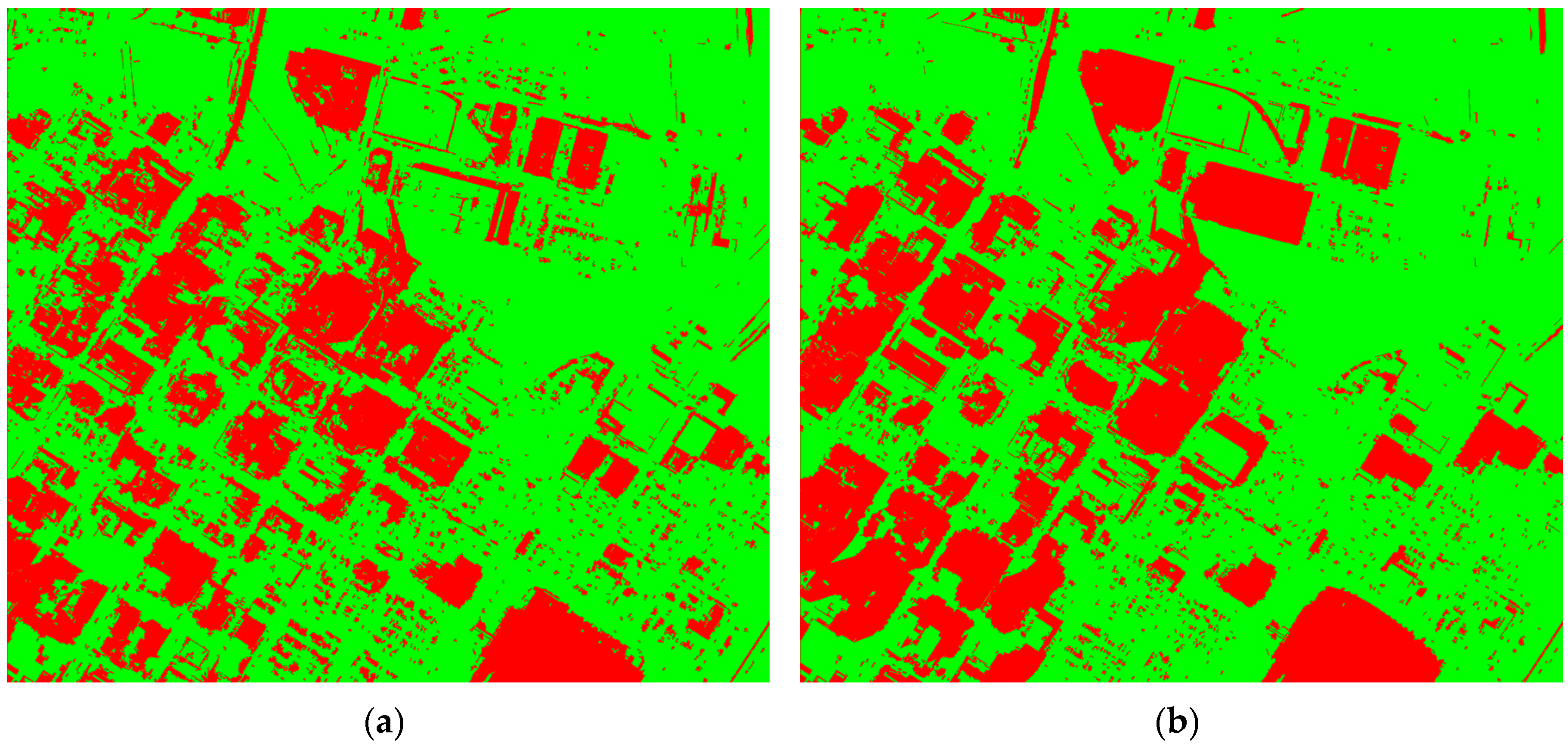
The threshold of RCR, $TRate$, should be moderate. In our experiments, $TRate$ is set to 0.2. From our experience, the presented method is slightly sensitive to the value of $TRate$. Figure 6 shows obtained changed regions with $TRate=0.1$ (Figure 6a) and $TRate=0.3$ (Figure 6b) for data set 1 respectively. Figure 7 shows details of changed regions when $TRate=0.1$, $TRate=0.2$ and $TRate=0.3$ respectively. Figure 8 further shows corresponding detailed results of the presented method when $TRate=0.1$, $TRate=0.2$ and $TRate=0.3$ respectively. Obviously, compared with $TRate=0.2$, more regions are considered as changed regions when $TRate=0.1$ and less regions are considered as changed regions when $TRate=0.3$. When $TRate=0.3$, only parts of buildings are considered as changed regions, so there are still ghosting and artifacts in building areas after blending. As shown in Figure 8c, ghosting and artifacts are very obvious especially in the marked ellipse areas. When $TRate=0.1$ and $TRate=0.2$, blending results (Figure 8a,b) are similar and satisfied. Thus, relative small value of $TRate$ can achieve better result. Of course, too small value of $TRate$ is also not suitable because if $TRate$ is smaller, more regions will be considered as changed regions and the presented method will be more similar to the pyramid blending method [5].

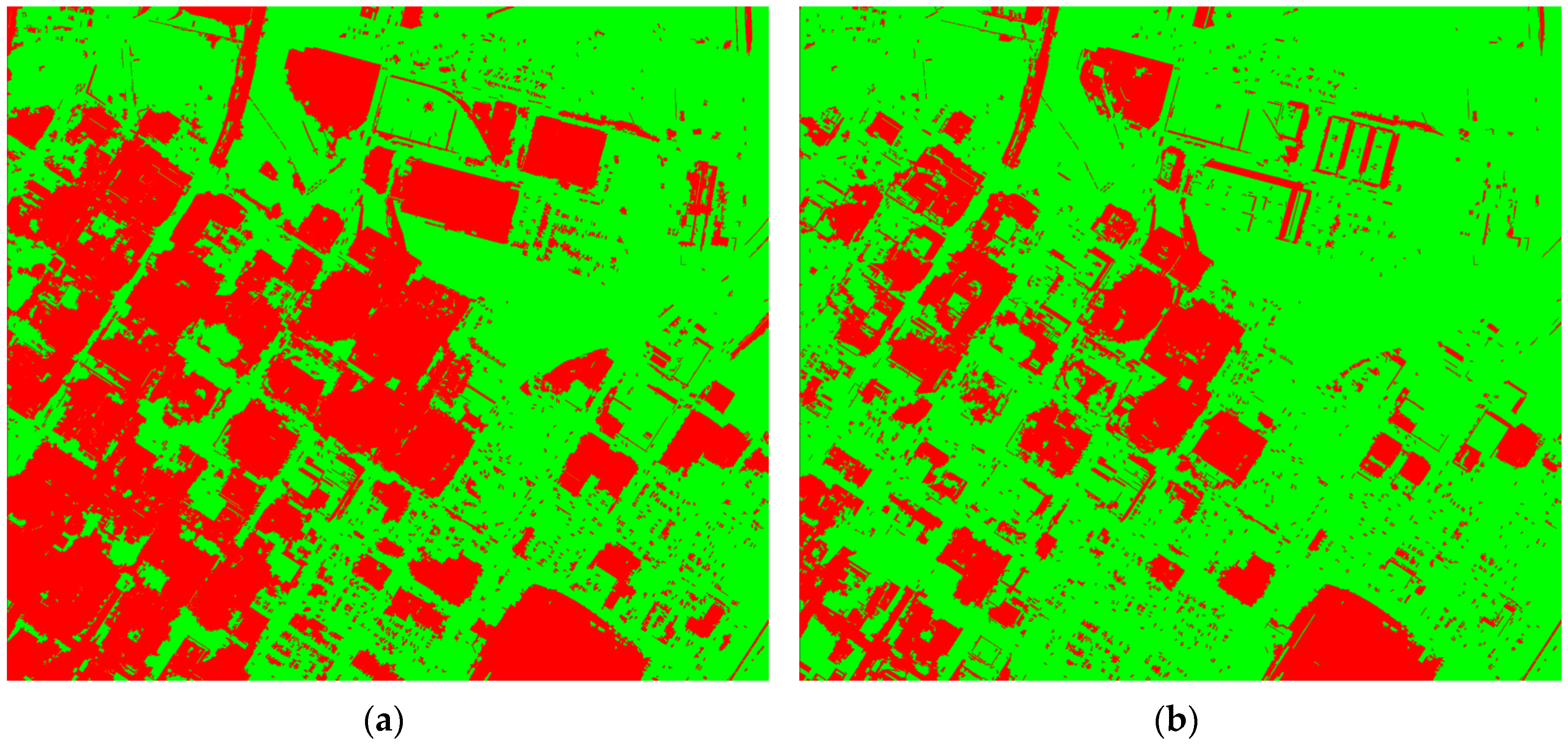
Different parameters of MS algorithm $(h_s,h_r,M)$ are also set to analyze the sensitivity of the presented method. The presented method is not sensitive to the value of $M$ because it yields almost the same changed regions for different values of $M$ (compare Figure 9a,b and Figure 2c) and if changed regions are same, the blending results are also identical. However, the presented method is slightly sensitive to the values of $h_s$ and $h_r$. Where for different values of $h_s$, results yielded by the presented method are slightly different. Though obtained regions are similar with different values of $h_s$ (compare Figure 10a,b and Figure 2c), details of blending results are still slightly different. 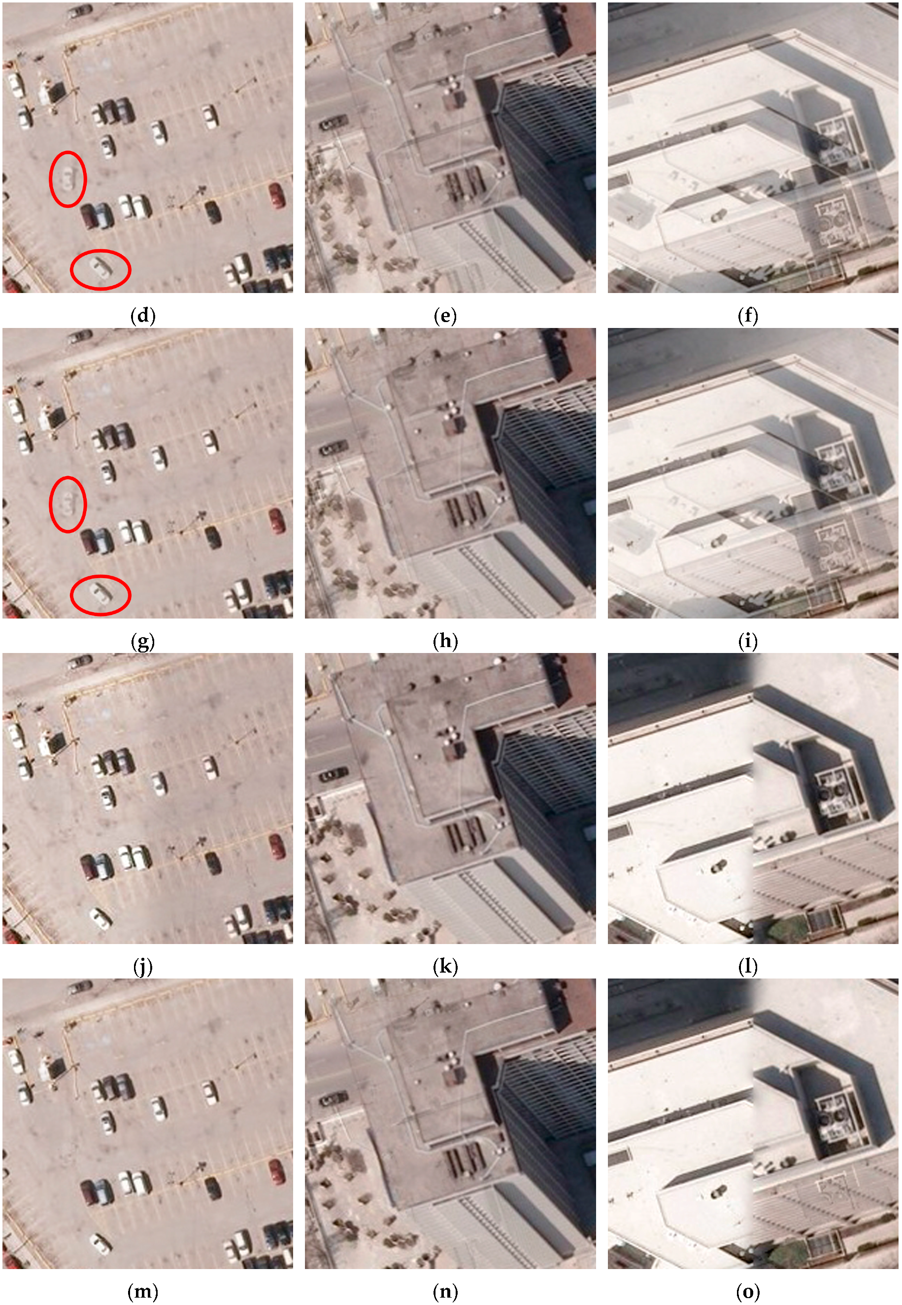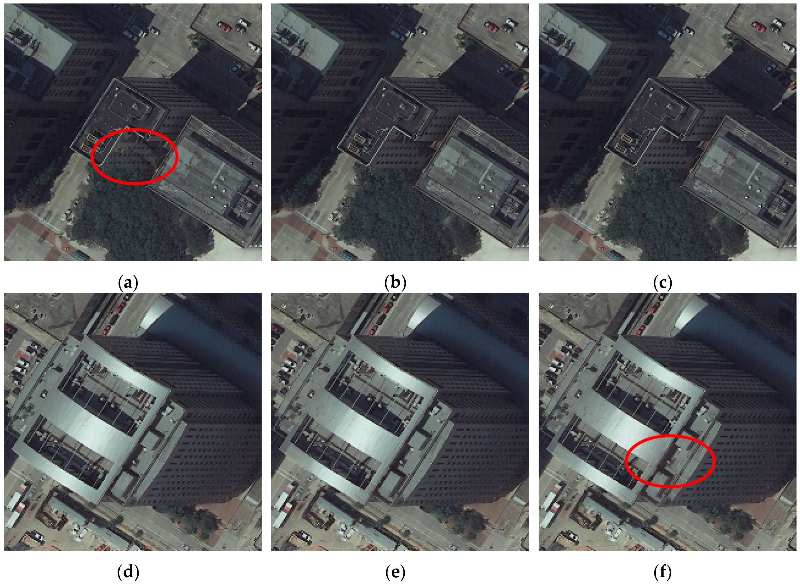Figure 11a–c shows one selected region of blending results when $(h_s,h_r,M)$ = (3, 5, 20), $(h_s,h_r,M)$ = (6, 5, 20), and $(h_s,h_r,M)$ = (9, 5, 20) respectively. Obviously, there are still some ghosting and artifacts when $(h_s,h_r,M)$ = (3, 5, 20) (marked ellipse areas in Figure 11a). Figure 11d–f shows another selected region of blending results when $(h_s,h_r,M)$ = (3, 5, 20), $(h_s,h_r,M)$ = (6, 5, 20), and $(h_s,h_r,M)$ = (9, 5, 20) respectively. Obviously, there are also some ghosting and artifacts when $(h_s,h_r,M)$ = (9, 5, 20) (marked ellipse areas in Figure 11f). As far as $h_r$ is concerned, results are also slightly different for different values. As show in Figure 12, obtained regions are slightly different with different values of $h_r$. When $(h_s,h_r,M)$ = (6, 2.5, 20), changed regions are more dispersed, and when $(h_s,h_r,M)$ = (6, 7.5, 20), changed regions are more concentrated. Figure 13 further shows selected regions of blending results with $(h_s,h_r,M)$ = (6, 2.5, 20), $(h_s,h_r,M)$ = (6, 5, 20), and $(h_s,h_r,M)$ = (6, 7.5, 20) respectively. Obviously, there are still some ghosting and artifacts when $(h_s,h_r,M)$ = (6, 2.5, 20) and $(h_s,h_r,M)$ = (6, 7.5, 20) (marked ellipse areas in Figure 13a,c).

5. Conclusions

Blending processing based on seamlines is an important step for orthoimage mosaicking. This paper presents a novel method of multi-resolution blending considering changed regions to improve mosaic image quality. The presented method is an improved pyramid blending method and the improvement lies mainly in the mask image generation. Unlike the pyramid blending method in [5], the presented method enlarges the transition zone width by adding a smooth filter to the mask image. When generating the mask image, changed pixels and unchanged pixels are first distinguished according to texture similarity, and the overlaps in the left and right images are segmented separately by MS. Then, the RCR of each segmented region in the overlap can be computed based on the percentage of changed pixels in the segmented region. After calculating the RCR for each segmented region, a threshold of the RCR is set to determine if a region belongs to a changed region. Regions with obvious projection differences or moving objects are considered as changed regions. When adding a smooth filter on the mask image, values of pixels in changed regions remain unchanged. Thus, in the blending procedure, if the seamline passes through changed regions, blending will be limited in a narrow width; if the seamline passes by changed regions, blending will be avoided; and, if the seamline passes through or by unchanged regions, blending will be carried out in the set blending width to achieve a smooth transition. By doing so, the mosaic of orthoimages not only is a true reflection of earth’s surface but also has a good visual effect. Experimental results and comparison with other methods indicate the potential of the presented method. Different parameters of MS algorithm and the threshold of RCR are also set to analyze the sensitivity of the presented method. The presented method only deals with the case of two images with overlaps. If there are more than two images with overlaps, it is also easy to use the presented method to do the blending processing. The simplest way is to do the blending processing sequentially, i.e., only two images are blended each time. Brown and Lowe (2007) gave a more complex way [7]. Of course, other available image segmentation methods may achieve better efficiency and have easier parameter selection. Other advanced change detection methods may distinguish changed and unchanged pixels more effectively. Additionally, the selection of parameters for image segmentation and change detection automatically and effectively to achieve accurate changed regions also may improve the blending effect. These issues will also be studied in the future work.