Article

Urban Land Cover Change Modelling Using Time-Series Satellite Images: A Case Study of Urban Growth in Five Cities of Saudi Arabia

by
Abdullah F. Alqurashi
1,2,*,
Lalit Kumar
1 and
Priyakant Sinha
1
1
School of Environmental and Rural Science, University of New England, Armidale NSW 2351, Australia
2
Department of Geography, Umm Al-Qura University, Makkah 21955, Saudi Arabia
*
Author to whom correspondence should be addressed.
Remote Sens. 2016, 8(10), 838; https://doi.org/10.3390/rs8100838
Submission received: 22 August 2016 / Revised: 19 September 2016 / Accepted: 4 October 2016 / Published: 13 October 2016

Abstract

:
This study analyses the expansion of urban growth and land cover changes in five Saudi Arabian cities (Riyadh, Jeddah, Makkah, Al-Taif and the Eastern Area) using Landsat images for the 1985, 1990, 2000, 2007 and 2014 time periods. The classification was carried out using object-based image analysis (OBIA) to create land cover maps. The classified images were used to predict the land cover changes and urban growth for 2024 and 2034. The simulation model integrated the Markov chain (MC) and Cellular Automata (CA) modelling methods and the simulated maps were compared and validated to the reference maps. The simulation results indicated high accuracy of the MC–CA integrated models. The total agreement between the simulated and the reference maps was >92% for all the simulation years. The results indicated that all five cities showed a massive urban growth between 1985 and 2014 and the predicted results showed that urban expansion is likely to continue going for 2024 and 2034 periods. The transition probabilities of land cover, such as vegetation and water, are most likely to be urban areas, first through conversion to bare soil and then to urban land use. Integrating of time-series satellite images and the MC–CA models provides a better understanding of the past, current and future patterns of land cover changes and urban growth in this region. Simulation of urban growth will help planners to develop sustainable expansion policies that may reduce the future environmental impacts.

Graphical Abstract

1. Introduction

Urbanization has a significant effect on the ecosystem components and is a key factor in global environmental change [1]. The expansion of urbanization is a response to world population growth and its consequences involve the transformation of natural forms of land cover into urban areas [2]. The world population has rapidly increased from 244 million in 1900 to 7 billion in 2011 and is expected to exceed 9.3 billion by 2050 [3]. Most of the population growth will occur in the urban areas [4] and most of the net increase will be in the cities of developing countries [4]. Human developments in urban areas have resulted in a serious modification of and threat to the landscape’s ecosystem and natural diversity [5,6], and cause changes in the ecological and environmental components [7]. Measuring past spatiotemporal dynamics of urban cover and predicting patterns of future change can provide much needed information for planners and resource managers to enable sustainable development that takes into account the management of natural resources and environmental conservation.
Remote sensing data and methods provide the essential information regarding identifying, mapping, assessing, monitoring and modelling the spatial, temporal and thematic scales of various land cover features [8,9], including urban growth [10,11]. The spatial time-series data provided by Remote Sensing (RS) systems serve as an excellent source to analyse and quantify the changes over time in different urban cover and other land cover types. The repetitive coverage, cost effectiveness and accessibility of RS data offer great potential in terms of identifying and modelling long-term urban changes [12,13,14]. A number of studies have utilized bi-temporal RS data to detect the spatial patterns and overall rate of urban cover change for selected periods of time. For instance, Rahman [15] detected urban land use in eastern coastal city of Al-Khobar, Saudi Arabia between 1990 and 2013 using maximum likelihood classification (MLC) and ISODATA methods to classify Landsat TM, ETM+ and OLI data. Similarly, Pellikka and Alshaikh [16] utilized Landsat TM and ETM+ to map LULC changes and built-up area in Al-Baha southwestern Saudi Arabia between 1984 and 2014 using MLC method. While considerable efforts were made to provide accurate information related to the rate and patterns of urban growth, understanding and quantifying the transition patterns are essential in order to determine the direction and magnitude of urban growth predicted to occur in the future. Given the availability of RS data and the capabilities of different land cover modelling techniques, accurate extraction of past urban cover information allows us to model the change trajectories of urban cover and other land cover types.
Modelling land cover changes requires accurate extraction of both historical and current land-use and land-cover (LULC) information [17], which allow models to evaluate past scenarios and predict future changes. A wide variety of remote sensing methods have been developed and used to extract LULC change information from satellite data. Pixel-based image analysis methods are the most widely used to derive LULC maps [18,19,20]. Recently, object-based image analysis (OBIA) has gained an acceptance among different RS applications and has received a great attention in image classification [21,22,23]. The OBIA method has advantages of including contextual information into the classification process, which can effectively reduce the “salt and pepper” effect and improve the classification accuracy compared to pixel-based classification methods [21,23,24,25].
OBIA technique has been successfully implemented on Landsat images and provided accurate classification for LULC changes in the previous studies. For example, Taubenböck, et al. [26] utilized OBIA technique to monitor urban expansion in 28 mega cities throughout the world using Landsat images. Yu, et al. [23] used OBIA technique and Landsat TM data to classify LULC changes in Beijing, China. Platt, et al. [27] concluded that OBIA classification yielded high average class accuracies compared to traditional pixel-based approaches. For this propose, OBIA and updated classification approaches are utilized to accurately classify LULC changes which are then used as input for the simulation model.
Urban expansion is a dynamic and complex process that involves a number of social, environmental, institutional and economic processes [28] and, therefore, modelling urban dynamics with these driving factors is a challenging task [29]. The role of these factors is defined and then included in the transition rules for the modelling of urban development [30]. In the past, a wide variety of approaches and methods have been applied to model the dynamics of urban cover change and its driving factors [31,32,33,34,35,36,37,38]. Integrating the Markov chain (MC) and cellular automata (CA) techniques has been found to be a suitable approach through which to simulate the spatiotemporal changes in urban cover [2,39,40,41].
The basic assumption of MC model is that the LULC changes are stochastic processes in which different categories of LULC are states of a chain [42,43]. The definition of chain is as a stochastic process, where the value of the process at time t, Xt, only depends on its value at time t − 1, Xt−1 and is not dependent on the sequence of values Xt−2, Xt−3,…X0, which the process passed through before arriving at Xt−1. The expression of chain can be as:
P { X t = A j | X 0 = A 0 , X 1 = A 1 , , X t - 1 = A i } = P { X t = A j | X t - 1 = A i }
The P { X t = A j | X t 1 = A j } is known as the one-step transitional probability, which gives the probability the process that makes the transition from state Ai to Aj in one time period. The P { X t = A j | X t 1 = A j } is called the m-steps transition probability, P i j m when m-steps are required to implement this transition [42]. The MC is said to be homogeneous if the P i j m is independent of time and dependent only upon states Ai, Aj and m. The use of MC treatment in this study will be limited to the first order homogenous and in this case:
P { X t = A j | X t 1 = A i } = P i j
where Pij can be estimated from observed data by tabulating the number of times the observed data went from state i to j and summing the number of times that state Ai occurred.
There are three issues arising where the observed changes violate the assumption of a first order Markov model. Non-stationarity, spatial dependencies and historical matters limit the success of the first order MC due to dynamics of LULC change (more information can be found in [43]). The non-stationarity can be solved by limiting the time span of the historical LULC changes to be short between t − 1 and t − 2 [42]. The use of MC model and CA can resolve the spatial dependencies by combining the concept of MC, CA, Multi-Criteria Evaluation (MCE) and Multi-Objective Land Allocation (MOLA) [35,43,44]. The CA model, hence, controls the spatial patterns of LULC classes through the local rules that are determined by either the neighbourhood configuration or by the transition potential maps [2,45,46]. Thus, integration of MC–CA models gives the opportunity to use the power of both methods to model the dynamics of urban growth. Although the simulation of urban cover using the MC–CA integrated model has been improved in previous research [2,39,41], only a few studies have conducted a comparative study of the urban expansion patterns for different landscapes.
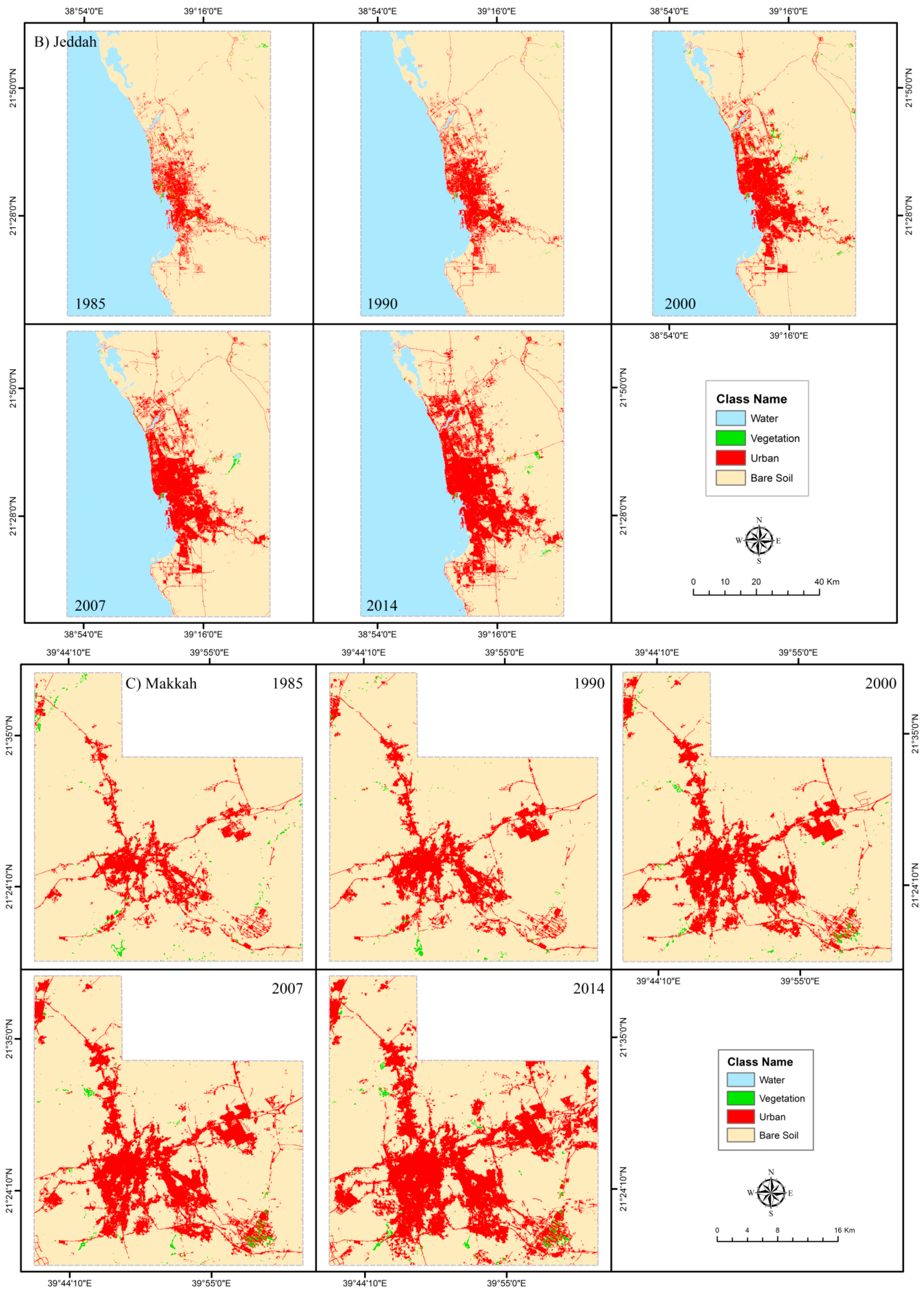
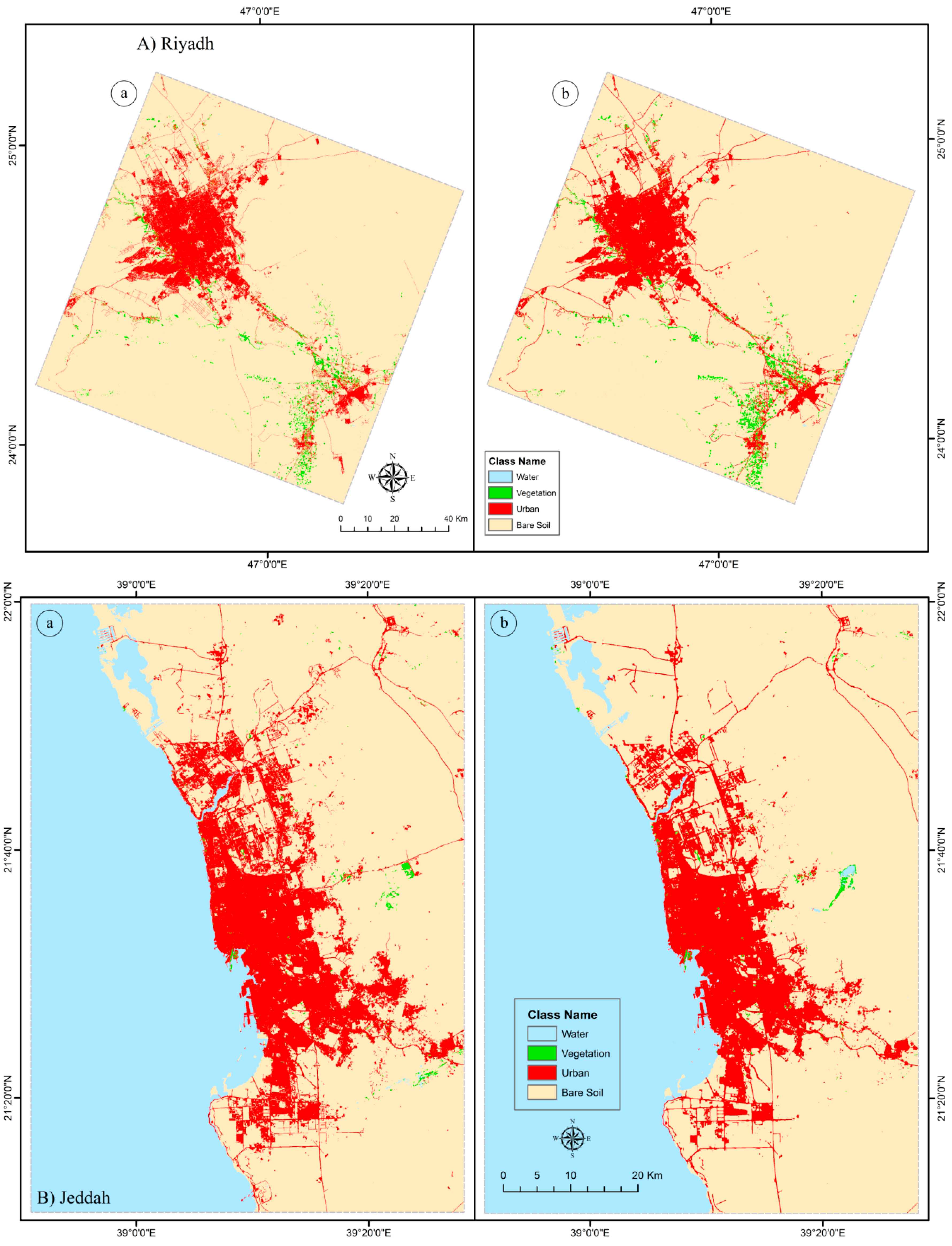
In this research, an integration of time-series satellite images and MC–CA models has been conducted to identify and analyse the patterns of urban expansion in the fast-growing cities of Saudi Arabia. The main aim of this study is to assess the amount and pattern of urban growth in the present and in the past, using RS data between 1985 and 2014 in five Saudi Arabian cities (Riyadh, Jeddah, Makkah, Al-Taif and the Eastern Area). The pattern of LULC in time-series is then used to predict urban growth change scenarios. The objectives of this research are: (1) Urban LULC classification of different change years (1985, 1990, 2000, 2007 and 2014) using OBIA technique for the selected cities; (2) analysis and comparison of the spatiotemporal patterns of LULC changes in relation to urban expansion; (3) determination of transition probabilities of other LULC classes changing to urban area and simulating of changes using MC-CA integrated modelling approach; and (4) based on time-series simulation accuracy, determining future urban expansions for two simulated years 2024 and 2034. The results from this study will provide an overview of past and present urban pattern trends that will help planners and decision makers assess the change pattern in the past and will allow them to prepare and manage the expected future expansion of urbanization to attain sustainability in these cities.

2. Study Areas

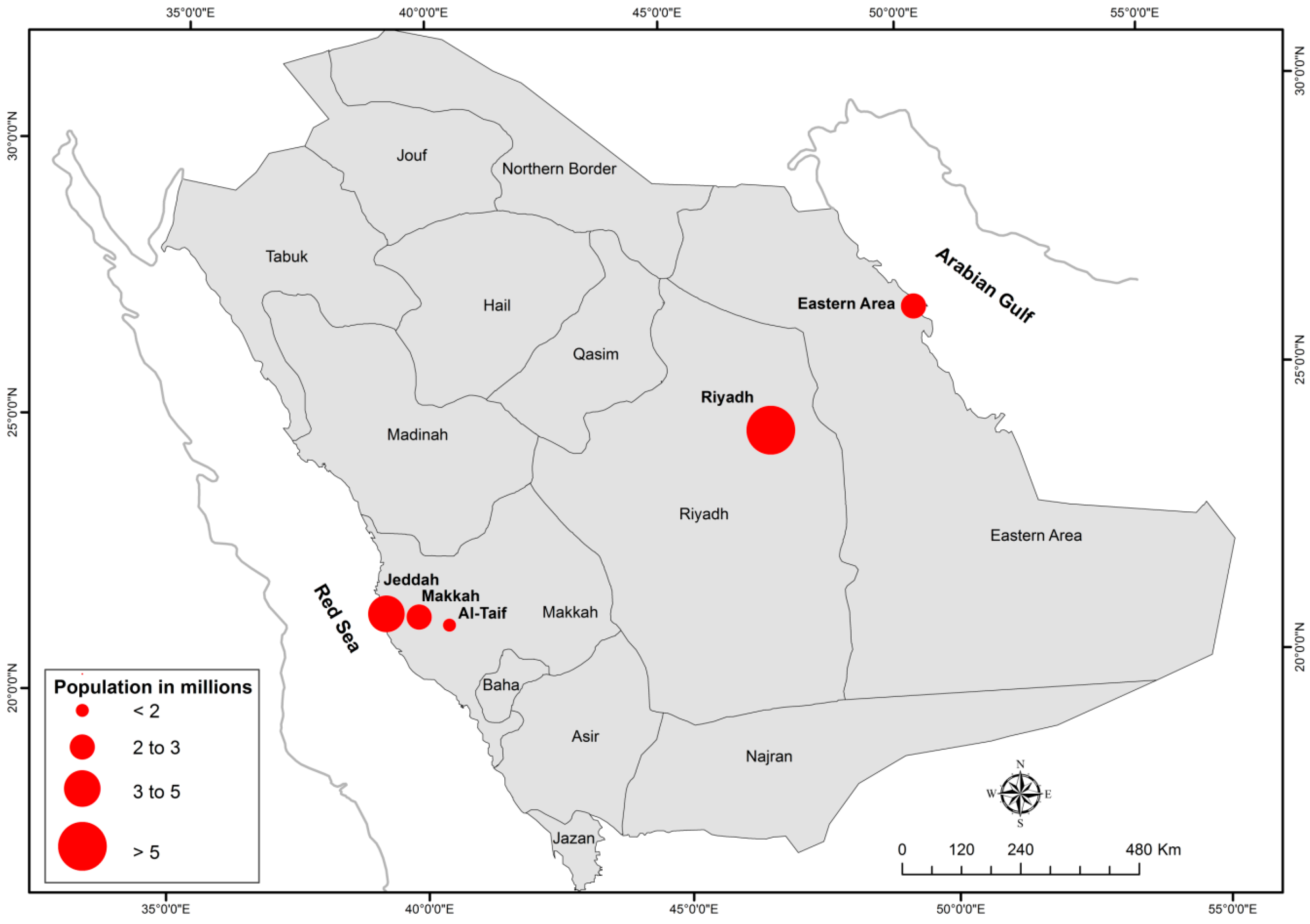
The study areas include five cities of Saudi Arabia: Riyadh, Jeddah, Makkah, Al-Taif and Eastern Area (Figure 1). These cities are considered to be the most urbanized and populated in the country [38]. Riyadh is the capital and largest city, situated in the central part of Saudi Arabia on the large Najd plateau. Al-Kharj city, which is 77 km south-east of Riyadh, is included in the study area. Jeddah is the largest sea port on the Red Sea coast, a major urban centre of western Saudi Arabia and an important commercial hub nationally. It is also the largest city in the western part and the second largest in the country. Makkah is the holy place of the Muslim community and is located in the central part of the region, approximately 70 km inland from Jeddah. Al-Taif, considered to be the most important tourist city of Saudi Arabia [47], is the fourth study area in our analysis and is located in the south-east of Makkah. Eastern Area is located in eastern Saudi Arabia on the Arabian Gulf and is home to most of Saudi Arabia’s oil production. Eastern Area includes 11 towns spread across the region. Only the most populated six towns, which are Dammam, Dhahran, Al-Khobar, Al-Qatif, RasTanura and Al-Jubail, are considered for Eastern Area. Dammam city is in the central part and is the administrative city of the Eastern Area. Table 1 lists the population of 2015 (Central Department Statistics & Information) and the importance of each city.
Most Saudi Arabian cities have faced massive urban growth recently due to an increase in national economics [47,48], which have been used to support the public and private sectors to increase development across the country. The government policy with the natural demographic growth has led to massive changes and increased complexity in the structure of the cities as well as unsystematic development in the last three decades. Migration from the rural to urban centres, for job opportunities, has led to a significant increase in population in these cities. For example, the populations in large cities, such as Riyadh and Jeddah, have increased by 4.6 and 3.0 million respectively between 1985 and 2014 (Central Department Statistics & Information 2015). With such rapid population growth, local authorities and planners face a significant challenge to meet the infrastructure demand and to understand the urban growth process and associated consequences [49]. Therefore, it is important to understand the past and present spatial dimensions for management and for preparing for the future expansion in these cities. Understanding the urban growth process and its patterns is essential to secure sustainable development for future urban growth and to avoid unwanted and negative environmental and ecological consequences.

3. Data and Methods

3.1. Data and Pre-Processing

A total of 30 Landsat thematic mapper (TM), enhanced thematic mapper plus (ETM+) and operational land imager (OLI) images were collected from the United States Geological Survey (USGS) Global Visualization (GloVis) site for the five cities. The acquisition data ranged between spring and summer from March to November, except for the 1985 images for Riyadh, (path 165 and 166 and row 43), which were collected during winter (January) (Table 2). All of the images were georeferenced as level 1 products; however, the TM images (path 164 and row 42 and path 165 and row 43) of the Eastern Area and Riyadh, respectively, were not correctly georeferenced. An automatic image-to-image registration was applied using Landsat OLI images of a similar path and row as base images and Landsat TM images were employed as wrap images. Mosaic processing was applied to merge two path and row images for Riyadh and the Eastern Area. Finally, image subsets were extracted for the five cities, including all of the urban boundaries across the five cities. The entire image processing tasks were carried out using ENVI 5.1 software.

3.2. Image Segmentation and Classification

OBIA was used to create LULC classifications for years 1985, 1990, 2000, 2007 and 2014. The OBIA process consisted of image segmentation and classification, which was carried out using eCognition Developer 8.9 software [50]. The segmentation and classification procedures were applied first on the 1985 Landsat image which was then used as a reference image to classify the next period (1990). The multi-resolution segmentation algorithm was applied to create objects that delineated LULC classes. Two levels for the segmentation and classification processes were created based on land cover patches. The level-1 was created for relatively small land cover patches, such as vegetation cover for all five cities and also for water in Riyadh, Makkah and Al-Taif. The scale parameter setting was 5 for this level. The level-2 was created for the large land cover patches, such as urban area and bare soil in all five cities and also water for coastal cities (Jeddah and Eastern Area). The scale parameter was set at 10 for this level. The other two parameters, colour and shape, were adjusted to 0.9 and 0.1 respectively, as suggested by previous studies for better segmentation results [23,51,52].
The classification of segmentation objects was started with the 1985 image based on the defined rules and threshold values. The classification was divided into four land cover categories, water (W), vegetation cover (VC), bare soil (BS) and urban area (UA), in the class hierarchy (Table 3). The feature sets used to create land cover classes were based on the spectral patterns of Landsat TM bands, Normalized Difference Vegetation Index (NDVI), Normalized Difference Water Index (NDWI) and brightness (the mean of 6 TM bands). Following the previous studies [23,26,53,54], the threshold values of the feature sets were defined. The classification map of 1985 was then used as a thematic layer (reference) for the classification of 1990 image. For each land cover class, the objects with no changes (NC) from 1985 to 1990 were classified as “NC” followed by the class name (e.g., NC–W, NC–VC, etc.). Objects with changes were classified according to the new state of 1990. For example, objects classified as W in 1985 and changed to BS, were then assigned as W–to–BS. At the end of these processes, 13 subclasses were created. Three subclasses were assigned to each class of W, VC and BS and four subclasses were assigned to UA class. Finally, the subclasses were merged and classified into the assigned class, which produced the final 1990 classification. Following similar processes of the 1990 classification analysis, the 2000, 2007 and 2014 images were classified and produced for all five cities.

3.3. Accuracy Assessment

To attain the desired classification accuracy, first a 2016 SPOT 7 image of 1.5 m spatial resolution was used to generate stratified random sampling for each LULC class. The samples were then used for the 2014 image classification and accuracy evaluation, assuming that not much change occurred in the two years’ time. Care was taken to take a large number of samples and also note possible dynamic land cover types, such as vegetation cover, that could have changed between images of 2016 and 2014 and only unchanged samples were used. At the end, 822 samples for Riyadh and other large cities (Jeddah and Eastern Area) and 531 samples for the other two cities were finalized for accuracy evaluation for the year 2014. However, in the absence of reference data of past years, these samples could not be used directly for other change years (2007, 2000, 1990, and 1985) accuracy evaluation because of larger year gaps between the change years. To use these samples as dependent samples, Foody [55,56] suggested a process called signature extension, which allows to use samples for unchanged areas for such purposes. The method was found effective and has been used in several studies (e.g., [57,58]).
For this study, additional processing was undertaken to include sample sites that had not changed during these periods. The NDVI of each year was computed and a difference image was generated by subtracting each year NDVI from 2014 NDVI (e.g., NDVI 2014–NDVI 2007 and so on). The NDVI image was used for this purpose as it reflects both vegetation and non-vegetation areas. On the change image, a threshold of ±1 standard deviation was used to separate change/no-change areas as unchanged pixels were usually clustered about the mean of the difference histogram distribution, while changed pixels were found within the tails. The 2014 samples were overlaid on this change/no-change image, and only samples falling in unchanged area were used for accuracy evaluation. The process was repeated for other change images and signature refinement was done accordingly. The process allowed us to evaluate time-series classification results in the absence of historical reference data. Thus, the sample points for other periods were adjusted to 782, 751, 702 and 679 for large cities and 498, 443, 414 and 382 for the other two cities (Makkah and Al-Taif) for the 2007, 2000, 1990 and 1985 images, respectively. The classifications were compared with respect to the reference points and the error matrix was computed to calculate the overall accuracies and the Kappa statistics for time change periods.

3.4. LULC Change Modelling

3.4.1. MC Model

The classified images of 1985, 1990, 2000, 2007 and 2014 were used to model the LULC changes using the MC method (Figure 2). The MC technique computes the transition matrix for each land cover feature between two time periods. The MC method is a stochastic process [42,43,59] that identifies the probability of the transition of a LULC class from one state to another (e.g., the transition probability of the conversion from bare soil to urban area and so on) within a given time [40]. The outputs of the MC model contain two transition matrices and a set of conditional probability images [60]. The two types of transition matrices are the transition probability matrix and transition area matrix. The transition probability matrix represents the probability of a LULC class changing to another class. The transition area matrix represents the number of pixels that are likely to change from one class to another class over the selected time period [60]. In this study, the transition probabilities were calculated for four change periods (Figure 2). To avoid non-stationarity in the land-cover data, the time span between observation dates is reasonably short [42]. The time intervals used for calibration were 5, 10, 7 and 7 years for the 1985 to 1990, 1990 to 2000, 2000 to 2007 and 2007 to 2014 spans, respectively.

3.4.2. Integrating MC and CA Models

The MC model is not able to provide spatial characteristics to change probabilities [28,43]. Thus, the CA and the MC models were integrated to control the spatial dynamics of LULC changes. The CA model mainly depends on the current state of a cell, its neighbourhood cells and the transition rules that are applied through time and space to predict the state of that cell and its neighbourhood cells in the future. In this study, the transition area matrices and LULC base maps along with the transition suitability maps of each land cover class were used to model the LULC changes using the MC–CA integrated model. The transition area matrix for the period 1985–1990 with 1990 as the base land cover map and the 1990 transition suitability maps were used to predict LULC changes for the year 2000 (Figure 2). Similarly, for the 2007 prediction, the transition area matrix for the period of 1990–2000 and 2000 LULC map as the base along with the transition suitability maps of the 2000 LULC maps were used. The process was repeated for other change years 2014, 2024 and 2034 predictions for each city. The number of iterations selected was based on the number of time steps (years gap) that were used to predict the LULC changes. By using the MOLA procedure, the transition areas were divided by the number of iterations. The results of each MOLA operation were overlaid to produce the prediction for the new LULC maps at the end of each iteration [60]. The CA filter for the suitability of each pixel for the LULC classes was weighted using a contiguity filter type. The standard filter of 5 × 5 pixels was used to define the neighbourhood rules.

3.4.3. Transition Suitability Maps

The transition suitability maps of each LULC class were generated using five variables or factors. These factors were elevation, slope, distance from drainage, distance from roads and distance from urban cover. The elevation, slope and drainage were calculated using a 30 m digital elevation model (DEM) for each city [61], with an accuracy of ±20 m [62]. The distances from roads and from drainage were calculated using the Euclidean distance algorithm. Road layers were delineated using heads-up digitizing from the time-series Landsat images for each year from 1985 to 2014. The distance to urban cover was generated by extracting the urban class from the LULC images and running the Euclidean distance algorithm on the output. Figure 3 shows an example of factors that were used to create the suitability maps in Jeddah.
A fuzzy set function was used to evaluate the possibility of the suitable locations (pixels) of the five factors having an effect on the LULC classes. For each factor, visual analysis was carried out to examine its effect by overlaying the urban cover and each factor individually and when satisfied, the values of each factor were adjusted based on the current state of urban growth. For example, the effect of elevation was evaluated by overlaying the urban cover of 2014 and the elevation data. When urban growth was not detected at the higher elevation values, this area and higher values were termed as unsuitable for urban growth. The lower elevation values were selected as suitable locations for possible growth. The suitable values were then standardized as a continuous scale of suitability ranging from 0 to 255 where 0 represents the least suitable and 255 the most suitable. Different membership function types were used for the standardization of the factors. A sigmoidal function was used for both elevation and slope, a J-shaped function was applied for the distance from roads and the distance from drainage, and a linear distance function was applied for the distance from urban cover using a monotonically decreasing membership function shape. These factors were then weighted using the analytical hierarchy process (AHP) weight derivation based on their importance to urban growth. The importance of each factor was evaluated using a logistic regression model. The results of the logistic regression showed that the distance from roads and the distance from urban cover were the most important factors in terms of development, while the distance to drainage was the least important factor among the others. Thus, the weighted values of each factor were adjusted accordingly.
The MCE procedure was applied to the selected factors. MCE aggregates several criteria (factors) to specify the suitable locations (pixels) of each land cover type [63]. By using the weighted linear combination (WLC), the five criteria (elevation, slope, distance from roads, distance from drainage and distance from urban cover) were tested to create the suitability map for the urban class. The suitability maps of other land cover classes (vegetation, water and bare soil) were determined using only three criteria including the actual urban cover, distance from roads and the current distribution of these land cover classes.

3.4.4. Model Validation

The validation of the model was tested using both qualitative and quantitative methods. The qualitative approach involved a visual comparison between the simulated maps and the reference maps. The second method involved using the quantity and allocation disagreement method between the simulated maps and the reference maps [64,65,66]. The model was validated using the VALIDATE module in the TerrSet 18.11 software. The module compared the simulated map and the reference map by computing five elements that represent the basis for the agreement components (N(n), N(m) and M(m)) and the disagreement components (P(m) and P(p)) between the simulated and reference maps. In this study, five agreement and disagreement components were calculated and they are presented in the results section. These components include: (1) disagreement due to quantity = P(p) − P(m); (2) disagreement due to location = P(m) − K(m); (3) agreement due to location = MAX [M(m) − H(m), (0); (4) agreement due to quantity = If MIN [N(n), N(m), H(m), M(m)] = N(n), then MIN [N(m) − N(n), H(m) − N(n), M(m) − N(n)], else 0; and (5) agreement due to chance = MIN [N(n), N(m), M(m)]. The descriptions of each notation can be found in [67]. The validation process was applied to test the performance of the MC–CA integrated model for each projected time in order to obtain accurate LULC predictions for each change year and also for the future prediction years of 2024 and 2034. The simulated maps of 2000, 2007 and 2014 were compared to the reference (classified) maps of 2000, 2007 and 2014, respectively, in all five cities.

4. Results

4.1. Accuracy Assessment of LULC Classifications

The accuracy assessment results of image classifications indicate high overall accuracies for all five cities. Table 4 shows the overall accuracies and Kappa statistics of the classification images of the 1985, 1990, 2000, 2007, and 2014 years. The lowest accuracy was associated with Al-Taif classified image of 2014 (~82%), while the highest overall accuracy was for Eastern Area for the 1985 year. Overall, the range of accuracies between 96% and 82% indicated sufficiently robust results to model LULC changes using historical data. Note that the accuracies of recent years were less for a few cities (Makkah, Al-Taif and Eastern Area) as compared to previous years, which is not expected considering ground truth information collected for the later years. However, this may be due to more intermixing issue in the later years. The increase of the development in these cities may allow for more intermixing of urban class with other classes such as vegetation cover and bare soil. When urban areas were compact and centred in the previous years (1985 and 1990), the difference between urban area and other land cover classes was easily distinguished in the classification process. However, urban area in these cities has expanded, and new developments have been noticed in recent years, which has led to more intermixing with other land cover classes (e.g., bare soil). This is not the case in Riyadh and Jeddah, for example, where the expansion of urban areas for later years was compact and the development continued from the previous years.

4.2. LULC Changes (1985 to 2014)

The LULC classification maps for the years 1985, 1990, 2000, 2007 and 2014 produced from Landsat images are displayed in Figure 4 from A to C for Riyadh, Jeddah and Makkah, respectively as examples. The other two cities (Al-Taif and Eastern Area) showed similar expansions. It is clear that LULC of the respective cities have changed considerably between 1985 and 2014. The most remarkable changes found were in urban areas. The time-series maps of Riyadh city (Figure 4A) show that urban area experienced a gradual expansion from the urban core to the periphery of the city. In Jeddah (Figure 4B), the situation is different, as the shape of the city expansion looks to be determined by the coastline, as most of the expansions occurred along the coasts. Urban growth is seen to be distributed north and east, than the south. Makkah (Figure 4C) has experienced rapid development from the centre of the city towards the southern and eastern sectors. The vegetation cover (croplands) in the southeast of Riyadh in 1985 was of significant intensity, while they decreased over the years between 1985 and 2014. The distributions of the vegetation cover varied in other cities during the change period.

4.3. Transition Matrices

The results of the transition probability matrices for the LULC (water, W; vegetation cover, VC; bare soil, BS; urban area, UA) change processes obtained from the MC model are listed in Table 5. For Riyadh, the higher transition for the 2000 projections (1985–1990) was from VC to BS (0.93), which continued to increase between other change periods (2000–2007 and 2007–2014). Based on this pattern of change, the probability of VC transitioning to BS is likely to reach 0.62 in 2024 (2007–2014). The second important transition was from W to BS. The probability of W transitioning to BS was 0.66 in the 2000 projection and is expected to remain approximately the same in the 2024 projection. The W, VC and BS were likely to convert to UA. However, the highest transition probability for UA is likely to come from W in the 2024 and 2034 projections (0.14). Jeddah is also experiencing in a relatively similar situation, where highest transition probability is from VC to BS. Here, the VC conversion to UA was 0.40, which has come down between (1990–2000) and (2000–2007) by 0.15 and 0.14. This pattern is likely to continue, with a conversion probability of 0.30 for the 2024 and 2034 projections. Similarly, the transition of VC to BS was higher in Makkah. The transition from VC to BS in Al-Taif and the Eastern Area was similar to that in other cities. The VC was likely to convert to BS with a probability of 0.68, 0.23 and 0.49 in Al-Taif and 0.30, 0.27 and 0.29 in the Eastern Area in the 2000, 2007 and 2014 projections respectively. The transition from VC to UA was greater in the Eastern Area than in Al-Taif. W is likely to be converted to UA with a probability of 0.68 in 2024 and 2034 in Al-Taif, while water had a 0.99 chance of being in the same class in the Eastern Area for all of the projection periods. The transition of the UA remained the same (1.00) in all five cities. The transition from W to other land cover classes is reasonable because water surfaces, except seas, in most of Saudi Arabian cities are not permanent and fed by rain, which is very little in these arid cities, and are likely to be used for urban or other developments.

4.4. Model Validation

4.4.1. Agreement and Disagreement Components

Figure 5 shows the agreement and disagreement components between the simulated maps and corresponding reference maps for each transition matrix of each city. The validation was interpreted using disagreement location and quantity. The main disagreements due to quantity between the simulated and the reference maps were at 4.5% and 4.6% for the cities like Makkah (Figure 5C) and Al-Taif (Figure 5D), respectively. The disagreement due to quantity in the other transition matrices was relatively low (≤2%). The disagreements due to location were lower for all transition matrices. In Al-Taif, the disagreement due to location between the simulated map and reference map was the highest for 2000 (1985–1990) and 2007 (1990–2000) projections, at 3.85% and 3.83%, respectively. For the other cities, the average location disagreements between the simulated maps and reference maps were less than 3%.

4.4.2. Spatial Comparison between the Actual LULC Classification and the Simulation Map

The second validation was carried out by visual comparison of the reference map and the simulated map. Figure 6A–C show spatial comparisons of the reference maps (a); and the simulated maps (b) for 2014 in three cities (Riyadh, Jeddah and Makkah, respectively). As shown in the figures, the model predictions were found very close to the actual maps as the distribution patterns of land cover features were found very close to each other. The small differences may be due to new developments.

4.5. Simulating the 2024 and 2034 Land-Cover Changes

Figure 7A–C show the future land cover changes for the years 2024 and 2034 for Riyadh, Jeddah and Makkah, respectively. The LULC map of 2014 was used to simulate the LULC maps for 2024, which was in turn used to simulate the 2034 LULC maps. As indicated in the figures, the urban growth will continue in the same patterns mostly when the expansions would be located closer to the existing areas of urban growth.

4.6. Urban LULC Quantification

Table 6 shows the absolute area for urban cover (in ha) for 1985–2014 and the expected transition areas in 2024 and 2034 for all five cities. The increase in urban cover appeared significant in all five cities. For Riyadh, the UA was ~150 K ha in 2014 and will likely cover ~183 K ha in 2024 (an increase of 33 K ha between 2014 and 2024). The growth will likely increase by ~32 K ha by 2034. For Jeddah, the expansion of urban cover between 2014 and 2024 will likely increase by ~26 K ha and by ~23 K ha between 2024 and 2034. Similarly, Makkah, Al-Taif and Eastern Area will likely to face a considerable growth by the 2024 and 2034 predictions.

5. Discussion

Modelling LULC changes and urban growth is crucial for environmental and ecological management and for enabling a better understanding of future land use changes. Most Saudi Arabian cities have faced massive urban growth in the past. The five cities included in this research showed a highly urbanized growth rate between 1985 and 2014. This massive growth has resulted in complex structures and huge increases in the transportation networks across all five cities, leading to environmental changes and major modifications to the natural landscape [15]. The rapid urbanization in Saudi Arabian cities has also led to an increase in natural hazards, such as increasing desertification and land degradation, water scarcity and habitat/species loss [68]. More recently, flash flooding hazards have become a serious issue and have caused human death and damages to urban infrastructure in most of Saudi Arabian cities [69,70]. Past land cover patterns and the direction of future changes suggest that urban growth will increase in the same areas, which may add more pressure to the sensitive environments in the five cities in Saudi Arabia.
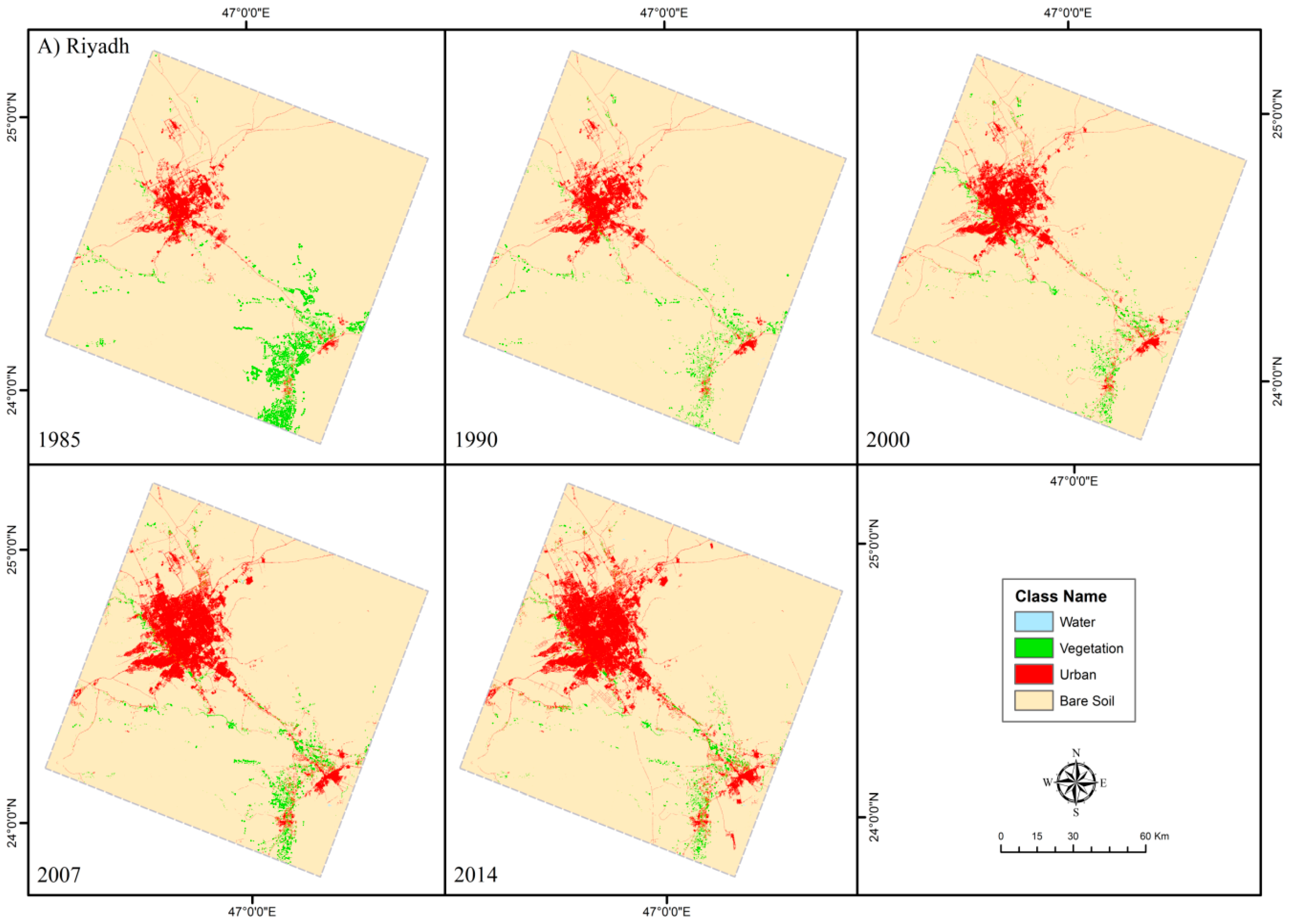
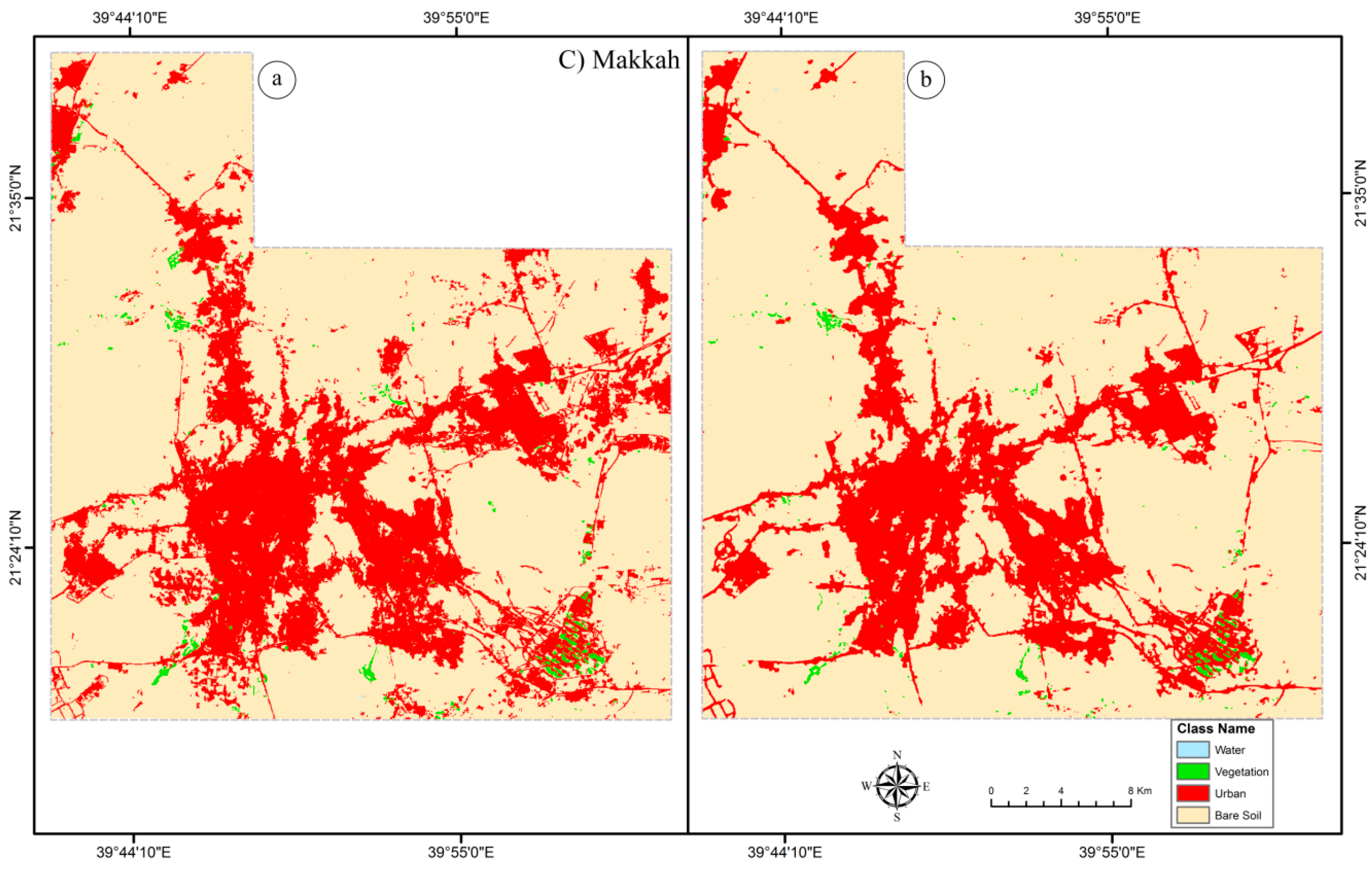
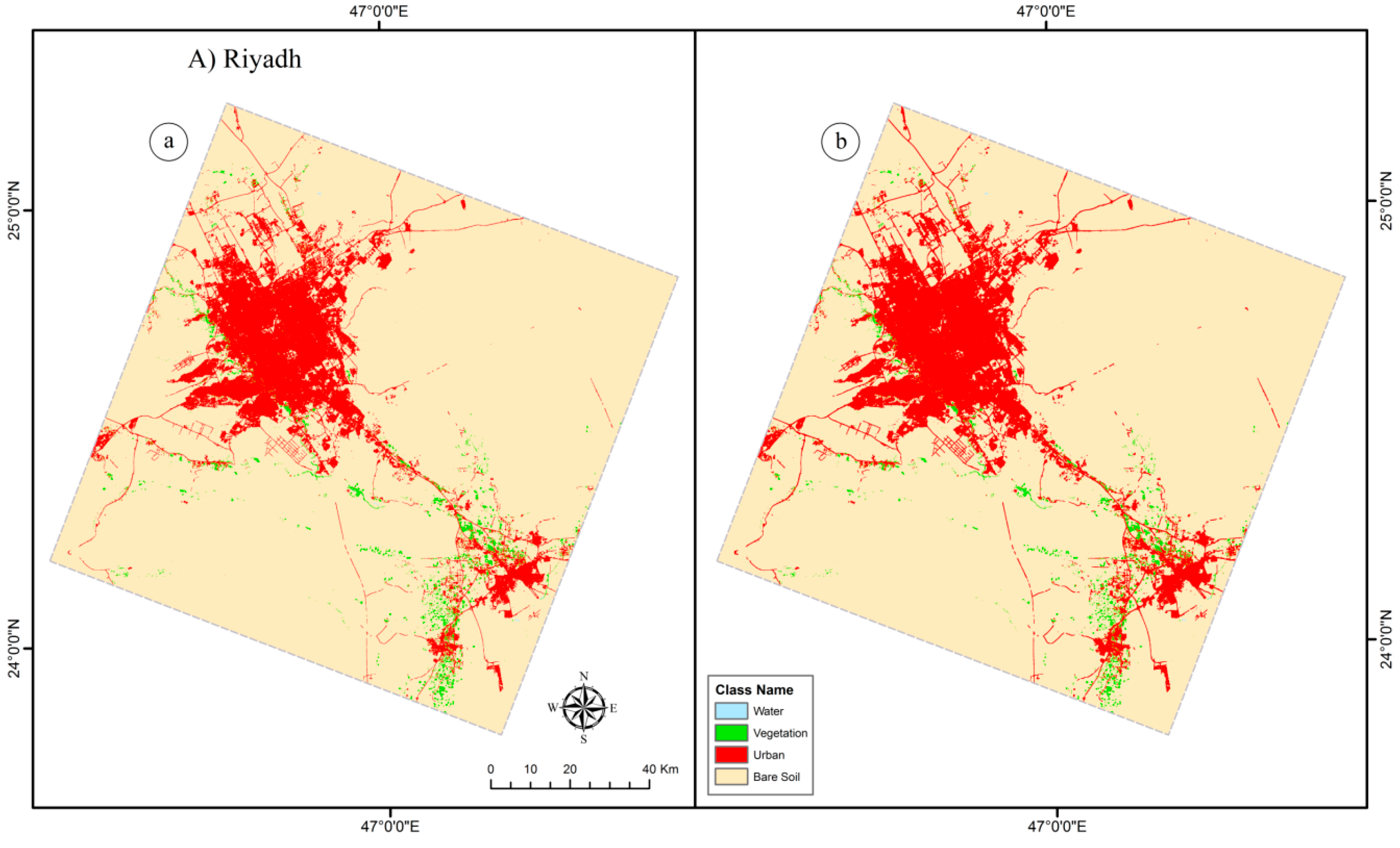
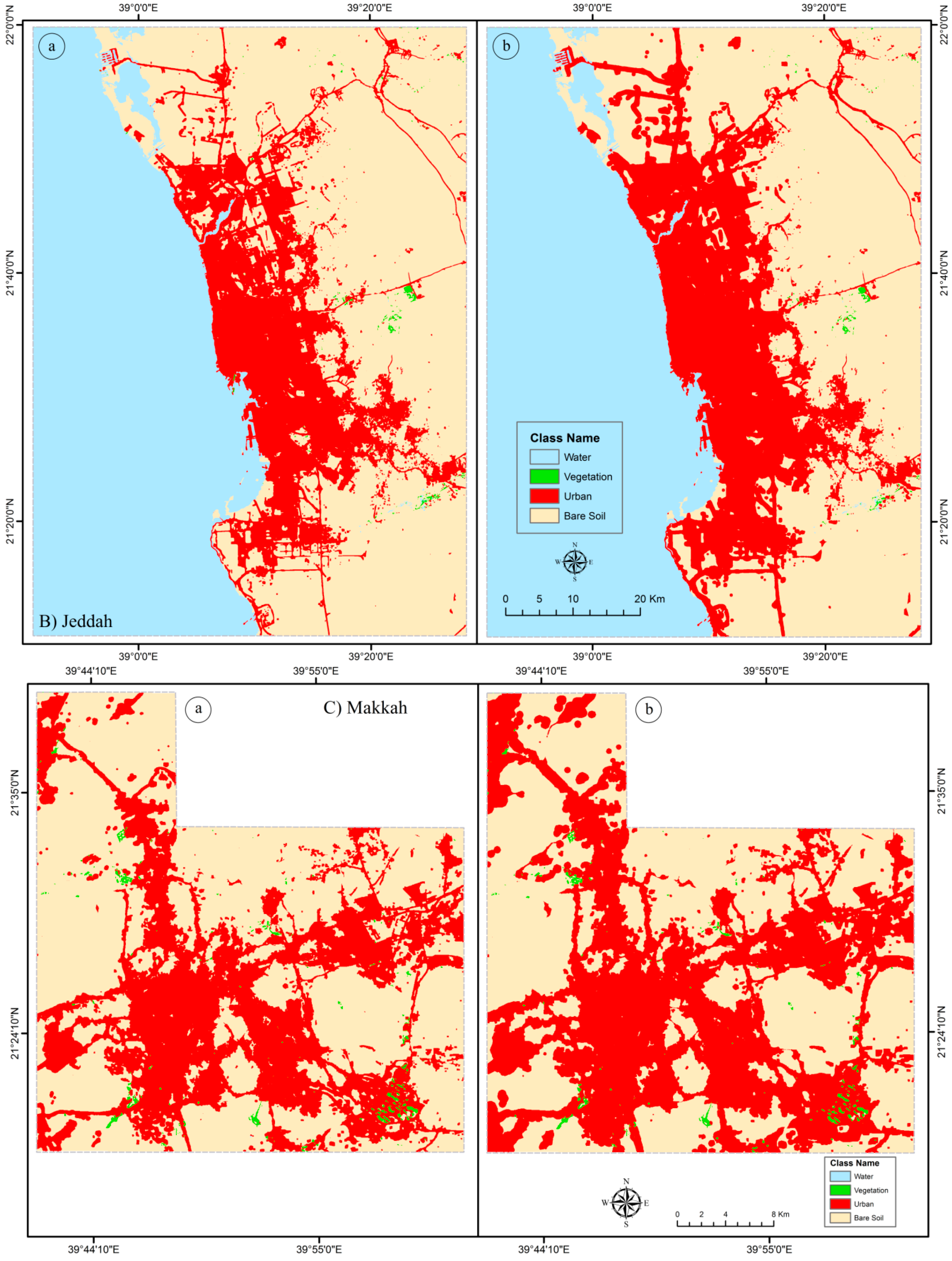
The transition matrix results showed a variation in the conversion from different land cover classes (W, VC and BS) to UA with BS being the most highly converted type of land. This is because BS is the most dominant land type in all the five cities. Although there has been a considerable transition (in terms of area) from VC into UA in almost all of the cities, the conversion of land from VC to BS was higher than the conversion to urbanization. For instance, the transition probability for VC to BS was 93% for the 2000 projection (1985–1990), while the percentage for the transition probability value in terms of UA was only 1%. Similarly, VC is likely to be converted to BS (62%) and to UA (6%) for the 2024 projection (2007–2014). For a desert environment, this is reasonable, as the variations in vegetation abundance is due to erratic rainfall and rising temperatures in these cities. A similar condition applies to W in Riyadh, Makkah and Al-Taif, which showed considerable transition into other land cover uses, except for the sea areas in Jeddah and the Eastern Area.
The results indicate that urban cover was the most developed type of land use among the other land cover features between 1985 and 2014. Similarly in other parts of the world, Dewan and Yamaguchi [71] found that built-up area in Dhaka, Bangladesh was the most expandable land cover type between 1975 and 2003. In Saudi Arabia, Pellikka and Alshaikh [16] showed that urban build-up area was the major changed land cover among other LULC areas between 1984 and 2014 in Al-Baha, Saudi Arabia. The major issue in most of Saudi Arabian cities is that the new development areas are developed wherever vacant lands are available and less expensive. This is due to limitation to apply a master plan that keeps the development within the urban boundaries. As this action may create problems for researchers and planners and lead the growth to be faster than the simulated results using historical data, the simulation results presented in this study should provide the essential information of the future development and provide an overview for the future scenarios in the selected cities.
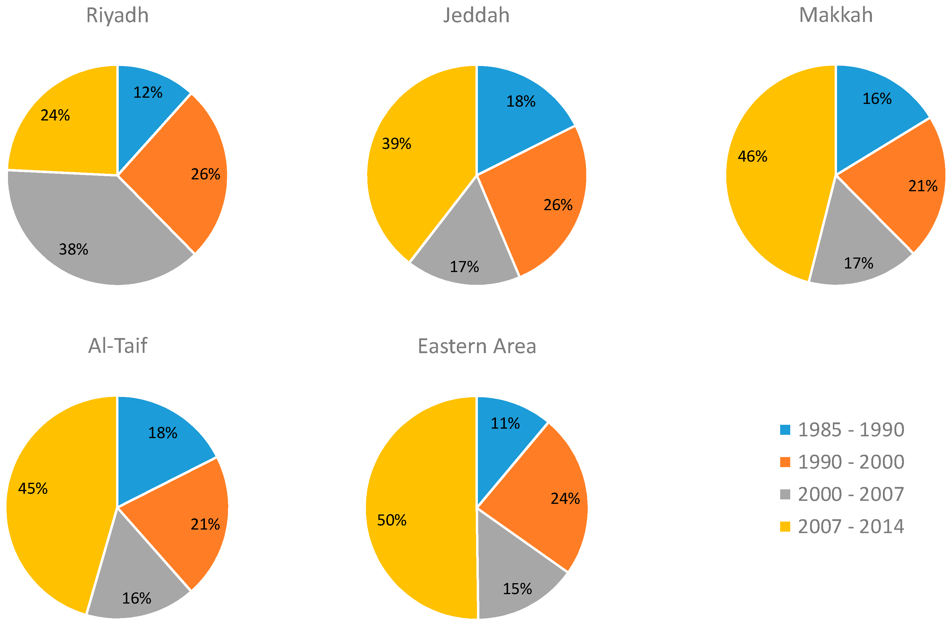
The analysis of urban growth showed variations from 1985 to 2014. For the capital city of Riyadh, high growth took place from 2000 to 2007, which then decreased from 2007 to 2014. In contrast, the growth in Jeddah was relatively similar for all change periods, while the highest increase was observed between 2007 and 2014. Makkah, Al-Taif and Eastern Area also showed massive growth between 2007 and 2014 periods (Figure 8). Figure 8 shows the size of urban growth in percentage for each period between 1985 and 2014. The massive urban growth, potentially in the later years, can be attributed to the increase in the oil price between 2005 and 2014 that allowed increases in the national budget of the country, which was then used for development across the country. The development during this period was directed more towards other cities than the developed cities such as Riyadh. As Figure 8 indicates, 50% of the development of the Eastern Area from 1985 to 2014 was between 2007 and 2014. Just as urban planning has a significant role in past development, it will also contribute to future development. The government now intends to rely on the investment, tourism and industrial sectors by 2020 and into 2030, instead of on oil revenues [72]. Such changes will expand the size of the cities and allow for more development in the near future. The predictions for 2024 and 2034 show an increase in urban growth in all five cities, when most of future development will tend to be close to existing urban areas due to economic benefits [40,73]. With such developments, the local authorities and related sectors will need to join together to provide sustainable development for future urban growth.
The classification of LULC maps was conducted using OBIA technique in this study. The overall accuracies ranged from 82% to 96% in all five cities, which indicates highly robust results to model LULC changes. However, previous studies in Saudi Arabia showed an improvement of the classification accuracy using pixel-based approaches. For example, Rahman [15] used MLC and ISODATA methods to classify urban build-up changes in Al-Khobar, Saudi Arabia and concluded that ISODATA method provided overall accuracy greater than 85%. Similarly, Pellikka and Alshaikh [16] detected LULC changes in Al-Baha, Saudi Arabia using MLC and achieved overall accuracies between 81% and 96%. Thus, compared to these results, both OBIA and traditional pixel-based approaches performed well. This may be due to the medium spatial resolution (e.g., Landsat), where both pixels and objects are nearly similar in scale, which provided approximately similar results.
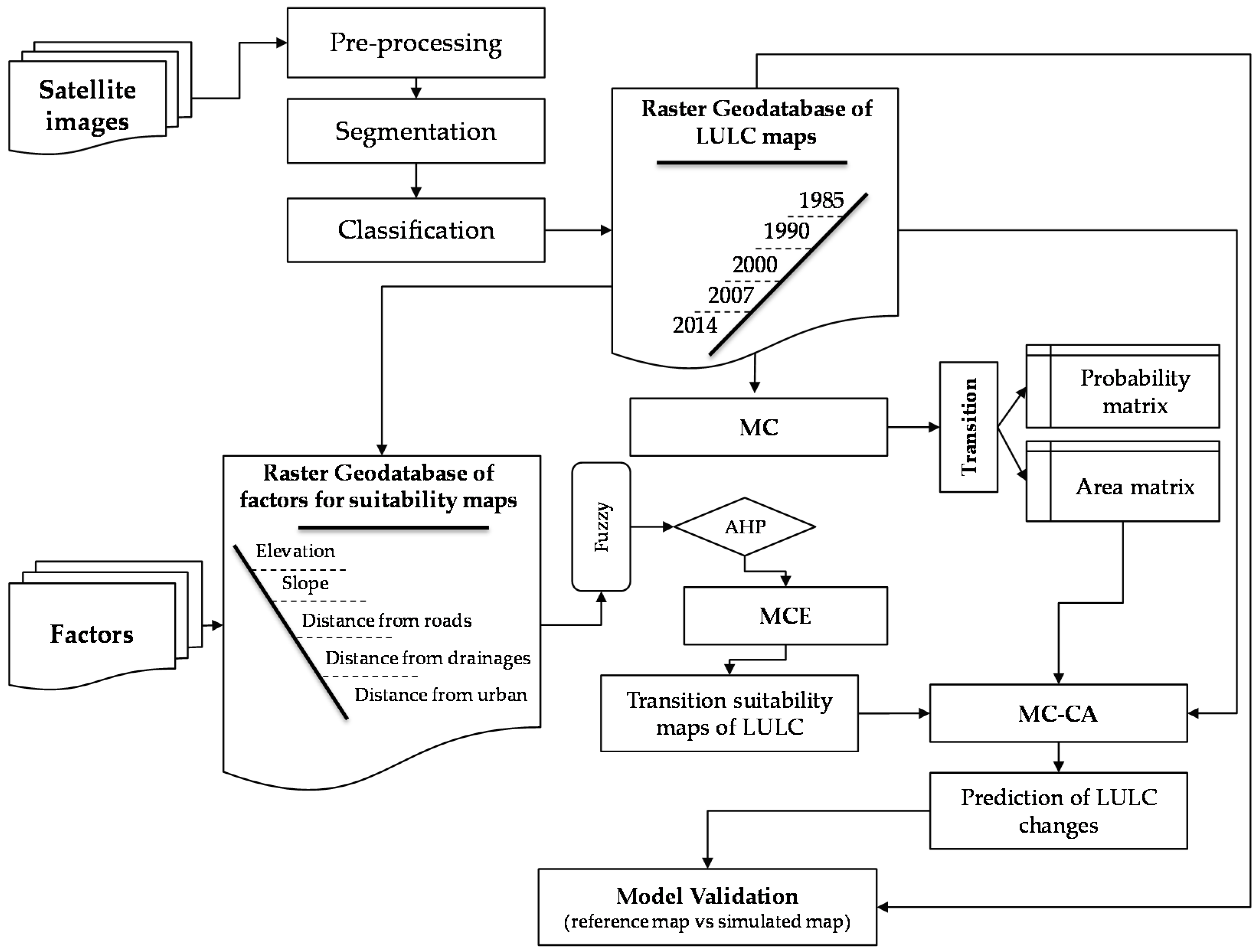
The methodology used in this research provided an opportunity to integrate time-series LULC classifications into MC–CA models. However, the assumptions of MC model that the amount of change observed during the calibration period will remain the same during the entire projection periods is not always true [
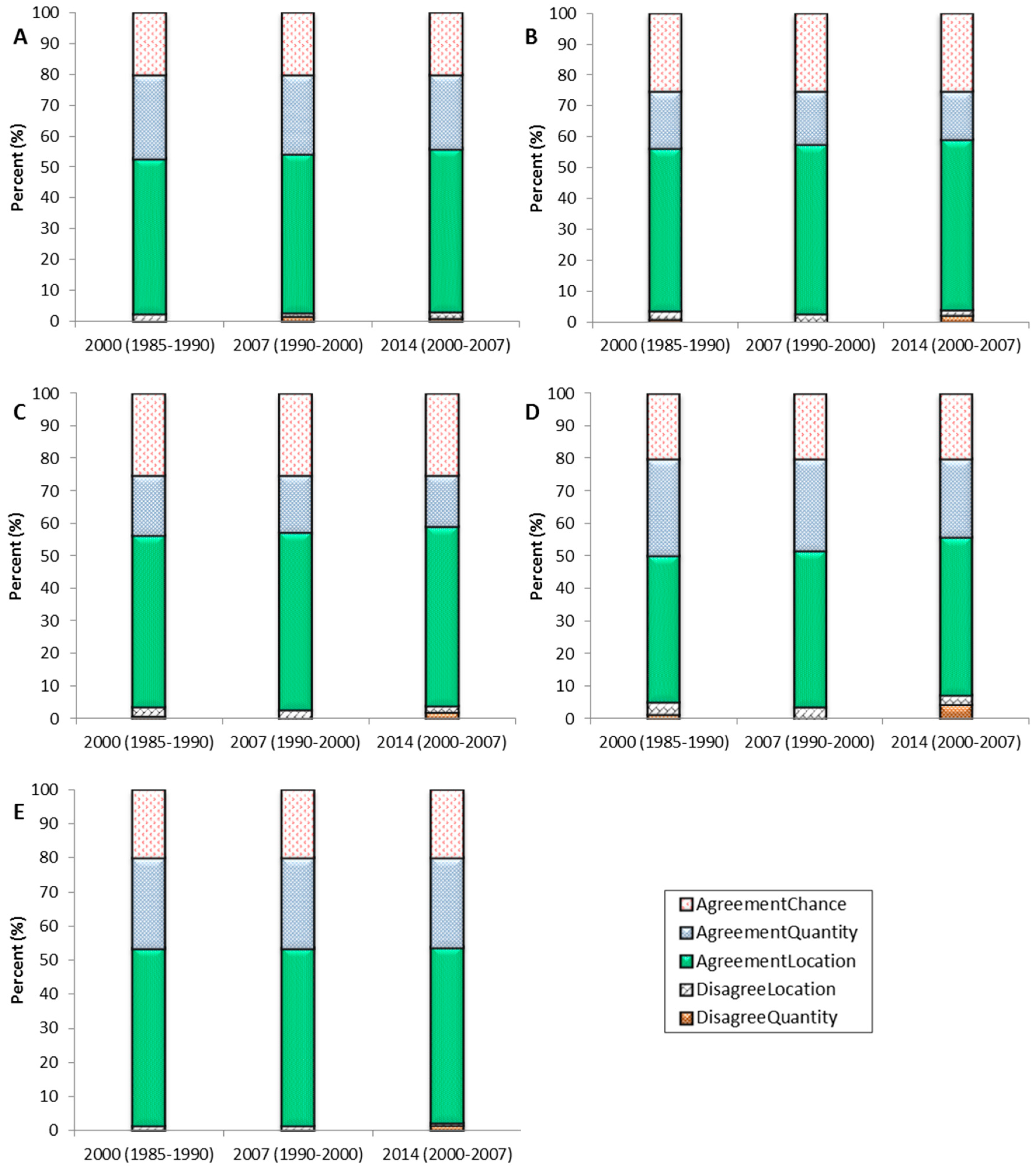
28] because there are other factors that influence the LULC changes and hence impact on the model outcomes. This difficulty is overcome to some extent through the use of CA model that allows us to incorporate other spatial variables to address the neighbourhood effect in the change process. The use of time-series classifications of different change periods has advantage in step-wise model prediction accuracy assessment in terms of urban expansion in the five cities. The MC model used the time-series data to quantify the transition amount and patterns of urban growth, which allowed us to predict urban expansion for the next change period. For example, the 1985 and 1990 LULC classifications were used to predict urban expansion for the year 2000. The simulated change for the year 2000 (predicted) was then compared with the year 2000 classification (reference) to assess the modelling accuracy. The processes were repeated for all the change years. These step-wise evaluations and validation of model outputs in a time series manner allowed achieving higher accuracy in prediction modelling and provided confidence in obtaining nearly accurate future simulations for the years 2024 and 2034. However, there is further scope to improve the model outputs through the inclusion of more variables such as socio-economic and environmental factors as they also contribute significantly towards changes. A subsequent study is planned to include these variables for more accurate predictions.

6. Conclusions

Saudi Arabian cities have faced massive urban growth during the last four decades. Government planning has contributed directly to this expansion and it will continue to support future development. Urban growth is recognized as a key factor that is altering the natural ecosystem and modifying the landscape of the Earth’s surface. Measuring past and present urban growth and modelling future urban growth is essential for understanding its patterns and enabling sustainable development. This study firstly used Landsat TM, ETM+ and OLI satellite images to analyse urban expansion between 1985 and 2014 in five Saudi Arabian cities: Riyadh, Jeddah, Makkah, Al-Taif and the Eastern Area. It then predicted the potential growth in the selected cities for 2024 and 2034 using the MC–CA integrated model based on past land cover classifications. The simulation results showed that urban growth is likely to increase in all five cities during the next 20 years in a similar manner to past growth. The cities are likely to expand near the current growth areas, which may result in complex structures and patterns of urban growth in these cities. Most of the other land cover classes have been converted in the past to urban land use and are likely to convert in a similar way in the future. However, bare soil is the most likely land cover class for conversion into urban areas.
While Remote Sensing data can be effectively used to model dynamic land-cover changes and provide the required information to sufficiently predict future changes, accurate classification of time-series satellite imagery is essential for modelling LULC changes. The simulation of future scenarios is highly dependent on accurate information of historical LULC changes. The error in the LULC classification that is used as a modelling input is a major source for uncertainty in the model’s projections [43,74,75]. In this study, the overall accuracies of LULC change maps were sufficiently high to provide precise simulations for future changes. OBIA and the updating classification approach helped in providing accurate information and reduce the amount of classification time for past land cover changes, especially for large study areas. The future predictions assessed by comparing the simulated and reference maps provided confidence in the model results.
The use of spatial factors such as elevation, slope, distance from drainage, distance from roads and distance from urban determined the neighbourhood suitability for urban growth, which further strengthened the model prediction. However, incorporation of other variables, such as socio-economic and environmental factors, can improve the model predictions for a more detailed interpretation of the future patterns of urban LULC changes. Nevertheless, the prediction results for the future changes produced in this research provide essential information to support the decision-making processes for the planners and local authorities to ensure environmental sustainability and protection of the natural resources of the five cities.

Author Contributions

Abdullah Alqurashi, Lalit Kumar and Priyakant Sinha conceived and designed the experiments; Abdullah Alqurashi performed the experiments; Abdullah Alqurashi and Priyakant Sinha analysed the data; Lalit Kumar contributed reagents/materials/analysis tools; Abdullah Alqurashi wrote the paper; Priyakant Sinha and Lalit Kumar revised the paper.

Conflicts of Interest

The authors declare no conflict of interest.

References

  1. Alberti, M. The effects of urban patterns on ecosystem function. Int. Reg. Sci. Rev. 2005, 28, 168–192. [Google Scholar] [CrossRef]
  2. Guan, D.; Li, H.; Inohae, T.; Su, W.; Nagaie, T.; Hokao, K. Modeling urban land use change by the integration of cellular automaton and Markov model. Ecol. Model. 2011, 222, 3761–3772. [Google Scholar] [CrossRef]
  3. United Nations. World Urbanization Prospects: The 2011 Revision. United Nations, Department of Economic and Social Affairs; Population Division; United Nations: New York, NY, USA, 2012. [Google Scholar]
  4. Grimm, N.B.; Faeth, S.H.; Golubiewski, N.E.; Redman, C.L.; Wu, J.; Bai, X.; Briggs, J.M. Global change and the ecology of cities. Science 2008, 319, 756–760. [Google Scholar] [CrossRef] [PubMed]
  5. Scheffers, B.R.; Paszkowski, C.A. The effects of urbanization on North American amphibian species: Identifying new directions for urban conservation. Urban Ecosyst. 2012, 15, 133–147. [Google Scholar] [CrossRef]
  6. Guderyahn, L.B.; Smithers, A.P.; Mims, M.C. Assessing habitat requirements of pond-breeding amphibians in a highly urbanized landscape: Implications for management. Urban Ecosyst. 2016. [Google Scholar] [CrossRef]
  7. Zang, S.; Wu, C.; Liu, H.; Na, X. Impact of urbanization on natural ecosystem service values: A comparative study. Environ. Monit. Assess. 2011, 179, 575–588. [Google Scholar] [CrossRef] [PubMed]
  8. Rogan, J.; Chen, D. Remote sensing technology for mapping and monitoring land-cover and land-use change. Prog. Plan. 2004, 61, 301–325. [Google Scholar] [CrossRef]
  9. Gómez, C.; White, J.C.; Wulder, M.A. Optical remotely sensed time series data for land cover classification: A review. ISPRS J. Photogramm. Remote Sens. 2016, 116, 55–72. [Google Scholar] [CrossRef]
  10. Chan, J.C.; Chan, K.; Yeh, A.G. Detecting the nature of change in an urban environment: A comparison of machine learning algorithms. Photogramm. Eng. Remote Sens. 2001, 67, 213–226. [Google Scholar]
  11. Schneider, A. Monitoring land cover change in urban and peri-urban areas using dense time stacks of Landsat satellite data and a data mining approach. Remote Sens. Environ. 2012, 124, 689–704. [Google Scholar] [CrossRef]
  12. Bhatta, B. Analysis of urban growth pattern using remote sensing and GIS: A case study of Kolkata, India. Int. J. Remote Sens. 2009, 30, 4733–4746. [Google Scholar] [CrossRef]
  13. Tv, R.; Aithal, B.H.; Sanna, D.D. Insights to urban dynamics through landscape spatial pattern analysis. Int. J. Appl. Earth Obs. Geoinf. 2012, 18, 329–343. [Google Scholar] [CrossRef]
  14. Song, X.; Sexton, J.O.; Huang, C.; Channan, S.; Townshend, J.R. Characterizing the magnitude, timing and duration of urban growth from time series of Landsat-based estimates of impervious cover. Remote Sens. Environ. 2016, 175, 1–13. [Google Scholar] [CrossRef]
  15. Rahman, M. Detection of land use/land cover changes and urban sprawl in Al-Khobar, Saudi Arabia: An analysis of multi-temporal remote sensing data. ISPRS Int. J. Geo-Inf. 2016, 5, 15. [Google Scholar] [CrossRef]
  16. Pellikka, P.; Alshaikh, A.Y. Remote sensing of the decrease of juniper woodlands in the mountains of southwestern Saudi Arabia—Reasons and consequences. Arab. J. Geosci. 2016, 9, 1–12. [Google Scholar] [CrossRef]
  17. Sohl, T.; Sleeter, B. Role of remote sensing for land-use and land-cover change modeling. In Remote Sensing of Land Use and Land Cover; CRC Press: Boca Raton, FL, USA, 2012; pp. 225–240. [Google Scholar]
  18. Singh, A. Review article digital change detection techniques using remotely-sensed data. Int. J. Remote Sens. 1989, 10, 989–1003. [Google Scholar] [CrossRef]
  19. Lu, D.; Mausel, P.; Brondízio, E.; Moran, E. Change detection techniques. Int. J. Remote Sens. 2004, 25, 2365–2401. [Google Scholar] [CrossRef]
  20. Alqurashi, A.F.; Kumar, L. Investigating the use of remote sensing and GIS techniques to detect land use and land cover change: A review. Adv. Remote Sens. 2013, 2, 193–204. [Google Scholar] [CrossRef]
  21. Blaschke, T. Object based image analysis for remote sensing. ISPRS J. Photogramm. Remote Sens. 2010, 65, 2–16. [Google Scholar] [CrossRef]
  22. Myint, S.W.; Gober, P.; Brazel, A.; Grossman-Clarke, S.; Weng, Q. Per-pixel vs. Object-based classification of urban land cover extraction using high spatial resolution imagery. Remote Sens. Environ. 2011, 115, 1145–1161. [Google Scholar] [CrossRef]
  23. Yu, W.; Zhou, W.; Qian, Y.; Yan, J. A new approach for land cover classification and change analysis: Integrating backdating and an object-based method. Remote Sens. Environ. 2016, 177, 37–47. [Google Scholar] [CrossRef]
  24. Hansen, M.C.; Loveland, T.R. A review of large area monitoring of land cover change using Landsat data. Remote Sens. Environ. 2012, 122, 66–74. [Google Scholar] [CrossRef]
  25. Hussain, M.; Chen, D.; Cheng, A.; Wei, H.; Stanley, D. Change detection from remotely sensed images: From pixel-based to object-based approaches. ISPRS J. Photogramm. Remote Sens. 2013, 80, 91–106. [Google Scholar] [CrossRef]
  26. Taubenböck, H.; Esch, T.; Felbier, A.; Wiesner, M.; Roth, A.; Dech, S. Monitoring urbanization in mega cities from space. Remote Sens. Environ. 2012, 117, 162–176. [Google Scholar] [CrossRef]
  27. Platt, R.V.; Ogra, M.V.; Badola, R.; Hussain, S.A. Conservation-induced resettlement as a driver of land cover change in India: An object-based trend analysis. Appl. Geogr. 2016, 69, 75–86. [Google Scholar] [CrossRef]
  28. Mas, J.; Kolb, M.; Paegelow, M.; Camacho Olmedo, M.T.; Houet, T. Inductive pattern-based land use/cover change models: A comparison of four software packages. Environ. Model. Softw. 2014, 51, 94–111. [Google Scholar] [CrossRef] [Green Version]
  29. Ahmed, B.; Kamruzzaman, M.; Zhu, X.; Rahman, M.; Choi, K. Simulating land cover changes and their impacts on land surface temperature in Dhaka, Bangladesh. Remote Sens. 2013, 5, 5969–5998. [Google Scholar] [CrossRef] [Green Version]
  30. Liao, J.; Tang, L.; Shao, G.; Su, X.; Chen, D.; Xu, T. Incorporation of extended neighborhood mechanisms and its impact on urban land-use cellular automata simulations. Environ. Model. Softw. 2016, 75, 163–175. [Google Scholar] [CrossRef]
  31. Wu, F. Calibration of stochastic cellular automata: The application to rural-urban land conversions. Int. J. Geogr. Inf. Sci. 2002, 16, 795–818. [Google Scholar] [CrossRef]
  32. Hu, Z.; Lo, C.P. Modeling urban growth in Atlanta using logistic regression. Comput. Environ. Urban Syst. 2007, 31, 667–688. [Google Scholar] [CrossRef]
  33. Gong, J.; Liu, Y.; Xia, B.; Zhao, G. Urban ecological security assessment and forecasting, based on a cellular automata model: A case study of Guangzhou, China. Ecol. Model. 2009, 220, 3612–3620. [Google Scholar] [CrossRef]
  34. Luo, J.; Wei, Y.H.D. Modeling spatial variations of urban growth patterns in Chinese cities: The case of Nanjing. Landsc. Urban Plan. 2009, 91, 51–64. [Google Scholar] [CrossRef]
  35. Myint, S.W.; Jain, J.; Lukinbeal, C.; Lara-Valencia, F. Simulating urban growth on the US-Mexico border: Nogales, Arizona, and Nogales, Sonora. Can. J. Remote Sens. 2010, 36, 166–184. [Google Scholar] [CrossRef]
  36. Aljoufie, M.; Zuidgeest, M.; Brussel, M.; van Vliet, J.; van Maarseveen, M. A cellular automata-based land use and transport interaction model applied to Jeddah, Saudi Arabia. Landsc. Urban Plan. 2013, 112, 89–99. [Google Scholar] [CrossRef]
  37. Shafizadeh M., H.; Helbich, M. Spatiotemporal variability of urban growth factors: A global and local perspective on the megacity of Mumbai. Int. J. Appl. Earth Obs. Geoinf. 2015, 35, 187–198. [Google Scholar] [CrossRef]
  38. Alqurashi, A.F.; Kumar, L.; Al-Ghamdi, K.A. Spatiotemporal modeling of urban growth predictions based on driving force factors in five Saudi Arabian cities. ISPRS Int. J. Geo-Inf. 2016, 5, 139. [Google Scholar] [CrossRef]
  39. Ahmed, B.; Ahmed, R. Modeling urban land cover growth dynamics using multi‑temporal satellite images: A case study of Dhaka, Bangladesh. ISPRS Int. J. Geo-Inf. 2012, 1, 3–31. [Google Scholar] [CrossRef]
  40. Shafizadeh M., H.; Helbich, M. Spatiotemporal urbanization processes in the megacity of Mumbai, India: A Markov chains-cellular automata urban growth model. Appl. Geogr. 2013, 40, 140–149. [Google Scholar] [CrossRef]
  41. Ozturk, D. Urban growth simulation of Atakum (Samsun, Turkey) using cellular automata-Markov chain and multi-layer perceptron-markov chain models. Remote Sens. 2015, 7, 5918–5950. [Google Scholar] [CrossRef]
  42. Weng, Q. Land use change analysis in the Zhujiang Delta of China using satellite remote rensing, GIS and stochastic modelling. J. Environ. Manag. 2002, 64, 273–284. [Google Scholar] [CrossRef]
  43. Sinha, P.; Kumar, L. Markov land cover change modeling using pairs of time-series satellite images. Photogramm. Eng. Remote Sens. 2013, 79, 1037–1051. [Google Scholar] [CrossRef]
  44. Lo, C.; Yang, X. Drivers of land-use/land-cover changes and dynamic modeling for the Atlanta, Georgia metropolitan area. Photogramm. Eng. Remote Sens. 2002, 68, 1073–1082. [Google Scholar]
  45. White, R.; Engelen, G. Cellular automata as the basis of integrated dynamic regional modelling. Environ. Plan. B Plan. Des. 1997, 24, 235–246. [Google Scholar] [CrossRef]
  46. He, C.; Okada, N.; Zhang, Q.; Shi, P.; Li, J. Modelling dynamic urban expansion processes incorporating a potential model with cellular automata. Landsc. Urban Plan. 2008, 86, 79–91. [Google Scholar] [CrossRef]
  47. Alqurashi, A.F.; Kumar, L. Land use and land cover change detection in the Saudi Arabian desert cities of Makkah and Al-Taif using satellite data. Adv. Remote Sens. 2014, 3, 106–119. [Google Scholar] [CrossRef]
  48. Al-Ahmadi, K.; See, L.; Heppenstall, A.; Hogg, J. Calibration of a fuzzy cellular automata model of urban dynamics in Saudi Arabia. Ecol. Complex. 2009, 6, 80–101. [Google Scholar] [CrossRef]
  49. Aljoufie, M. Toward integrated land use and transport planning in fast-growing cities: The case of Jeddah, Saudi Arabia. Habitat Int. 2014, 41, 205–215. [Google Scholar] [CrossRef]
  50. Baatz, M.; Schäpe, A. Multiresolution segmentation: An optimization approach for high quality multi-scale image segmentation. Angew. Geogr. Inf. 2000, 58, 12–23. [Google Scholar]
  51. Mathieu, R.; Aryal, J.; Chong, A. Object-based classification of IKONOS imagery for mapping large-scale vegetation communities in urban areas. Sensors 2007, 7, 2860–2880. [Google Scholar] [CrossRef]
  52. Pu, R.; Landry, S.; Yu, Q. Object-based urban detailed land cover classification with high spatial resolution IKONOS imagery. Int. J. Remote Sens. 2011, 32, 3285–3308. [Google Scholar] [CrossRef]
  53. Zhou, W.; Troy, A. An object-oriented approach for analysing and characterizing urban landscape at the parcel level. Int. J. Remote Sens. 2008, 29, 3119–3135. [Google Scholar] [CrossRef]
  54. Zhou, W.; Troy, A.; Grove, M. Object-based land cover classification and change analysis in the Baltimore metropolitan area using multitemporal high resolution remote sensing data. Sensors 2008, 8, 1613–1636. [Google Scholar] [CrossRef]
  55. Foody, G.M. Thematic map comparison: Evaluating the statistical significance of differences in classification accuracy. Photogramm. Eng. Remote Sens. 2004, 70, 627–633. [Google Scholar] [CrossRef]
  56. Foody, G.M. Harshness in image classification accuracy assessment. Int. J. Remote Sens. 2008, 29, 3137–3158. [Google Scholar] [CrossRef]
  57. Sinha, P.; Kumar, L. Independent two-step thresholding of binary images in inter-annual land cover change/no-change identification. ISPRS J. Photogramm. Remote Sens. 2013, 81, 31–43. [Google Scholar] [CrossRef]
  58. Sinha, P.; Kumar, L.; Reid, N. Rank-based methods for selection of landscape metrics for land cover pattern change detection. Remote Sens. 2016, 8. [Google Scholar] [CrossRef]
  59. López, E.; Bocco, G.; Mendoza, M.; Duhau, E. Predicting land-cover and land-use change in the urban fringe: A case in Morelia city, Mexico. Landsc. Urban Plan. 2001, 55, 271–285. [Google Scholar] [CrossRef]
  60. Eastman, J.R. Idrisi Andes Guide to GIS and Image Processing; Clark University: Worcester, UK, 2006. [Google Scholar]
  61. United States Geological Survey (USGS), SRTM Data. Avaliable online: http://earthexplorer.usgs.gov/ (accessed on 16 May 2016).
  62. Mirza, M.; Dawod, G.; Al-Ghamdi, K. Accuracy and relevance of digital elevation models for geomatics applications-a case study of Makkah municipality, Saudi Arabia. Int. J. Geomat. Geosci. 2011, 1, 803–812. [Google Scholar]
  63. Eastman, J.R. Multi-criteria evaluation and GIS. Geogr. Inf. Syst. 1999, 1, 493–502. [Google Scholar]
  64. Pontius, R.G. Quantification error versus location error in comparison of categorical maps. Photogramm. Eng. Remote Sens. 2000, 66, 1011–1016. [Google Scholar]
  65. Pontius, R.G. Statistical methods to partition effects of quantity and location during comparison of categorical maps at multiple resolutions. Photogramm. Eng. Remote Sens. 2002, 68, 1041–1050. [Google Scholar]
  66. Pontius, R.G.; Millones, M. Death to Kappa: Birth of quantity disagreement and allocation disagreement for accuracy assessment. Int. J. Remote Sens. 2011, 32, 4407–4429. [Google Scholar] [CrossRef]
  67. Pontius, R.G.; Suedmeyer, B. Components of agreement between categorical maps at multiple resolutions. Remote Sens. GIS Accuracy Assess. 2004, 233–251. [Google Scholar] [CrossRef]
  68. Selim, M.E. Environmental security in the Arab World. In Facing Global Environmental Change: Environmental, Human, Energy, Food, Health and Water Security Concepts; Brauch, H.G., Spring, Ú.O., Grin, J., Mesjasz, C., Kameri-Mbote, P., Behera, N.C., Chourou, B., Krummenacher, H., Eds.; Springer: Berlin/Heidelberg, Germany, 2009; pp. 843–853. [Google Scholar]
  69. Rahman, M.; Aldosary, A.; Nahiduzzaman, K.; Reza, I. Vulnerability of flash flooding in Riyadh, Saudi Arabia. Natl. Hazards 2016, 1–24. [Google Scholar] [CrossRef]
  70. Alamri, Y. Rains and floods in Saudi Arabia. Crying of the sky or of the people? Saudi Med. J. 2011, 32, 311–313. [Google Scholar] [PubMed]
  71. Dewan, A.; Yamaguchi, Y. Land use and land cover change in greater Dhaka, Bangladesh: Using remote sensing to promote sustainable urbanization. Appl. Geogr. 2009, 29, 390–401. [Google Scholar] [CrossRef]
  72. Saudi-Arabia-Vision-2030. Vision 2030, the Kingdom of Saudi Arabia; The Council of Economic and Development Affairs: Riyadh, Saudi Arabia, 2016. [Google Scholar]
  73. McDonald, J.F. Fundamentals of Urban Economics; Prentice Hall: Upper Saddle River, NJ, USA, 1997. [Google Scholar]
  74. Fang, S.; Wente, S.; Gertner, Z.G.; Wang, G.; Anderson, A. Uncertainty analysis of predicted disturbance from off-road vehicular traffic in complex landscapes at fort hood. Environ. Manag. 2002, 30, 199–208. [Google Scholar] [CrossRef] [PubMed]
  75. Carmel, Y.; Dean, D.J. Performance of a spatio-temporal error model for raster datasets under complex error patterns. Int. J. Remote Sens. 2004, 25, 5283–5296. [Google Scholar] [CrossRef]
Figure 1. Geographical locations with the estimation of population of 2015 (in millions) of the selected study sites in Saudi Arabia.
Remotesensing 08 00838 g001
Figure 2. Flowchart of the research methodology.
Remotesensing 08 00838 g002
Figure 3. An example of factors used to create the suitability maps in Jeddah. The continuous suitability scale ranges from 255 (most suitable) to 0 (least suitable).
Remotesensing 08 00838 g003
Figure 4. Spatial distribution of LULC changes between 1985 and 2014 in three cities: (A) Riyadh; (B) Jeddah; (C) Makkah.
Remotesensing 08 00838 g004aRemotesensing 08 00838 g004b
Figure 5. Validation of the MC–CA integrated model for allocation and quantity agreement for (A) Riyadh; (B) Jeddah; (C) Makkah; (D) Al-Taif; and (E) the Eastern Area simulations.
Remotesensing 08 00838 g005
Figure 6. A comparison between the reference LULC change map (a) and the simulation map of LULC changes (b) in 2014 for (A) Riyadh; (B) Jeddah; (C) Makkah.
Remotesensing 08 00838 g006aRemotesensing 08 00838 g006b
Figure 7. A prediction of the future land cover changes in (a) 2024 and (b) 2034 for (A) Riyadh; (B) Jeddah; (C) Makkah.
Remotesensing 08 00838 g007aRemotesensing 08 00838 g007b
Figure 8. The differences in urban growth in percentage between the observation dates.
Remotesensing 08 00838 g008
Table 1. The 2015 population and importance of the five cities.
CityPopulation (M)Importance
Riyadh6.7Capital city
Jeddah4Commercial hub nationally
Makkah2Pilgrimage and holy places
Al-Taif1.1Tourism sector
Eastern Area2.8Oil production industry
Table 2. Information of Landsat data used to classify land cover changes.
CitySensorPath/RowDate
Eastern AreaTM164/41-42(15 June 1985), (31 July 1990)
ETM+(6 July 2000), (6 July 2007)
OLI(2 August 2014)
RiyadhTM165-166/43(13–20 January 1985), (14–15 August 1990), (18–25 August 2000)
ETM+(29–20 July 2007)
OLI(9–16 August 2014)
Makkah & Al-TaifTM169/45(30 March 1985), (27 August 1990)
ETM+(6 August 2000), (5 August 2007)
OLI(5 August 2014)
JeddahTM170/45(9 June 1985), (11 September 1990)
ETM+(1 November 2000), (17 August 2007)
OLI(29 September 2014)
Table 3. Description of LULC classes.
ClassDefinition
WaterSeas, lakes, dames and stream surfaces
VegetationNatural vegetation, crop fields and green spaces
Bare SoilSand desert, bare rocky and mountains
UrbanBuilt-up lands, human-constructed elements and transportation
Table 4. List of overall accuracies and Kappa statistics of the classified images.
ImageOverall AccuracyKappa Coefficient
1985199020002007201419851990200020072014
Riyadh87.594.590.888.992.80.820.920.870.850.90
Jeddah92.490.185.686.294.90.880.830.750.770.92
Makkah87.285.987.486.783.80.770.800.820.810.73
Al-Taif89.189.688.984.581.90.810.840.830.770.73
Eastern Area96.292.388.689.289.30.940.870.820.840.83
Table 5. Markov transition probability matrices.
Riyadh Jeddah Makkah Al-Taif Eastern Area
1990 1990 1990 1990 1990
LULCWVCBSUA LULCWVCBSUA LULCWVCBSUA LULCWVCBSUA LULCWVCBSUA
1985W0.290.040.660.011985W1.000.000.000.001985W0.000.010.740.251985W0.160.460.360.021985W0.990.000.010.00
VC0.000.060.930.01VC0.010.160.420.40VC0.000.070.860.07VC0.000.250.680.07VC0.010.580.300.11
BS0.000.010.980.02BS0.010.000.940.05BS0.000.000.940.06BS0.000.010.930.06BS0.050.010.910.04
UA0.000.000.001.00UA0.000.000.001.00UA0.000.000.001.00UA0.000.000.001.00UA0.000.000.001.00
2000 2000 2000 2000 2000
LULCWVCBSUA LULCWVCBSUA LULCWVCBSUA LULCWVCBSUA LULCWVCBSUA
1990W0.550.300.130.021990W0.990.000.010.001990W0.000.000.001.001990W0.200.170.570.061990W0.990.000.010.00
VC0.000.460.520.02VC0.010.680.160.15VC0.000.390.530.07VC0.000.720.230.04VC0.000.630.270.11
BS0.000.010.980.01BS0.000.010.960.03BS0.000.010.970.03BS0.000.010.970.03BS0.000.000.970.03
UA0.000.000.001.00UA0.000.000.001.00UA0.000.000.001.00UA0.000.000.001.00UA0.000.000.001.00
2007 2007 2007 2007 2007
LULCWVCBSUA LULCWVCBSUA LULCWVCBSUA LULCWVCBSUA LULCWVCBSUA
2000W0.480.110.370.052000W1.000.000.000.002000W0.000.001.000.002000W0.000.070.930.002000W0.990.000.000.00
VC0.000.580.390.03VC0.000.240.620.14VC0.000.430.440.14VC0.000.470.490.04VC0.000.610.290.09
BS0.000.010.960.03BS0.000.000.970.03BS0.000.000.960.03BS0.000.010.960.03BS0.010.010.950.03
UA0.000.000.001.00UA0.000.000.001.00UA0.000.000.001.00UA0.000.000.001.00UA0.000.000.001.00
2014 2014 2014 2014 2014
LULCWVCBSUA LULCWVCBSUA LULCWVCBSUA LULCWVCBSUA LULCWVCBSUA
2007W0.240.010.620.142007W0.990.000.010.002007W0.000.000.610.392007W0.000.000.320.682007W0.990.000.010.01
VC0.000.320.620.06VC0.030.110.570.30VC0.000.460.450.09VC0.000.600.260.13VC0.030.380.120.47
BS0.000.010.970.02BS0.000.000.900.09BS0.000.010.860.14BS0.000.020.860.12BS0.010.010.850.13
UA0.000.000.001.00UA0.000.000.001.00UA0.000.000.001.00UA0.000.000.001.00UA0.000.000.001.00
2024 2024 2024 2024 2024
LULCWVCBSUA LULCWVCBSUA LULCWVCBSUA LULCWVCBSUA LULCWVCBSUA
2014W0.860.000.000.142014W1.000.000.000.002014W0.600.000.000.402014W0.320.000.000.682014W0.990.000.000.01
VC0.000.940.000.06VC0.000.700.000.30VC0.000.910.000.09VC0.000.870.000.13VC0.000.530.000.47
BS0.000.000.980.02BS0.000.000.910.09BS0.000.000.860.14BS0.000.000.880.12BS0.000.000.920.08
UA0.000.000.001.00UA0.000.000.001.00UA0.000.000.001.00UA0.000.000.001.00UA0.000.000.001.00
Table 6. Absolute urban growth (in ha) between 1985 and 2014 and for the expected growth for the years 2024 and 2034.
YearRiyadhJeddahMakkahAl-TaifEastern Area
Area (ha)(%)Area (ha)(%)Area (ha)(%)Area (ha)(%)Area (ha)(%)
198550,604.022.923,321.937.810184.930.15173.354.733,234.427.7
199062,174.341.632,132.440.813,252.930.38003.342.342,444.746.3
200088,041.843.145,242.718.617,264.517.811,390.322.662,106.620.0
2007125,958.319.153,677.337.020,345.742.613,969.552.674,543.355.9
2014150,050.022.373,526.235.729,020.737.721,320.044.3116,203.928.7
2024183,503.917.899,761.023.939,963.523.630,755.726.9149,542.816.1
2034216,110.9 123,583.5 49,393.7 39,026.0 173,605.5

