Article

A Comparison of Different Regression Algorithms for Downscaling Monthly Satellite-Based Precipitation over North China

1
State Key Laboratory of Resources and Environmental Information System, Institute of Geographic Sciences and Natural Resources Research, Chinese Academy of Sciences, Beijing 100101, China
2
University of Chinese Academy of Sciences, Beijing 100049, China
3
Jiangsu Center for Collaborative Innovation in Geographical Information Resource Development and Application, Nanjing 210023, China
*
Author to whom correspondence should be addressed.
Remote Sens. 2016, 8(10), 835; https://doi.org/10.3390/rs8100835
Submission received: 7 June 2016 / Revised: 25 September 2016 / Accepted: 8 October 2016 / Published: 12 October 2016

Abstract

:
Environmental monitoring of Earth from space has provided invaluable information for understanding land–atmosphere water and energy exchanges. However, the use of satellite-based precipitation observations in hydrologic and environmental applications is often limited by their coarse spatial resolutions. In this study, we propose a downscaling approach based on precipitation–land surface characteristics. Daytime land surface temperature, nighttime land surface temperature, and day–night land surface temperature differences were introduced as variables in addition to the Normalized Difference Vegetation Index (NDVI), the Digital Elevation Model (DEM), and geolocation (longitude, latitude). Four machine learning regression algorithms, the classification and regression tree (CART), the k-nearest neighbors (k-NN), the support vector machine (SVM), and random forests (RF), were implemented to downscale monthly TRMM 3B43 V7 precipitation data from 25 km to 1 km over North China for the purpose of comparison of algorithm performance. The downscaled results were validated based on observations from meteorological stations and were also compared to a previous downscaling algorithm. According to the validation results, the RF-based model produced the results with the highest accuracy. It was followed by SVM, CART, and k-NN, but the accuracy of the downscaled results using SVM relied greatly on residual correction. The downscaled results were well correlated with the observations during the year, but the accuracies were relatively lower in July to September. Downscaling errors increase as monthly total precipitation increases, but the RF model was less affected by this proportional effect between errors and observation compared with the other algorithms. The variable importances of the land surface temperature (LST) feature variables were higher than those of NDVI, which indicates the significance of considering the precipitation–land surface temperature relationship when downscaling TRMM 3B43 V7 precipitation data.

Graphical Abstract

1. Introduction

Attaining accurate and fine spatial resolution precipitation data is very important for understanding land surface processes and global climate change. Observations from meteorological stations and rain gauges have long temporal series records and are important means of acquiring precipitation data; however, the acquisition of precipitation observations over mountainous and underdeveloped areas remains a great challenge due to the sparse rain gauge network [1,2,3]. Ground weather radar systems can also provide spatial precipitation information but validation of ground radar rainfall products and the high uncertainties are major challenges for broad utilization in hydrologic application [4,5]. Moreover, weather radar systems also have a limited range and are generally aimed at monitoring of extreme rainfall events over limited time spans, making their use less suitable for long-term and broad area assessments [6]. The development of satellite sensors and remote sensing technology has resulted in multiple sources of precipitation datasets [7,8,9,10,11,12,13,14,15,16,17,18] that provide more reliable estimations of precipitation over un-gauged areas compared with various interpolation methods. A series of precipitation datasets at both regional and global scales have been developed by research institutions and government organizations, for example, the Global Precipitation Climatology Project (GPCP) [9], the Global Satellite Mapping of Precipitation (GSMaP) project [19], the Climate Hazards Group InfraRed Precipitation with Station data (CHIRPS) [20,21] and the Tropical Rainfall Measuring Mission (TRMM) [10]. These precipitation datasets have been widely used in various kinds of studies. However, the spatial resolution of these data is too coarse when specific to local basin and region scales [6,22].
Downscaling techniques have provided an efficient approach for acquiring fine-resolution data from a dataset having coarse spatial resolution, and great efforts have been made to advance downscaling algorithms of satellite-based precipitation datasets. Immerzeel et al. [6] proposed an algorithm for downscaling Tropical Rainfall Measuring Mission (TRMM) datasets using the exponential regression function between the precipitation and the Normalized Difference Vegetation Index (NDVI). Jia et al. [22] improved the algorithm by using a multiple linear regression model and introduced both NDVI and digital elevation model (DEM) as independent variables. Chen et al. and Xu et al. constructed a geographically weighted regression model based on the assumption that the rainfall–geospatial factors relationship varies spatially but is similar within a region [23,24]. Shi et al. [25] developed a downscaling algorithm by introducing a machine learning algorithm termed Random Forests (RF) to detect the complex precipitation–NDVI and precipitation–DEM relationships, and their validation results indicated that the RF-based downscaling model outperformed the linear regression and exponential regression models.
Due to the spatial variation and complex nonlinear relationship between precipitation and surface properties, it is difficult to map precipitation with fine resolution from satellite-based precipitation datasets using traditional statistical regression algorithms, especially over regions with heterogeneous environments. Compared with traditional statistical algorithms, machine learning techniques have been reported to be excellent in dealing with complex nonlinear problems. Although a large number of algorithms have been developed and applied for downscaling of satellite-based precipitation data and improvements in accuracy have been reported, it is difficult to find a comparison of the performance of the different algorithms. This is particularly true for machine learning algorithms, as many of these have been introduced into the field of remote sensing within the past 10 years [26,27]. In this study, we implemented four machine learning regression algorithms, classification and regression tree (CART), k-nearest neighbors, random forests (RF), and support vector machine (SVM), for downscaling of TRMM 3B43 V7 data in order to gain a better understanding of the performance of each algorithm.
In addition, we introduced land surface temperature as a factor for enhancing the precipitation–land surface characteristics relationships when downscaling precipitation data, considering that the satellite precipitation datasets over regions with no relationship with NDVI and DEM could not be downscaled with these algorithms [23]. Considerable relationships between land surface temperature and precipitation have been observed and detected [28]. Precipitation can change the local land surface temperature during both daytime and nighttime; it is cooler when it is raining, and heat waves often accompany drought [29]. We used land surface temperature at both daytime and nighttime, day–night temperature difference, vegetation index (NDVI), DEM, and geolocations (longitude and latitude) as input independent variables for the downscaling of the monthly TRMM 3B43 V7 precipitation dataset and conducted a case study over North China for the years 2003, 2006, and 2009.

2. Study Area and Data Resources
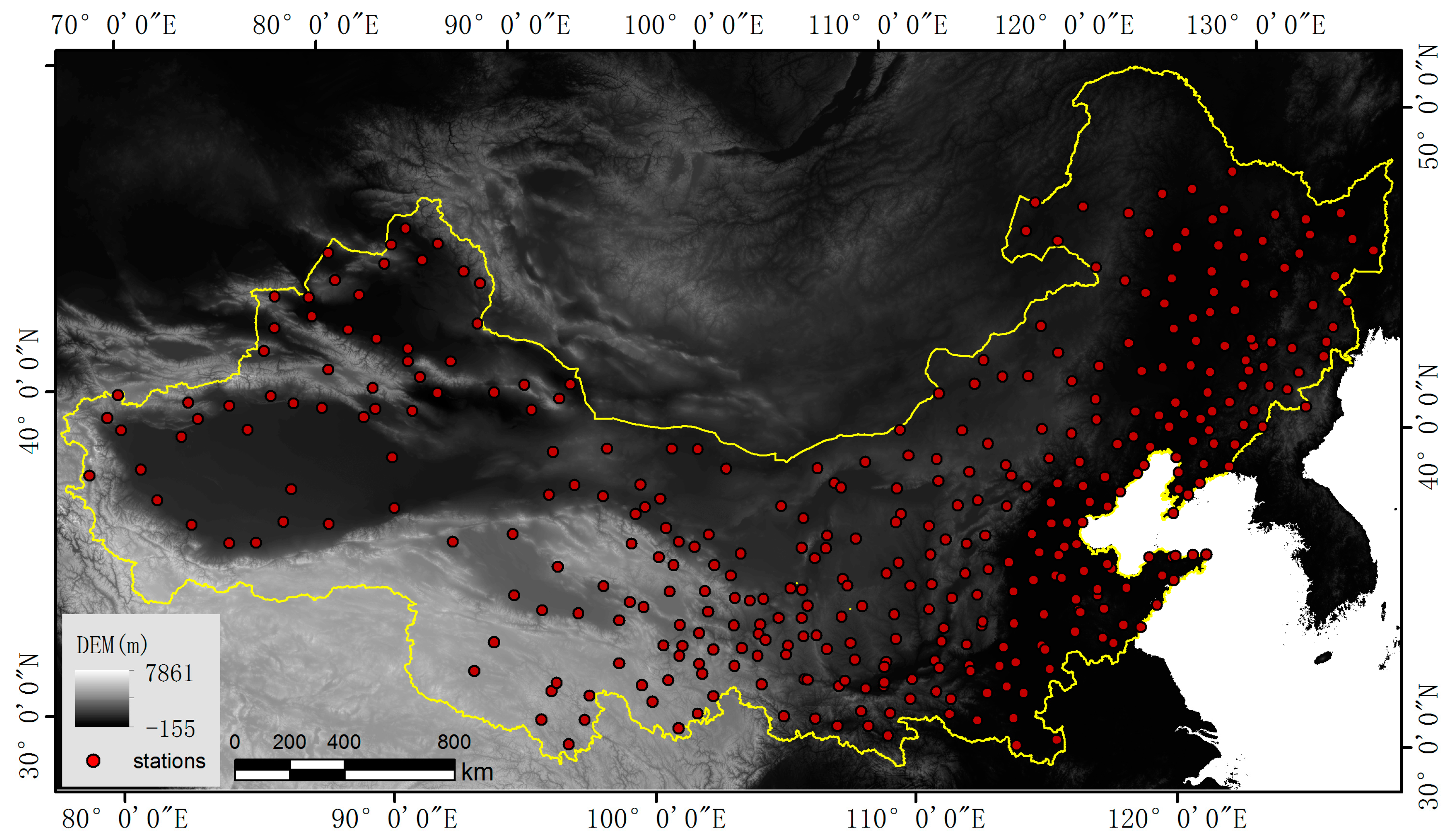
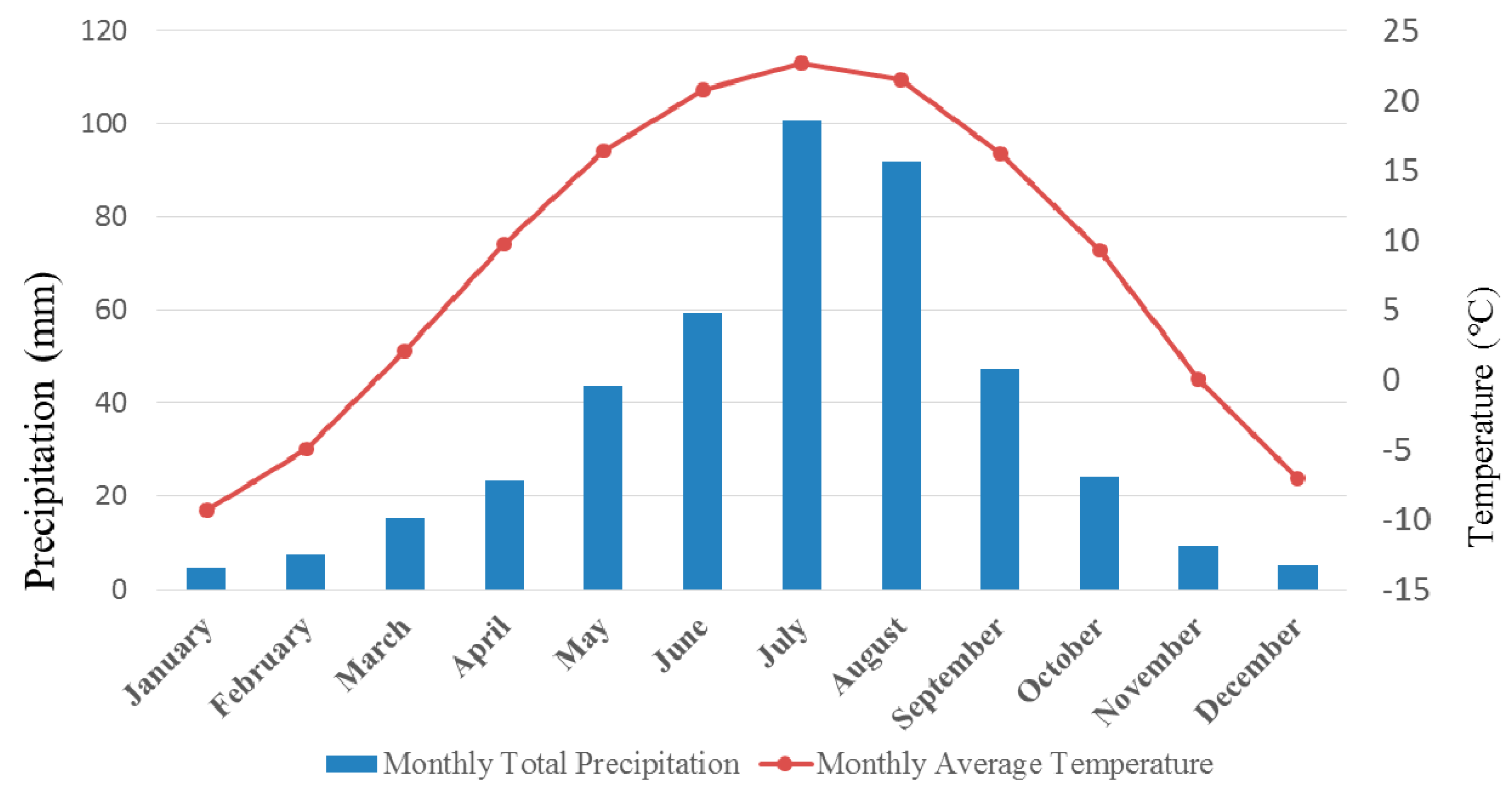
2.1. Study Area

North China was selected for the case study. The study area, with a total area of 5,643,270 km2 between 31°23′N–53°34′N and 73°00′E–135°05′E, includes 13 provinces and two municipalities. The natural environment is very heterogeneous over North China. The topography of North China varies greatly, from west to east, from mountainous regions and plateau regions to inhospitable desert zones and flat, fertile plains [30] (Figure 1). There are 378 meteorological stations throughout the area and the spatial distribution is uneven (the observation records data were provided by National Meteorological Information Center) [31]. As depicted in Figure 1, the distribution of stations in the study area is dense in the east and relatively sparse in the west. Problems arise as to how to map precipitation with high spatial resolution for the study of ecology and hydrology in North China. The climate of China is dominated mainly by dry seasons and wet monsoons [30,32], which lead to pronounced precipitation and temperature differences between winter and summer [33] (Figure 2). The distribution of precipitation during the year is also uneven and the seasonal variability is significant. According to Figure 2, precipitation increases from January to July and decreases from July to December. The coldest month is January, and the warmest is July. Preliminary research revealed a close relationship between precipitation and other environmental elements over North China. Most parts of North China are typical of arid and semi-arid areas; the dry/wet state of the land surface is affected by precipitation hydrological processes [34]. The distribution of vegetation and the vegetation condition are highly correlated to precipitation [35,36]. Thus, the land surface temperature (LST) and NDVI are effective indicators of precipitation [37]. Therefore, it is feasible to develop a spatial downscaling algorithm for low-resolution satellite-based precipitation datasets based on NDVI, DEM, and land surface temperature.

2.2. Data Resources

The Tropical Rainfall Measuring Mission (TRMM), a joint mission of NASA and the Japan Aerospace Exploration Agency, was launched in 1997 to study rainfall for weather and climate research. TRMM is a research satellite designed to improve our understanding of the distribution and the variability of the precipitation over the tropical and subtropical regions of the Earth, and it has provided much needed information about rainfall and its associated release of heat [10]. The TRMM 3B43 product provides monthly precipitation data at a spatial resolution of 0.25° × 0.25° for the area of 50°N–50°S. Version 7 of the TRMM 3B43 product (termed TRMM 3B43 V7), from January to December of 2003, 2006, and 2009, the periods used in this study, was downloaded from the National Aeronautics and Space Administration (NASA) Precipitation Measurement Missions (PMM) website [38]. Then, the original TRMM 3B43 V7 data were re-projected to the Albers Conical Equal Area projection and resampled to a resolution of 25 km using the nearest neighbor resampling algorithm during the re-projection.
Monthly NDVI (MOD13A3) and land surface temperature acquired by Terra (MOD11A1) were downloaded from the NASA Land Processes Distributed Active Archive Center (LP DAAC) [39]. These products, provided at 1 km spatial resolution in the sinusoidal projection, were re-projected to the Albers Conical Equal Area projection, and the nearest neighbor resampling algorithm was used to resample MODIS NDVI images to maintain the pixel size of 1 km × 1 km. MOD11A1 is comprised of daytime and nighttime land surface temperatures (LSTs) at daily interval. Monthly average LSTs were calculated by averaging the daily LSTs of each month.
The DEM data used in this study were from the NASA Shuttle Radar Topographic Mission (SRTM) [40]. DEM data of two spatial resolutions, 30 m and 90 m, were available. Considering the spatial scales of this study, we downloaded the DEM data with a spatial resolution of 90 m and then re-sampled these data to 1 km by averaging the values of all pixels within each 1-km pixel.

3. Methods

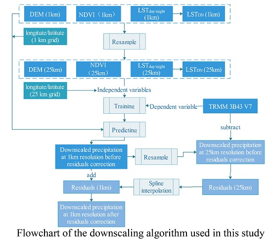
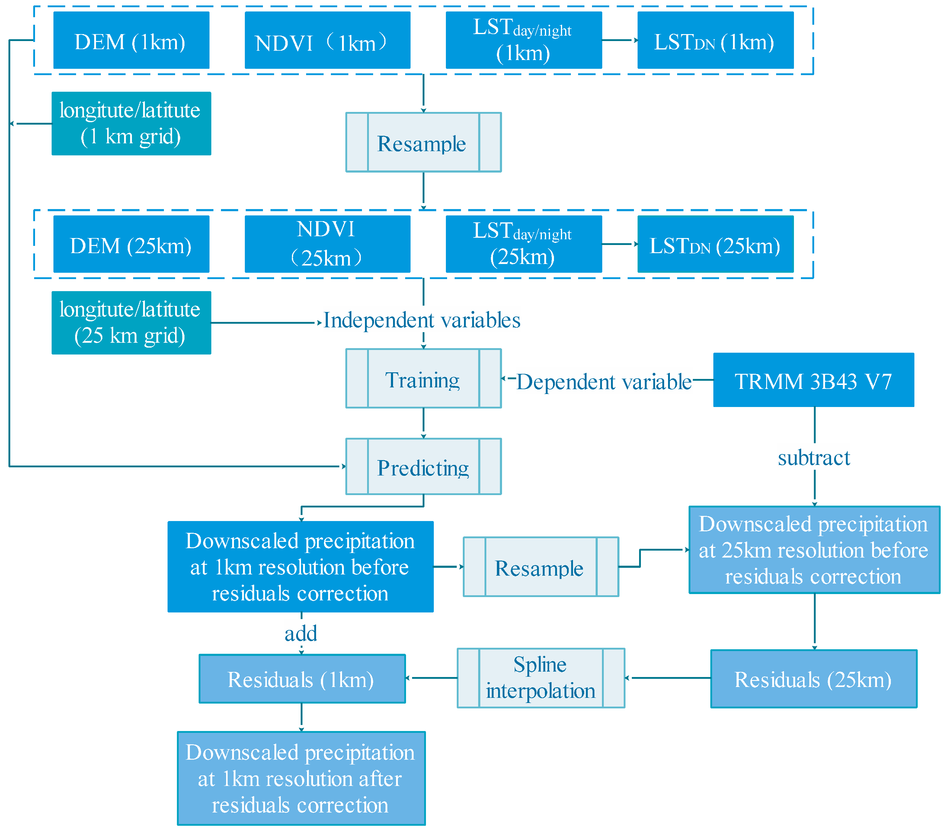
3.1. Downscaling Algorithm

The downscaling method is based on two assumptions: (1) the precipitation has a spatial relationship with the land surface characteristics, and this relationship can be addressed by machine learning regression models; and (2) the models established at low spatial resolution can also be used to predict the precipitation at fine resolution with the higher resolution land surface characteristics dataset. In this study, we used five land surface characteristics and geolocations as independent variables, NDVI, DEM, daytime land surface temperature (termed LSTday), nighttime land surface temperature (termed LSTnight), day–night land surface temperature difference (termed LSTDN), and longitude and latitude, to downscale the TRMM 3B43 V7 precipitation data. Regression algorithms were implemented to detect the possible relationships between precipitation and the independent variables. The process of the downscaling model used in this study is described below, and a flowchart of the method is shown in Figure 3:
(1)
For regions with snow, water bodies, and desert-covered areas, NDVI values are usually constantly under 0.0. To eliminate the influences of snow and water bodies, the threshold of NDVI <0.0 was used to distinguish and remove snow and water body pixels from the original monthly NDVI images.
(2)
LSTDN was calculated by subtracting LSTnight from LSTday. Additionally, NDVI1km, DEM1km, LSTday-1km, LSTnight-1km, LSTDN-1km were re-sampled to a resolution of 25 km using an averaging method, and the geographical coordinates of the center of each 25 km × 25 km grid were extracted.
(3)
The relationships between the re-sampled independent variables and the TRMM 3B43 V7 precipitation data were established using the regression algorithms.
(4)
Fine spatial resolution (1 km) variables and the geolocations were input into the model established in step (3), and downscaled precipitation of 1 km resolution (termed PRE1km) was achieved.
(5)
Residual correction is an essential step for a downscaling method based on statistical algorithms, and it can correct the precipitation that cannot be predicted by the models. The PRE1km were re-sampled to 25 km using the simple averaging method. Then, the residuals of the models were calculated by subtracting the re-sampled PRE1km from the original TRMM data.
(6)
The residuals were interpolated to a spatial resolution of 1 km using a simple spline tension interpolator [6,22] and then added back to the PRE1km. Thus, corrected downscaled precipitation results (PREC-1km) were obtained.

3.2. Regression Algorithms

3.2.1. Machine Learning Algorithms

We experimented with four types of machine learning regression algorithms: classification and regression trees (CART), k-nearest neighbors (k-NN), support vector machine (SVM), and random forests (RF).
CART is a commonly used machine learning algorithm [41]. Its basic concept is to construct a tree-like graph or model of decisions and their possible consequences by generating relatively homogeneous subgroups by recursively partitioning the training dataset to the maximum variance between groups of independent variables and dependent variables. In each of the terminal nodes of the tree, a simple and accurate model is built to explain the relationship of independent and dependent variables [42].
The k-NN method is a non-parametric method used for classification and regression [43]. For k-NN regression, the property value for the object is defined by the average values of its k nearest neighbors; Euclidean distance, a common distance metric for continuous variables, is used to define the neighbors.
Support vector machine (SVM) is an outstanding machine learning algorithm for classification and regression problems and has been applied successfully in various fields, such as soil moisture estimation [44], impervious surface estimation [45], and biophysical parameter estimation from remote sensing data [46]. The original SVM algorithm was invented by Vapnik and co-workers in the early 1990s for classification problems and then was extended to the case of regression [47,48]. The basic concept of the SVM algorithm is derived from an optimization theory that uses a hyperplane to classify the input variables into an m-dimensional feature space with maximal margin. The maximal margin is derived by solving a constrained quadratic problem:
Maximiza W ( α ) = i = 1 n α i 1 2 i = 1 n j = 1 n α i α j y i y j K ( x i , x j )
Subject to   { i = 1 n α i y i = 0   a n d   0 α i   C   f o r   i = 1 , 2 , n }
where x i R d are the training sample vectors and K ( x i , x j ) is the kernel function.
f ( x , ω ) = j = 1 m ω j g j ( x ) + b ,
where g j ( x ) , j = 1, 2,…m denotes a set of nonlinear transformations and b is the “bias” term.
Random forests (RF), a non-parametric and ensemble learning algorithm for regression and classification, has been increasingly applied because it yields high accuracy and is robust to outliers [49]. RF, which was proposed by Breiman [50], is a combination of tree predictors such that each tree depends on the values of a randomly chosen subset of input variable vectors sampled independently and with the same distribution for all trees in the forests [50]. The tree predictor is based on the classification and regression trees (CART) algorithm [42]. The RF regression algorithm process can be described briefly as follows:
(1)
The ntree (number of trees) samples sets are randomly drawn from the original training sample set with replacement. Each sample set is a bootstrap sample, and the elements that are not included in the bootstrap are termed “out-of-bag data” (OOB) for that bootstrap sample.
(2)
For each bootstrap sample, an un-pruned regression tree is grown with the modification that a random subset of the variables, from which the best variables are split, is selected at each node.
(3)
Predictions for new samples can be made by averaging the predictions from all the individual regression trees:
f = 1 N   i = 1 N f i ( x ) ,
where N is the number of trees and f i ( x ) is the prediction from each individual regression tree.
The ranking of variable importance is an important issue in the RF algorithm. During the fitting process, the prediction error for each out-of-bag (OOB) sample is recorded and averaged over the forest. To measure the importance of the i-th variable, the values of that variable are permuted while the values of other independent variables are kept unchanged. Then, the OOB error is again computed on this perturbed dataset. The importance score for the i-th variable is computed by averaging the difference in the out-of-bag (OOB) error before and after the permutation over all trees. These variable importance values are then used to rank the independent variables in terms of their contribution to the regression model.
The four machine learning regression algorithms were all from easily accessible sources. These selected algorithms are openly accessible and easy to use, and they are clearly documented elsewhere. Sources of the codes were implemented in scikit-learn, which is a Python package integrating a wide range of state-of-the-art machine learning algorithms for medium-scale supervised and unsupervised problems [51]. Most algorithms require certain parameterizations. Although the choice of an optimal parameter set is desirable, it is extremely difficult to do so as the application conditions vary widely from one environment to another and from one data type to another. In practice, we designed experiments to cover a majority of the parameter combinations for each algorithm [41,42,43,50,51,52,53,54] (Table 1), and a grid search algorithm was implemented to find the optimal parameters. The grid search is an approach implemented in scikit-learn [51] for specialized, efficient parameter search strategies. It exhaustively generates candidates from a grid of parameter values specified with the parameter combinations and fits these on a dataset. All of the possible combinations of parameter values are evaluated and the best combination is retained.

3.2.2. Multiple Linear Regression (MLR) Algorithm

The multiple linear regression (MLR) model proposed by Jia et al. [22] was also used for downscaling the TRMM 3B43 V7 data. Jia et al. [22] used a multiple linear regression model to fit the relationships of TRMM precipitation with NDVI and elevation, downscaling the TRMM precipitation data to a fine spatial resolution. In this study, we constructed the multiple linear regression model with NDVI, DEM, LSTs, and geolocations as independent variables:
P = a 1 N D V I + a 2 D E M + a 3 L S T d a y + a 4 L S T n i g h t + a 5 L S T D N + a 6 L a t + a 7 L o n + c
where a 1 , a 2 , …, a n are the slopes of each independent variable and c is the intercept of the regression function.

4. Results and Analysis

4.1. Performance of the Different Algorithms

Table 2 shows the average coefficients of determination (R2), mean absolute error (MAE), and root mean square error (RMSE) estimated by each model for each month. It should be noted a grid search was conducted to find the optimal parameters for each month, and a stepwise regression was used to establish the MLR model. On average, RF produced the highest R2 (R2 = 0.989) and the lowest MAE (MAE = 1.5 mm) and RMSE (RMSE = 2.6 mm), followed the CART, k-NN, and SVM; MLR produced the lowest R2 and the highest MAE and RMSE.

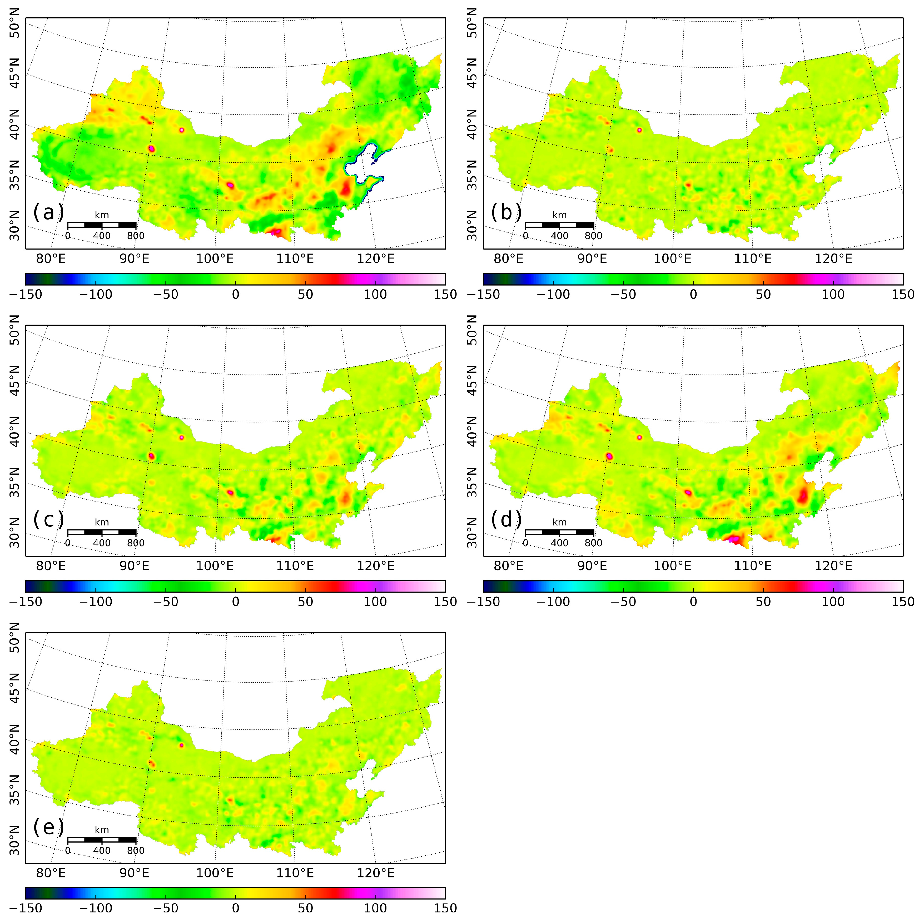
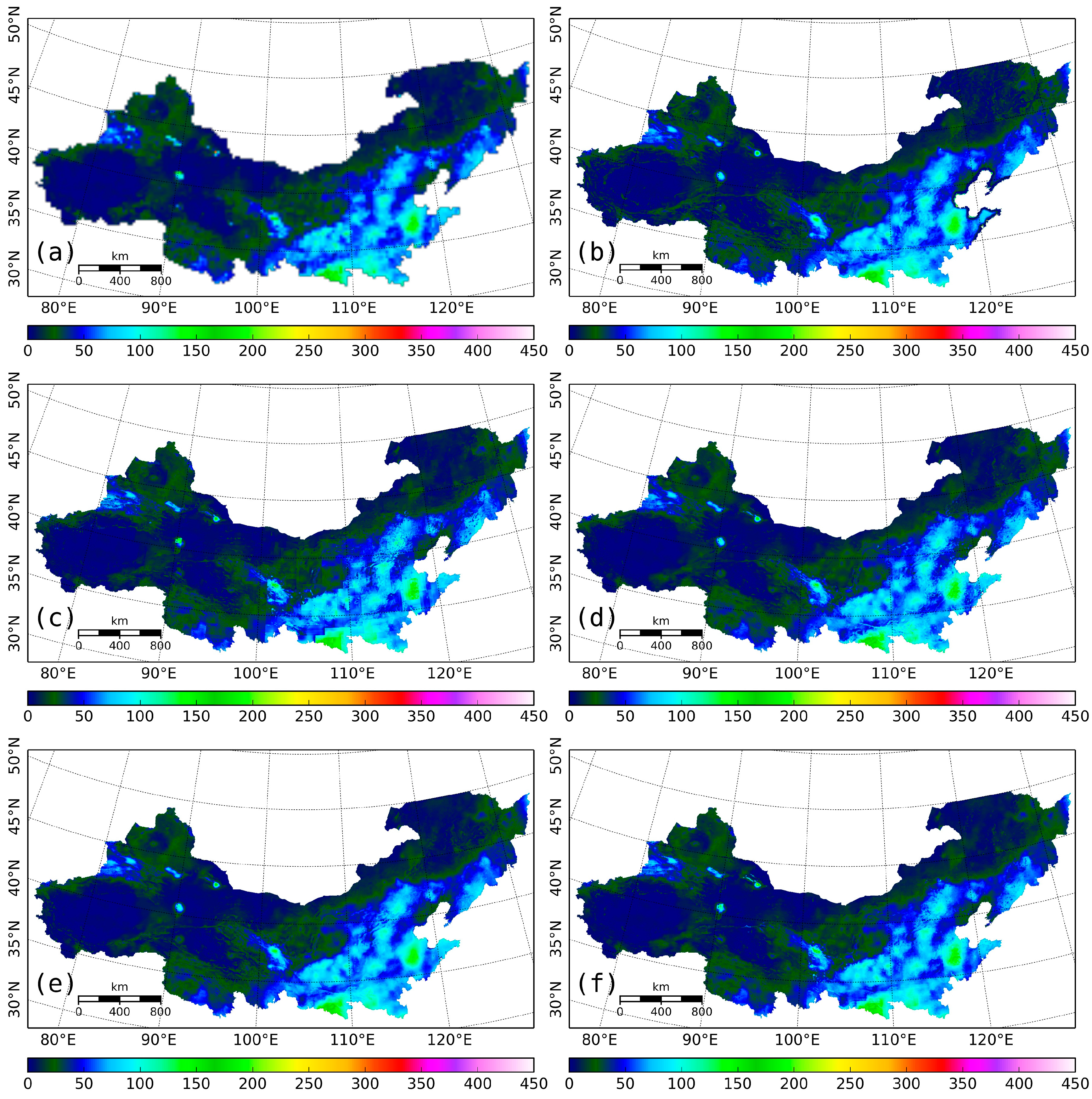
4.2. Downscaled Results

Figure 4 shows the downscaled results using the five regression algorithms before residual correction over the North China area in May 2006, with the TRMM 3B43 V7 also displayed (Figure 4a). The results of MLR and SVM before residual correction show significantly different spatial distribution patterns compared to that of the original TRMM 3B43 V7, whereas the downscaled results of RF, CART, and k-NN have spatial distribution patterns similar to that of TRMM 3B43 V7.
The residuals were calculated using the approach described above. Figure 5 shows the residuals interpolated by the spline tension interpolator. The spatial distribution of the residual of the MLR model indicates that it tends to underestimate TRMM 3B43 V7 precipitation over the southern and eastern parts of the study area. The residual of SVM presents a distribution pattern similar to that of MLR. In contrast, CART and RF present much lower residuals and irregular spatial distribution patterns.
Figure 6 shows the downscaled precipitation data after residual correction. Compared to the downscaled results without residual correction (Figure 4), the downscaled results of the MLR and SVM models after residual correction are more likely to show a spatial distribution pattern similar to that of the original TRMM 3B43 V7. In contrast, the downscaled results of CART and RF after residual correction show little difference compared to the results before residual correction.

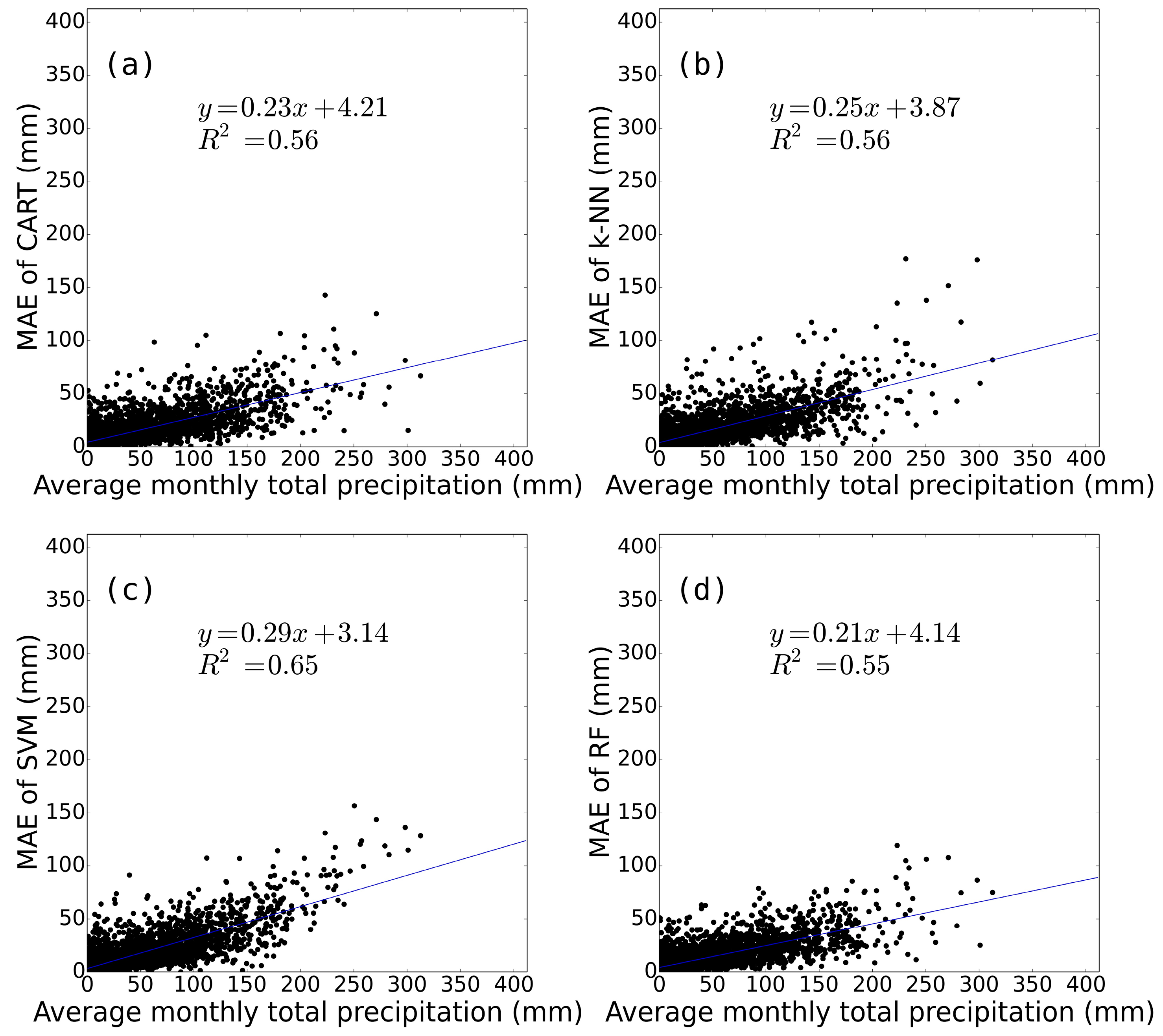
4.3. Validation and Error Analysis

The downscaled results of each algorithm were validated using the observation records from 378 rain gauges over the area of North China for the years of 2003, 2006, and 2009. The downscaled results before and after residual correction were all validated to assess the effects of residual correction. Table 3 shows the coefficients of determination (R2), mean absolute error (MAE), and root mean square error (RMSE) of each algorithm before residual correction. According to the validation results, the RF algorithm produced the results with the highest accuracy (R2 = 0.736, MAE = 11.6 mm, RMSE = 16.5 mm) compared to the other four algorithms. The CART algorithm ranked second with R2 = 0.677, MAE = 12.6 mm, and RMSE = 18.5 mm, followed the k-NN and SVM, while MLR produced the results having the worst accuracy.
Table 4 shows the accuracy of each algorithm after residual correction. In general, RF was also the best-performing algorithm based on the validation results after residual correction. However, significant improvements of the accuracy of SVM and k-NN were produced by the residual correction. SVM had the second-best accuracy, attaining values of R2, MAE, and RMSE close to those of RF, followed by CART, k-NN, and MLR, respectively. For each individual month during January to December, the downscaled results were well correlated with the observations, but the accuracies of the downscaled results were relatively lower during July to September.
To investigate the relationship between the estimation errors and the precipitation observations, we calculated the averaged MAE of the downscaled results for each station and the average precipitation observations of the stations. Here, for investigation of the performance of the downscaling algorithms, we used the downscaled results before residual correction to exclude the influence of the residual correction. Figure 7 shows scatter plots between averaged MAE and the average precipitation observations for the models. In general, the estimation errors tend to be positively related to the average precipitation, and the MAEs increased linearly as the average precipitation increased. The MAE of the k-NN model increased at a rate of 2.4 mm/10 mm (R2 = 0.56), and the MAE increase rate of the SVM model was 3.0 mm/10 mm (R2 = 0.65). The analogous rates of the CART and RF models were 2.5 mm/10 mm (R2 = 0.56) and 2.1 mm/10 mm (R2 = 0.55). These results indicate that errors increase as monthly total precipitation increases and that the rate of increase of RF was the lowest among the four machine learning algorithms.

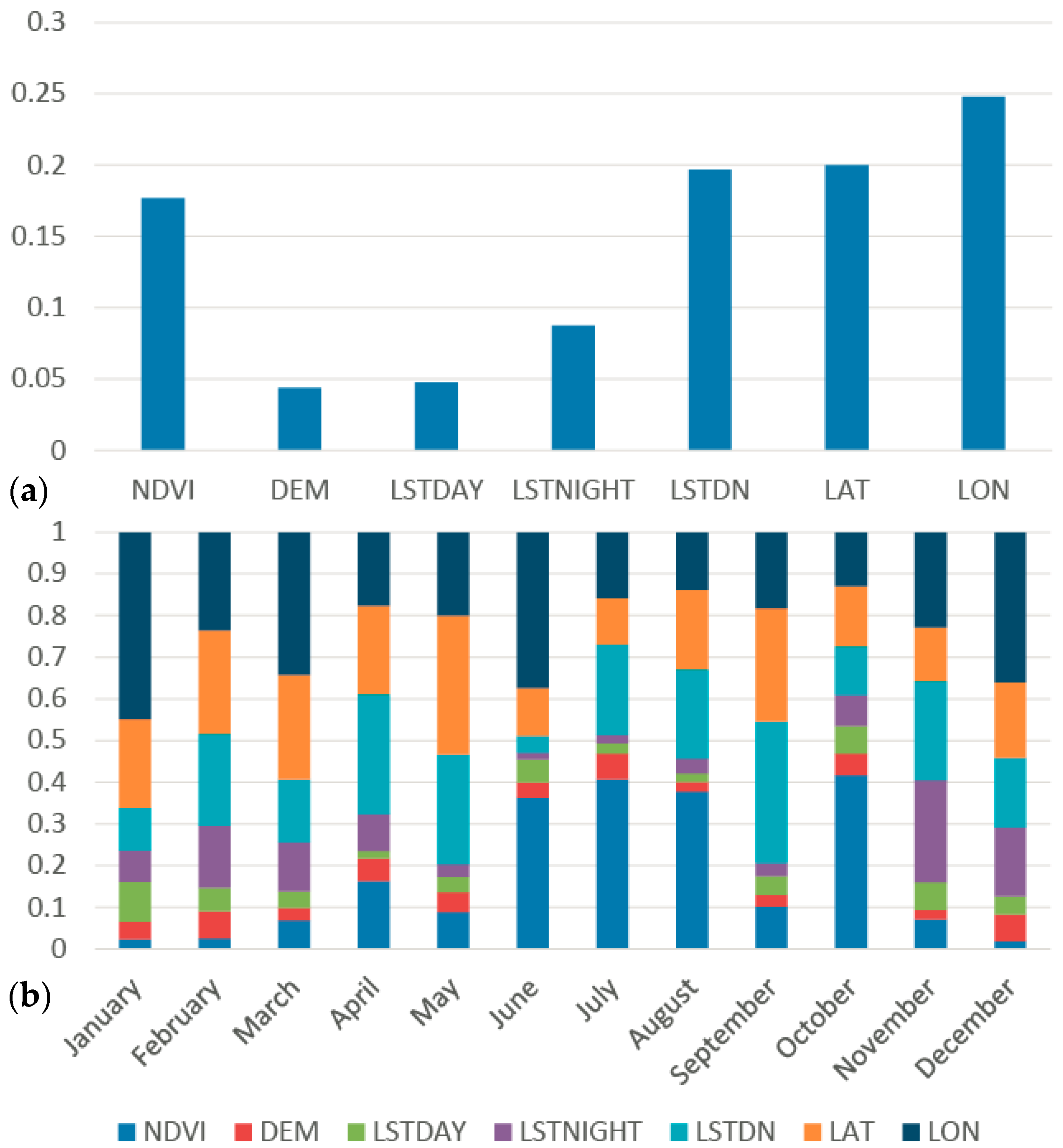
4.4. Variable Importance of Random Forests

The RF algorithm provides measurements of variable importance and these variable importance values are used to rank independent variables in terms of their contribution to the regression model. Figure 8a shows the average variable importance of each variable (VINDVI, VIDEM, VILSTDAY, VILSTNIGHT, VILSTDN, VILAT, and VILON). Figure 8b shows the average importance of each variable for each month from January to December. On average, VILON showed the highest importance, followed by VILAT, VILSTDN, VINDVI, VILSTNIGHT, VILSTDAY, and VIDEM, which indicates that the latitude and longitude were significant when downscaling the TRMM 3B43 V7 precipitation data over North China. This result occurred because precipitation varies spatially from east to west and north to south over the North China area. The day–night land surface temperature difference ranked just after latitude and longitude, highlighting the contribution of the land surface temperature feature to the downscaling model. As shown in Figure 8b, the variable importance values vary from January to December. This indicates that the significance of each variable for downscaling TRMM precipitation data over northern China can be very different in different months.

5. Discussion

The capability of NDVI and DEM for downscaling TRMM precipitation datasets has been investigated widely. First, the responses of vegetation to precipitation were acknowledged [55,56,57,58,59,60], and it was also found that vegetation can directly affect the humidity of the lower atmosphere by exerting a strong influence on the fluxes of sensible and latent heat into the atmosphere, thereby further influencing the development of moist convection both locally and at atmospheric circulation scales of tens to thousands of kilometers [61,62]. Second, topography can influence the regional atmospheric circulation and the spatial pattern of precipitation through its thermal and dynamic forcing mechanisms [63,64]. In theory, an increase of elevation could increase the relative humidity of air masses by expansion and cooling as the air masses rise, resulting in the occurrence of precipitation [65]. Additionally, the precipitation–NDVI relationship is susceptible to some human and natural factors that can limit the use of NDVI for downscaling satellite-based precipitation datasets over some regions [23]. The topography–precipitation relationship is also largely dependent on the fluctuations of the terrain: precipitation tends to not be affected by topography over regions where the topography is flat.
In this paper, we introduced land surface temperature as various factors for downscaling TRMM 3B43 data. The co-variability of surface temperature and precipitation has been observed globally [28]. As pointed out by Lemone et al. [66] and Trenberth et al. [28], if the ground is wet, more energy is likely to go into evaporation at the expense of sensible heating, so moisture acts as an “air conditioner”; and if the ground is wet from precipitation, then it is likely that associated clouds block the sun, resulting in less energy being provided in the first place and further reduction of temperature. Moreover, high rates of evaporation could occur directly from bare soil after periods of rain, further suppressing sensible heat and surface temperature [29,67]; thus, the surface temperature–precipitation relationship is more robust than the NDVI–precipitation relationship and the topography–precipitation relationship over regions of sparse vegetation such as barren lands and deserts. In this study, the land surface temperatures of both daytime and nighttime were included for the downscaling of TRMM 3B43 V7 precipitation datasets. It can be inferred from Figure 8 that the variable importance values of the day–night land surface temperature difference ranked higher than that of NDVI, indicating that the relationship between precipitation and land surface temperature is remarkable. However, the variable importance values of the different variables for downscaling TRMM precipitation data over northern China can be very different in different months. However, only three years of data were used in this study, and the variable importance values could be sensitive to single extreme precipitation events. The analysis of the importance of different variables is preliminary and the relationships between precipitation and these explanatory variables are very complex; further research is required to improve the downscaling algorithm.
Among the regression algorithms that were implemented in this study, RF produced the downscaled results with the highest accuracy both before and after residual correction, and MLR produced the results with the worst accuracy. For the other three algorithms, when residual correction was not implemented, CART ranked second after RF, followed by k-NN and SVM. The downscaled results of SVM after residual correction were improved significantly and produced an accuracy very similar to that of RF. There is one issue in this study that needs to be noted: we used a simple spline tension interpolator to interpolate the residual at coarse resolution to 1 km resolution. According to the results of previous downscaling algorithm studies, the residual of the models represents the precipitation that cannot be estimated by the models, and the spline tension interpolator [68] has been used widely in previous downscaling models to acquire interpolated residuals [6,22,23,25]. Additionally, the residual correction significantly improved the accuracy of the downscaled results by SVM. However, the SVM-based model performed poorly compared to CART, k-NN, and RF without residual correction. This indicates that the performance of SVM depended largely on the residual correction. Nevertheless, uncertainties could arise from the residual correction. First, the residuals were interpolated in only two dimensions, without consideration to the errors resulting from topography. Incorporating the impact of topography may be beneficial for improving the accuracy of the residual correction. Second, although the spline interpolation method is typically used for regularly spaced data, other interpolation algorithms (e.g., Kriging) need to be further examined experimentally to investigate the performance of different interpolation algorithms.

6. Conclusions

In this study, we introduced land surface temperature features in addition to NDVI, DEM, and geolocations for downscaling of monthly TRMM 3B43 V7 precipitation data from a spatial resolution of 0.25° to one of 1 km over North China. Four machine learning regression algorithms, CART, k-NN, SVM, and RF, were implemented for the purpose of comparison, and the downscaled results were validated based on observations from meteorological stations and also compared with the results of the multiple linear regression algorithm.
The validation results showed that the four machine learning algorithms outperformed the multiple linear regression algorithm and that the SVM and RF-based models produced the results with the highest accuracies, followed by CART and k-NN. However, the accuracy of downscaled results using SVM was largely dependent on residual correction. For each individual month, the downscaled results were well correlated with the observations, but the accuracies were relatively lower during July to September. Investigation of the relationship between the estimation errors and the precipitation observations showed that downscaling errors increase as monthly total precipitation increases, but the RF model was less affected by the proportional effect between errors and observations.
Moreover, the average variable importance values of geolocations (longitude and latitude) were higher than those of the other variables. Because the precipitation over North China is spatially heterogeneous [69], the inclusion of geolocations can be beneficial to the performance of the downscaling model. In addition, the variable importance values of the day–night land surface temperature difference were higher than those of NDVI. This highlights the significance of the precipitation–land surface temperature relationship when downscaling TRMM 3B43 V7 precipitation data.
In the future, the coupled relationships of precipitation with land surface temperature, vegetation, and topography should receive additional research to improve the accuracy of downscaling satellite-based precipitation datasets. Furthermore, weather radars offer an enormous potential to improve the accuracy of satellite-based precipitation datasets and can be also indicate not only where rainfall fell, but where the precipitation was transported to within the ephemeral stream network. Therefore, weather radars may be a useful substitute for downscaling TRMM 3B43 V7 precipitation data where the high-quality radar datasets are available. In addition, other land surface features related to precipitation (such as soil moisture, slope, and aspect) could be introduced to investigate whether these features are beneficial for downscaling satellite precipitation datasets. In addition, the relationship between precipitation and land surface temperature is more instant, making it more valuable to the downscaling of weekly or daily precipitation datasets, which has great significance for hydrological, meteorological, and ecological research.

Acknowledgments

This research was supported by the Geographic Resources and Ecology Knowledge Service System of China Knowledge Center for Engineering Sciences and Technology (No. CKCEST-2015-1-4), the National Special Program on Basic Science and Technology Research of China (No. 2013FY110900) and the National Data Sharing Infrastructure of Earth System Science. The authors are indebted to the National Aeronautics and Space Administration for providing the MODIS, TRMM, and DEM data that were used in this study. We also thank the National Data Sharing Infrastructure of Earth System Science for providing the boundary data of China. In addition, we would like to thank the anonymous reviewers for their helpful comments and suggestions in enhancing this manuscript.

Author Contributions

Wenlong Jing drafted the manuscript and was responsible for the research design, experiment, and analysis. Yaping Yang reviewed the manuscript and was responsible for the research design and analysis. Xiafang Yue and Xiaodan Zhao supported the data preparation and the interpretation of the results. All of the authors contributed to editing and reviewing the manuscript.

Conflicts of Interest

The authors declare no conflict of interest.

References

  1. Xie, P.; Xiong, A.-Y. A conceptual model for constructing high-resolution gauge-satellite merged precipitation analyses. J. Geophys. Res. 2011, 116. [Google Scholar] [CrossRef]
  2. Morrissey, M.L.; Maliekal, J.A.; Greene, J.S.; Wang, J. The uncertainty of simple spatial averages using rain gauge networks. Water Resour. Res. 1995, 31, 2011–2017. [Google Scholar] [CrossRef]
  3. Villarini, G.; Krajewski, W.F. Empirically-based modeling of spatial sampling uncertainties associated with rainfall measurements by rain gauges. Adv. Water Resour. 2008, 31, 1015–1023. [Google Scholar] [CrossRef]
  4. Krajewski, W.F.; Smith, J.A. Radar hydrology: rainfall estimation. Adv. Water Resour. 2002, 25, 1387–1394. [Google Scholar] [CrossRef]
  5. Mandapaka, P.V.; Krajewski, W.F.; Ciach, G.J.; Villarini, G.; Smith, J.A. Estimation of radar-rainfall error spatial correlation. Adv. Water Resour. 2009, 32, 1020–1030. [Google Scholar] [CrossRef]
  6. Immerzeel, W.W.; Rutten, M.M.; Droogers, P. Spatial downscaling of TRMM precipitation using vegetative response on the Iberian Peninsula. Remote Sens. Environ. 2009, 113, 362–370. [Google Scholar] [CrossRef]
  7. AghaKouchak, A.; Mehran, A.; Norouzi, H.; Behrangi, A. Systematic and random error components in satellite precipitation data sets. Geophys. Res. Lett. 2012, 39, 1–4. [Google Scholar] [CrossRef]
  8. Hsu, K.-l.; Gao, X.; Sorooshian, S.; Gupta, H.V. Precipitation estimation from remotely sensed information using artificial neural networks. J. Appl. Meteorol. 1997, 36, 1176–1190. [Google Scholar] [CrossRef]
  9. Huffman, G.J.; Adler, R.F.; Arkin, P.; Chang, A.; Ferraro, R.; Gruber, A.; Janowiak, J.; McNab, A.; Rudolf, B.; Schneider, U. The Global Precipitation Climatology Project (GPCP) combined precipitation dataset. Bull. Am. Meteorol. Soc. 1997, 78, 5–20. [Google Scholar] [CrossRef]
  10. Huffman, G.J.; Bolvin, D.T.; Nelkin, E.J.; Wolff, D.B.; Adler, R.F.; Gu, G.; Hong, Y.; Bowman, K.P.; Stocker, E.F. The TRMM Multisatellite Precipitation Analysis (TMPA): Quasi-global, multiyear, combined-sensor precipitation estimates at fine scales. J. Hydrometeorol. 2007, 8, 38–55. [Google Scholar] [CrossRef]
  11. Ricciardelli, E.; Cimini, D.; Di Paola, F.; Romano, F.; Viggiano, M. A statistical approach for rain intensity differentiation using Meteosat Second Generation–Spinning Enhanced Visible and InfraRed Imager observations. Hydrol. Earth Syst. Sci. 2014, 18, 2559–2576. [Google Scholar] [CrossRef] [Green Version]
  12. Casella, D.; Dietrich, S.; Di Paola, F.; Formenton, M.; Mugnai, A.; Porcù, F.; Sanò, P. PM-GCD—A combined IR–MW satellite technique for frequent retrieval of heavy precipitation. Nat. Hazards Earth Syst. Sci. 2012, 12, 231–240. [Google Scholar] [CrossRef]
  13. Di Paola, F.; Casella, D.; Dietrich, S.; Mugnai, A.; Ricciardelli, E.; Romano, F.; Sanò, P. Combined MW-IR Precipitation Evolving Technique (PET) of convective rain fields. Nat. Hazards Earth Syst. Sci. 2012, 12, 3557–3570. [Google Scholar] [CrossRef]
  14. Di Paola, F.; Ricciardelli, E.; Cimini, D.; Romano, F.; Viggiano, M.; Cuomo, V. Analysis of catania flash flood case study by using combined microwave and infrared technique. J. Hydrometeorol. 2014, 15, 1989–1998. [Google Scholar] [CrossRef]
  15. Munoz, E.A.; Di Paola, F.; Lanfri, M.; Arteaga, F.J. Observing the troposphere through the Advanced Technology Microwave Sensor (ATMS) to retrieve rain rate. IEEE Lat. Am. Trans. 2016, 14, 586–594. [Google Scholar] [CrossRef]
  16. Sanò, P.; Panegrossi, G.; Casella, D.; Di Paola, F.; Milani, L.; Mugnai, A.; Petracca, M.; Dietrich, S. The Passive microwave Neural network Precipitation Retrieval (PNPR) algorithm for AMSU/MHS observations: description and application to European case studies. Atmos. Meas. Tech. 2015, 8, 837–857. [Google Scholar] [CrossRef]
  17. Cimini, D.; Romano, F.; Ricciardelli, E.; Di Paola, F.; Viggiano, M.; Marzano, F.S.; Colaiuda, V.; Picciotti, E.; Vulpiani, G.; Cuomo, V. Validation of satellite OPEMW precipitation product with ground-based weather radar and rain gauge networks. Atmos. Meas. Tech. 2013, 6, 3181–3196. [Google Scholar] [CrossRef]
  18. Munoz, E.A.; Paola, F.D.; Lanfri, M. Advances on rain rate retrieval from satellite platforms using artificial neural networks. IEEE Lat. Am. Trans. 2015, 13, 3179–3186. [Google Scholar] [CrossRef]
  19. Kubota, T.; Shige, S.; Hashizume, H.; Aonashi, K.; Takahashi, N.; Seto, S.; Hirose, M.; Takayabu, Y.N.; Ushio, T.; Nakagawa, K.; et al. Global precipitation map using satellite-borne microwave radiometers by the GSMaP project: Production and validation. IEEE Trans. Geosci. Remote Sens. 2007, 45, 2259–2275. [Google Scholar] [CrossRef]
  20. Funk, C.; Peterson, P.; Landsfeld, M.; Pedreros, D.; Verdin, J.; Shukla, S.; Husak, G.; Rowland, J.; Harrison, L.; Hoell, A.; et al. The climate hazards infrared precipitation with stations—A new environmental record for monitoring extremes. Sci Data 2015, 2, 150066. [Google Scholar] [CrossRef] [PubMed]
  21. Funk, C.; Verdin, A.; Michaelsen, J.; Peterson, P.; Pedreros, D.; Husak, G. A global satellite-assisted precipitation climatology. Earth Syst. Sci. Data 2015, 7, 275–287. [Google Scholar] [CrossRef]
  22. Jia, S.; Zhu, W.; Lű, A.; Yan, T. A statistical spatial downscaling algorithm of TRMM precipitation based on NDVI and DEM in the Qaidam Basin of China. Remote Sens. Environ. 2011, 115, 3069–3079. [Google Scholar] [CrossRef]
  23. Xu, S.; Wu, C.; Wang, L.; Gonsamo, A.; Shen, Y.; Niu, Z. A new satellite-based monthly precipitation downscaling algorithm with non-stationary relationship between precipitation and land surface characteristics. Remote Sens. Environ. 2015, 162, 119–140. [Google Scholar] [CrossRef]
  24. Chen, C.; Zhao, S.; Duan, Z.; Qin, Z. An improved spatial downscaling procedure for TRMM 3B43 precipitation product using geographically weighted regression. IEEE J. Sel. Top. Appl. Earth Obs. Remote Sens. 2015, 8, 4592–4604. [Google Scholar] [CrossRef]
  25. Shi, Y.; Song, L.; Xia, Z.; Lin, Y.; Myneni, R.; Choi, S.; Wang, L.; Ni, X.; Lao, C.; Yang, F. Mapping annual precipitation across mainland China in the period 2001–2010 from TRMM3B43 product using spatial downscaling approach. Remote Sens. 2015, 7, 5849–5878. [Google Scholar] [CrossRef]
  26. Valentine, A.; Kalnins, L. An introduction to learning algorithms and potential applications in geomorphometry and earth surface dynamics. Earth Surf. Dyn. 2016, 4, 445–460. [Google Scholar] [CrossRef]
  27. Lary, D.J.; Alavi, A.H.; Gandomi, A.H.; Walker, A.L. Machine learning in geosciences and remote sensing. Geosci. Front. 2016, 7, 3–10. [Google Scholar] [CrossRef]
  28. Trenberth, K.E.; Shea, D.J. Relationships between precipitation and surface temperature. Geophys. Res. Lett. 2005, 32. [Google Scholar] [CrossRef]
  29. De Kauwe, M.G.; Taylor, C.M.; Harris, P.P.; Weedon, G.P.; Ellis, R.J. Quantifying land surface temperature variability for two sahelian mesoscale regions during the wet season. J. Hydrometeorol. 2013, 14, 1605–1619. [Google Scholar] [CrossRef]
  30. Xu, X.; Lu, C.; Shi, X.; Ding, Y. Large-scale topography of China: A factor for the seasonal progression of the Meiyu rainband? J. Geophys. Res. 2010, 115. [Google Scholar] [CrossRef]
  31. The National Meteorological Information Center. Available online: http://data.cma.cn/site/index.html (accessed on 11 October 2016).
  32. Yang, F.; Lau, K.M. Trend and variability of China precipitation in spring and summer: Linkage to sea-surface temperatures. Int. J. Climatol. 2004, 24, 1625–1644. [Google Scholar] [CrossRef]
  33. Zhai, P.; Zhang, X.; Wan, H.; Pan, X. Trends in total precipitation and frequency of daily precipitation extremes over China. J. Clim. 2005, 18, 1096–1108. [Google Scholar] [CrossRef]
  34. Ma, Z. Interannual characteristics of the surface hydrological variables over the arid and semi-arid areas of northern China. Glob. Planet. Chang. 2003, 37, 189–200. [Google Scholar] [CrossRef]
  35. Li, B.; Tao, S.; Dawson, R.W. Relations between AVHRR NDVI and ecoclimatic parameters in China. Int. J.Remote Sens. 2002, 23, 989–999. [Google Scholar] [CrossRef]
  36. Jingyong, Z.; Wenjie, D.; Congbin, F.; Lingyun, W. The influence of vegetation cover on summer precipitation in China: A statistical analysis of NDVI and climate data. Adv. Atmos. Sci. 2003, 20, 1002–1006. [Google Scholar] [CrossRef]
  37. Wan, Z.; Wang, P.; Li, X. Using MODIS land surface temperature and Normalized Difference Vegetation Index products for monitoring drought in the southern Great Plains, USA. Int. J. Remote Sens. 2004, 25, 61–72. [Google Scholar] [CrossRef]
  38. The National Aeronautics and Space Administration (NASA) Precipitation Measurement Missions (PMM). Available online: http://pmm.nasa.gov/TRMM/trmm-instruments (accessed on 11 October 2016).
  39. The NASA Land Processes Distributed Active Archive Center (LP DAAC). Available online: https://lpdaac.usgs.gov/ (accessed on 11 October 2016).
  40. Jarvis, A.; Reuter, H.I.; Nelson, A.; Guevara, E. Hole-Filled SRTM for the Globe Version 4, Available from the CGIAR-CSI SRTM 90m Database. Available online: http://srtm.csi.cgiar.org/ (accessed on 31 January 2016).
  41. Rokach, L.; Maimon, O. Data Mining with Decision Trees: Theory and Applications; World Scientific Pub Co. Inc.: Singapore, 2008. [Google Scholar]
  42. Breiman, L.; Friedman, J.H.; Olshen, R.A.; Stone, C.J. Classification and Regression Trees; Chapman and Hall/CRC: Boca Raton, FL, USA, 1984. [Google Scholar]
  43. Altman, N.S. An introduction to kernel and nearest-neighbor nonparametric regression. Am. Stat. 1992, 46, 175–185. [Google Scholar]
  44. Ahmad, S.; Kalra, A.; Stephen, H. Estimating soil moisture using remote sensing data: A machine learning approach. Adv. Water Resour. 2010, 33, 69–80. [Google Scholar] [CrossRef]
  45. Weng, Q. Remote sensing of impervious surfaces in the urban areas: Requirements, methods, and trends. Remote Sens. Environ. 2012, 117, 34–49. [Google Scholar] [CrossRef]
  46. Mountrakis, G.; Im, J.; Ogole, C. Support vector machines in remote sensing: A review. ISPRS J. Photogramm. Remote Sens. 2011, 66, 247–259. [Google Scholar] [CrossRef]
  47. Vapnik, V. The Nature of Statistical Learning Theory; Springer: New York, NY, USA, 1995. [Google Scholar]
  48. Vapnik, V. Statistical Learning Theory; Wiley: New York, NY, USA, 1998. [Google Scholar]
  49. Gislason, P.O.; Benediktsson, J.A.; Sveinsson, J.R. Random Forests for land cover classification. Pattern Recognit. Lett. 2006, 27, 294–300. [Google Scholar] [CrossRef]
  50. Breiman, L. Random Forests. Mach. Learn. 2001, 45, 5–32. [Google Scholar] [CrossRef]
  51. Pedregosa, F.; Varoquaux, G.; Gramfort, A.; Michel, V.; Thirion, B.; Grisel, O.; Blondel, M.; Prettenhofer, P.; Weiss, R.; Dubourg, V.; et al. Scikit-learn: Machine Learning in Python. J. Mach. Learn. Res. 2011, 12, 2825–2830. [Google Scholar]
  52. Li, C.; Wang, J.; Wang, L.; Hu, L.; Gong, P. Comparison of Classification Algorithms and Training Sample Sizes in Urban Land Classification with Landsat Thematic Mapper Imagery. Remote Sens. 2014, 6, 964–983. [Google Scholar] [CrossRef]
  53. Harrington, P. Machine Learning in Action; Manning Publications: Greenwich, CT, USA, 2012. [Google Scholar]
  54. Hand, D.J.; Mannila, H.; Smyth, P. Principles of Data Mining; The MIT Press: Cambridge, MA, USA; London, UK, 2001; p. 546. [Google Scholar]
  55. Zhang, X.; Friedl, M.A.; Schaaf, C.B.; Strahler, A.H.; Liu, Z. Monitoring the response of vegetation phenology to precipitation in Africa by coupling MODIS and TRMM instruments. J. Geophys. Res. Atmos. 2005, 110. [Google Scholar] [CrossRef]
  56. Wang, J.; Price, K.P.; Rich, P.M. Spatial patterns of NDVI in response to precipitation and temperature in the central Great Plains. Int. J. Remote Sens. 2001, 22, 3827–3844. [Google Scholar] [CrossRef]
  57. Vicente-Serrano, S.M.; Gouveia, C.; Camarero, J.J.; Beguería, S.; Trigo, R.; López-Moreno, J.I.; Azorín-Molina, C.; Pasho, E.; Lorenzo-Lacruz, J.; Revuelto, J.; et al. Response of vegetation to drought time-scales across global land biomes. Proc. Natl. Acad. Sci. USA 2013, 110, 52–57. [Google Scholar] [CrossRef] [PubMed] [Green Version]
  58. Zhong, L.; Ma, Y.; Salama, M.S.; Su, Z. Assessment of vegetation dynamics and their response to variations in precipitation and temperature in the Tibetan Plateau. Clim. Chang. 2010, 103, 519–535. [Google Scholar] [CrossRef]
  59. Barbosa, H.A.; Huete, A.R.; Baethgen, W.E. A 20-year study of NDVI variability over the Northeast Region of Brazil. J. Arid Environ. 2006, 67, 288–307. [Google Scholar] [CrossRef]
  60. Barbosa, H.A.; Lakshmi Kumar, T.V. Influence of rainfall variability on the vegetation dynamics over Northeastern Brazil. J. Arid Environ. 2016, 124, 377–387. [Google Scholar] [CrossRef]
  61. Taylor, C.M.; de Jeu, R.A.M.; Guichard, F.; Harris, P.P.; Dorigo, W.A. Afternoon rain more likely over drier soils. Nature 2012, 489, 423–426. [Google Scholar] [CrossRef] [PubMed] [Green Version]
  62. Spracklen, D.V.; Arnold, S.R.; Taylor, C.M. Observations of increased tropical rainfall preceded by air passage over forests. Nature 2012, 489, 282–285. [Google Scholar] [CrossRef] [PubMed]
  63. Guan, H.; Wilson, J.L.; Xie, H. A cluster-optimizing regression-based approach for precipitation spatial downscaling in mountainous terrain. J. Hydrol. 2009, 375, 578–588. [Google Scholar] [CrossRef]
  64. Yin, Z.Y.; Zhang, X.; Liu, X.; Colella, M.; Chen, X. An assessment of the biases of satellite rainfall estimates over the Tibetan Plateau and correction methods based on topographic analysis. J. Hydrometeorol. 2008, 9, 301–326. [Google Scholar] [CrossRef]
  65. Sokol, Z.; Bližňák, V. Areal distribution and precipitation-altitude relationship of heavy short-term precipitation in the Czech Republic in the warm part of the year. Atmos. Res. 2009, 94, 652–662. [Google Scholar] [CrossRef]
  66. Lemone, M.A.; Grossman, R.L.; Chen, F.; Ikeda, K.; Yates, D. Choosing the Averaging interval for comparison of observed and modeled fluxes along aircraft transects over a heterogeneous surface. J. Hydrometeorol. 2003, 4, 179–195. [Google Scholar] [CrossRef]
  67. Wallace, J.S.; Holwill, C.J. Soil evaporation from tiger-bush in south-west Niger. J. Hydrol. 1997, 188, 426–442. [Google Scholar] [CrossRef]
  68. Franke, R. Smooth interpolation of scattered data by local thin plate splines. Comput. Math. Appl. 1982, 8, 273–281. [Google Scholar] [CrossRef]
  69. Chen, F.; Liu, Y.; Liu, Q.; Li, X. Spatial downscaling of TRMM 3B43 precipitation considering spatial heterogeneity. Int. J. Remote Sens. 2014, 35, 3074–3093. [Google Scholar] [CrossRef]
Figure 1. Elevation and distribution of meteorological stations in North China.
Remotesensing 08 00835 g001
Figure 2. Average monthly total precipitation and monthly average temperature of the North China area.
Remotesensing 08 00835 g002
Figure 3. Flowchart of the downscaling algorithm used in this study.
Remotesensing 08 00835 g003
Figure 4. (a) TRMM 3B43 V7 precipitation data and downscaled results before residual correction of (b) MLR; (c) CART; (d) k-NN; (e) SVM; and (f) RF in May 2006.
Remotesensing 08 00835 g004
Figure 5. Interpolated residuals of downscaling models in May 2006: (a) MLR; (b) CART; (c) k-NN; (d) SVM; (e) RF.
Remotesensing 08 00835 g005
Figure 6. (a) TRMM 3B43 V7 precipitation data and downscaled results after residual correction of (b) MLR; (c) CART; (d) k-NN; (e) SVM; and (f) RF in May 2006.
Remotesensing 08 00835 g006
Figure 7. Scatter plots between averaged MAE of downscaled results for each station and average precipitation observations of the stations: (a) CART; (b) k-NN; (c) SVM; and (d) RF.
Remotesensing 08 00835 g007
Figure 8. (a) Average importance of each variable; (b) average importance of each variable in each month.
Remotesensing 08 00835 g008
Table 1. Parameter combinations for each algorithm.
AlgorithmAbbreviationParameter TypeParameters
Classification and Regression TreeCARTMinSamplesLeaf1, 2, 3, 4, 5, 6, 7, 8, 9, 10
k-Nearest Neighborsk-NNn_neighbors3, 5, 7, 9, 11, 13, 15, 17, 19
Support Vector MachineSVMKernelrbf
Cost(C)20, 40, 60, 80, 100, 150, 200, 220, 250, 280, 300
gamma2−4, 2−3, 2−2, 2−1, 1, 21, 22, 23, 24
Random ForestsRFn_estimators20, 40, 60, 80, 100, 120, 140, 160, 180, 200
MinSamplesLeaf: The minimum number of samples required to be at a leaf node; n_neighbors: Number of neighbors to use; Kernel: Specifies the kernel type to be used in the algorithm; rbf: Radial basis function; Cost(C): Penalty parameter C of the error term; gamma: Kernel coefficient for ‘rbf’.
Table 2. The coefficients of determination (R2), mean absolute error (MAE), and root mean square error (RMSE) of the simulated values using the different algorithms compared to the original TRMM 3B43 V7 data.
MonthMLRCARTk-NNSVMRF
R2MAERMSER2MAERMSER2MAERMSER2MAERMSER2MAERMSE
(mm)(mm)(mm)(mm)(mm)(mm)(mm)(mm)(mm)(mm)
January0.2694.27.00.9230.92.30.7971.73.70.6861.94.30.9850.41.0
February0.4294.87.40.9830.51.00.8352.14.00.7842.04.10.9890.51.0
March0.4575.28.20.9431.12.40.8382.44.50.7043.16.10.9850.71.3
April0.53210.716.00.9582.14.50.8634.68.70.8853.68.00.9861.32.7
May0.57713.518.60.9174.37.50.8446.410.50.7717.412.70.9831.93.4
June0.66321.930.80.9516.111.10.8889.816.40.65317.728.80.9892.95.1
July0.69526.638.30.968.714.10.92212.719.40.70924.737.70.9924.06.2
August0.6924.735.50.9795.59.60.9439.415.10.85814.925.00.9943.05.0
September0.5817.024.10.9624.78.10.9336.610.80.8410.116.70.9922.13.6
October0.57710.715.70.9812.34.30.8954.98.60.856.511.80.9911.32.4
November0.5286.910.40.9561.63.10.8982.64.80.8413.05.70.9920.71.3
December0.3493.96.00.9190.71.50.8431.12.20.7181.52.90.9870.30.6
Average0.52912.518.20.9532.95.30.7971.73.70.7747.312.50.9891.52.6
Table 3. Validation results of each algorithm before residual correction.
MonthMLRCARTk-NNSVMRF
R2MAERMSER2MAERMSER2MAERMSER2MAERMSER2MAERMSE
(mm)(mm)(mm)(mm)(mm)(mm)(mm)(mm)(mm)(mm)
January0.0344.813.00.6373.05.10.5763.25.00.5433.04.90.6313.15.4
February0.0398.223.10.7214.36.70.7154.26.10.6374.46.70.774.16.0
March0.077.317.50.6684.66.60.6444.76.40.4344.88.50.6964.66.5
April0.07118.656.10.69410.215.80.699.914.60.7149.013.90.7879.012.9
May0.2119.936.80.59712.918.20.6112.917.40.60512.717.60.6911.415.5
June0.12636.387.90.70221.931.90.70121.931.70.59325.137.00.78119.627.6
July0.28443.870.70.66830.742.80.62631.544.90.53837.050.20.72628.538.8
August0.22744.389.60.65628.040.90.64229.042.30.63229.343.70.72925.636.7
September0.21825.940.20.6815.922.50.64616.523.80.60318.025.10.75414.219.8
October0.20618.845.60.69910.316.40.73310.115.20.61411.418.00.7879.313.9
November0.07911.725.50.7356.59.50.7036.69.60.7166.38.90.7925.98.2
December0.0385.713.40.643.35.40.5813.35.10.5393.35.20.6763.35.1
Average0.13320.443.30.67712.618.50.65712.818.50.59713.720.00.73611.616.4
Table 4. Validation results of each algorithm after residual correction.
MonthMLRCARTk-NNSVMRF
R2MAERMSER2MAERMSER2MAERMSER2MAERMSER2MAERMSE
(mm)(mm)(mm)(mm)(mm)(mm)(mm)(mm)(mm)(mm)
January0.3553.58.30.6043.05.70.5593.25.90.5723.05.80.5932.95.8
February0.225.916.30.7044.16.70.7424.16.30.7214.06.40.744.06.3
March0.4585.29.50.6724.56.70.6654.56.50.6384.56.70.6844.46.6
April0.38211.828.40.7289.715.10.7758.913.10.7688.513.10.7948.512.4
May0.45316.833.70.63812.517.10.70811.215.00.72510.514.40.71210.914.8
June0.46325.748.90.73820.729.90.76520.028.40.79518.826.40.79718.626.3
July0.53832.852.10.72328.539.20.7128.340.20.77726.134.70.7626.236.1
August0.55230.752.20.69326.438.70.726.538.70.74524.536.00.75524.134.9
September0.57716.627.40.72414.721.00.72514.421.10.77813.719.10.77713.118.7
October0.61711.423.40.7399.915.20.7998.913.40.8028.412.60.8088.813.1
November0.5417.513.10.746.39.60.7376.29.40.7655.98.70.7815.78.5
December0.3143.98.40.6743.25.30.6453.25.20.6343.15.20.6923.15.1
Average0.45614.326.80.69811.917.50.71111.617.00.72710.915.80.74210.915.7

