
A New Image Processing Procedure Integrating PCI-RPC and ArcGIS-Spline Tools to Improve the Orthorectification Accuracy of High-Resolution Satellite Imagery


Abstract
:
1. Introduction
2. Methodology
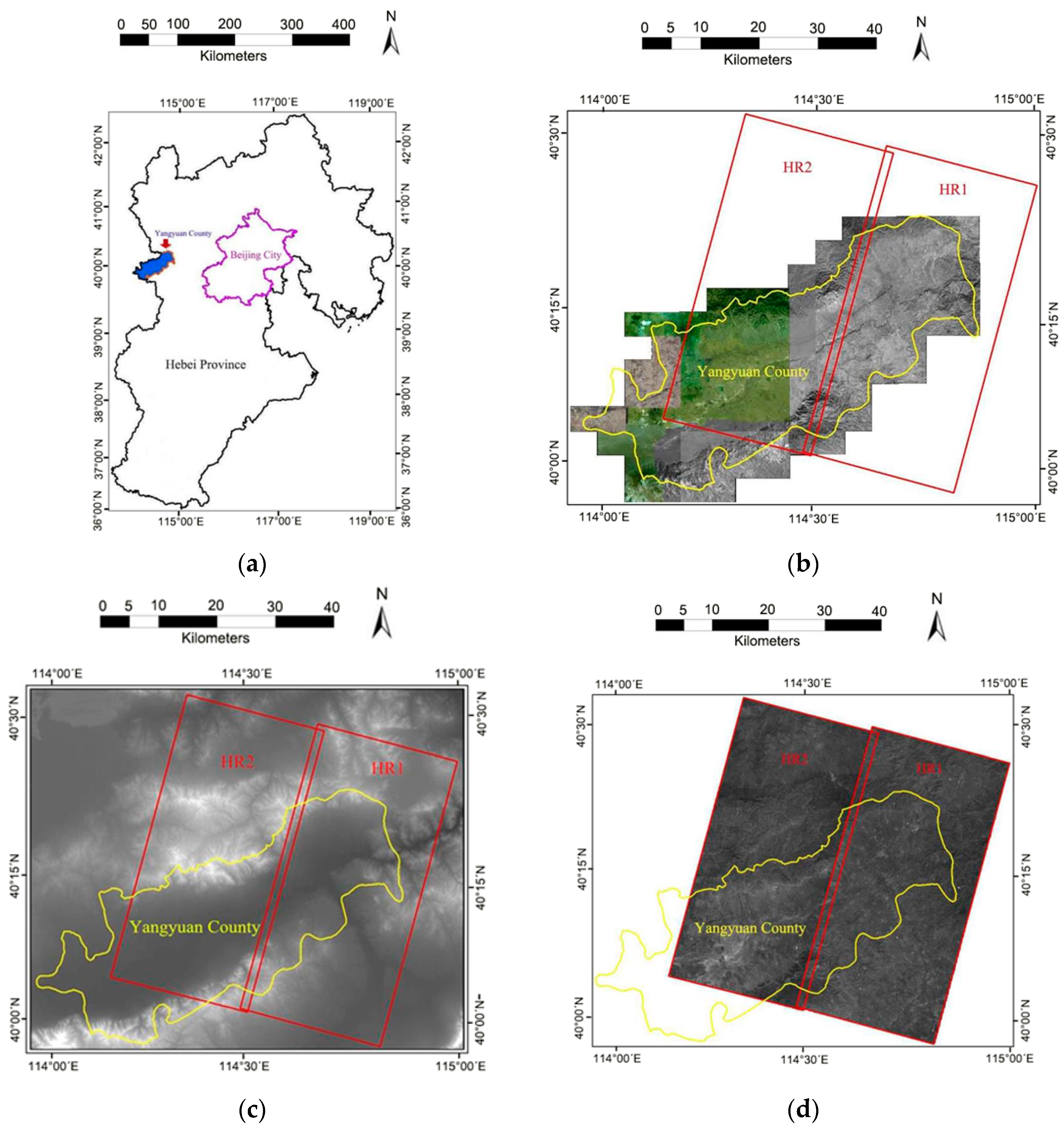
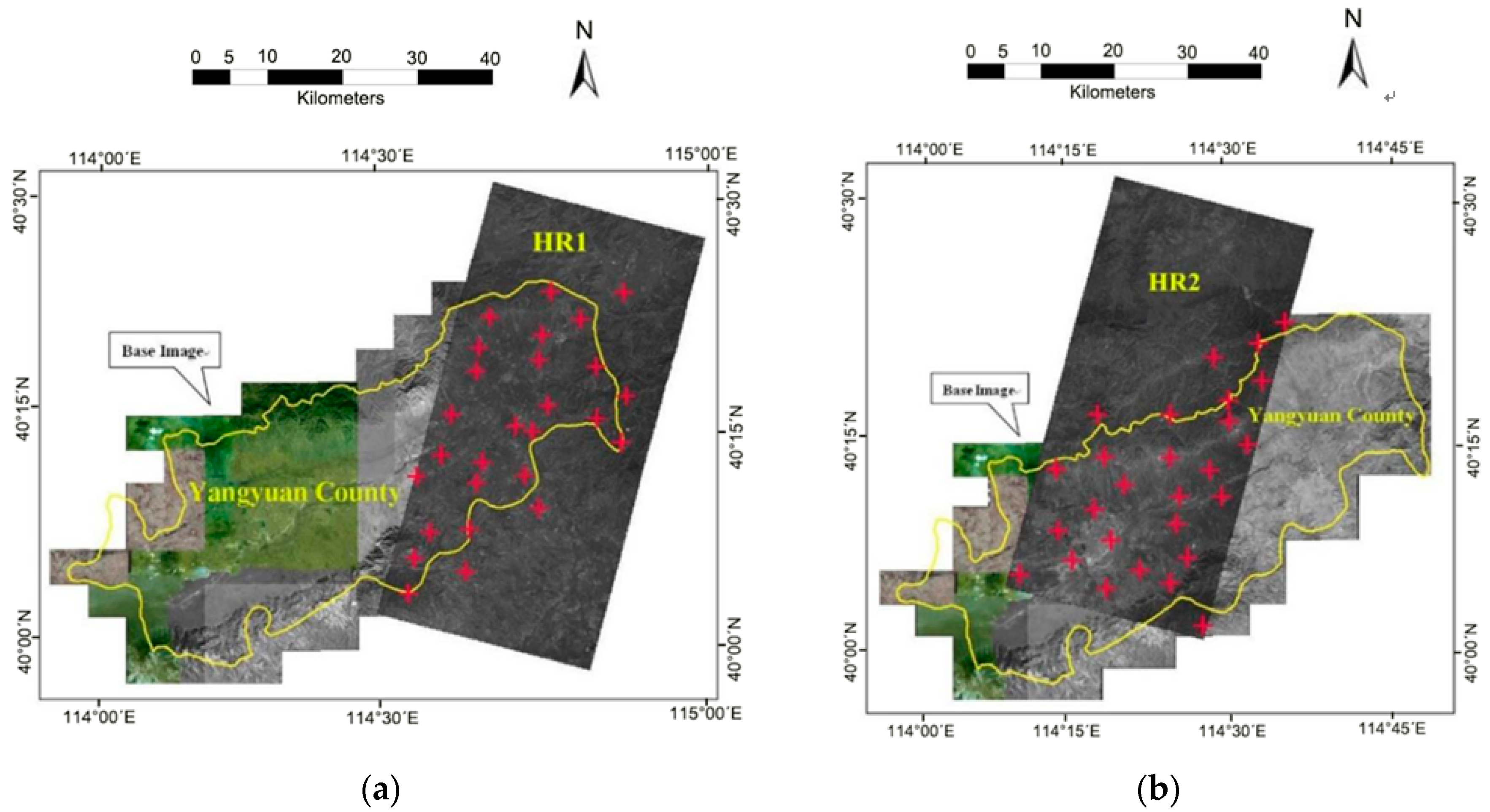
2.1. Study Area
2.2. Data Sets
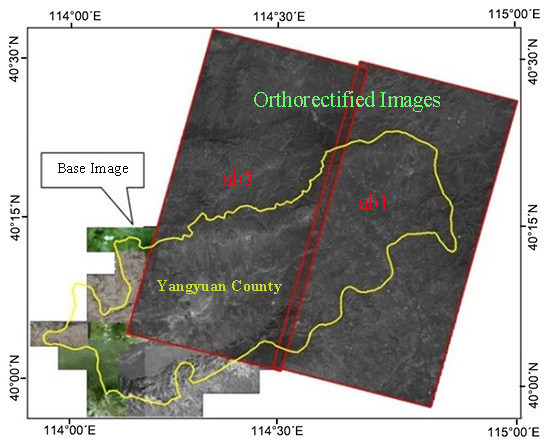
- Base image: An image of the second national land survey of China was collected to be used as a base image (Ministry of Land and Resources of People’s Republic of China), which was shown in Figure 1b.
- Warp images: High resolution CBERS-02C HR satellite images, track number No. ZY02C-HRC-E114.6_N40.3_20140904 _L1C0001836234, including two scenes, HR1 and HR2, with GeoTiff format were acquired from Yangyuan County, Hebei Province, China, on 4 September 2014, which was shown in Figure 1d. Both HR1 and HR2 scenes covered most of mountainous areas with a greater topographic relief. As China’s first satellite of land and resources, CBERS-02C carries a P/MS multi-spectral camera and two high resolution cameras (HRCs). The P/MS cameras can provide multispectral data with 10 m spatial resolution (MUS image) covering visible and near-infrared spectral regions with three bands: band2 (0.52–0.59 μm), band3 (0.63–0.69 μm), and band4 (0.77–0.89 μm), and one panchromatic band image (PAN image) with 5 m spatial resolution covering spectral range 0.51–0.85 μm (band1). The HRC cameras can acquire 2.36 m spatial resolution image, covering spectral range 0.50–0.80 μm [26]. In this study, only two scenes of HRC images (HR1 and HR2) were tested.
2.3. Rectification Models
2.3.1. Polynomial Rectification Model
2.3.2. RPC Rectification Model
2.3.3. Spline Function Model
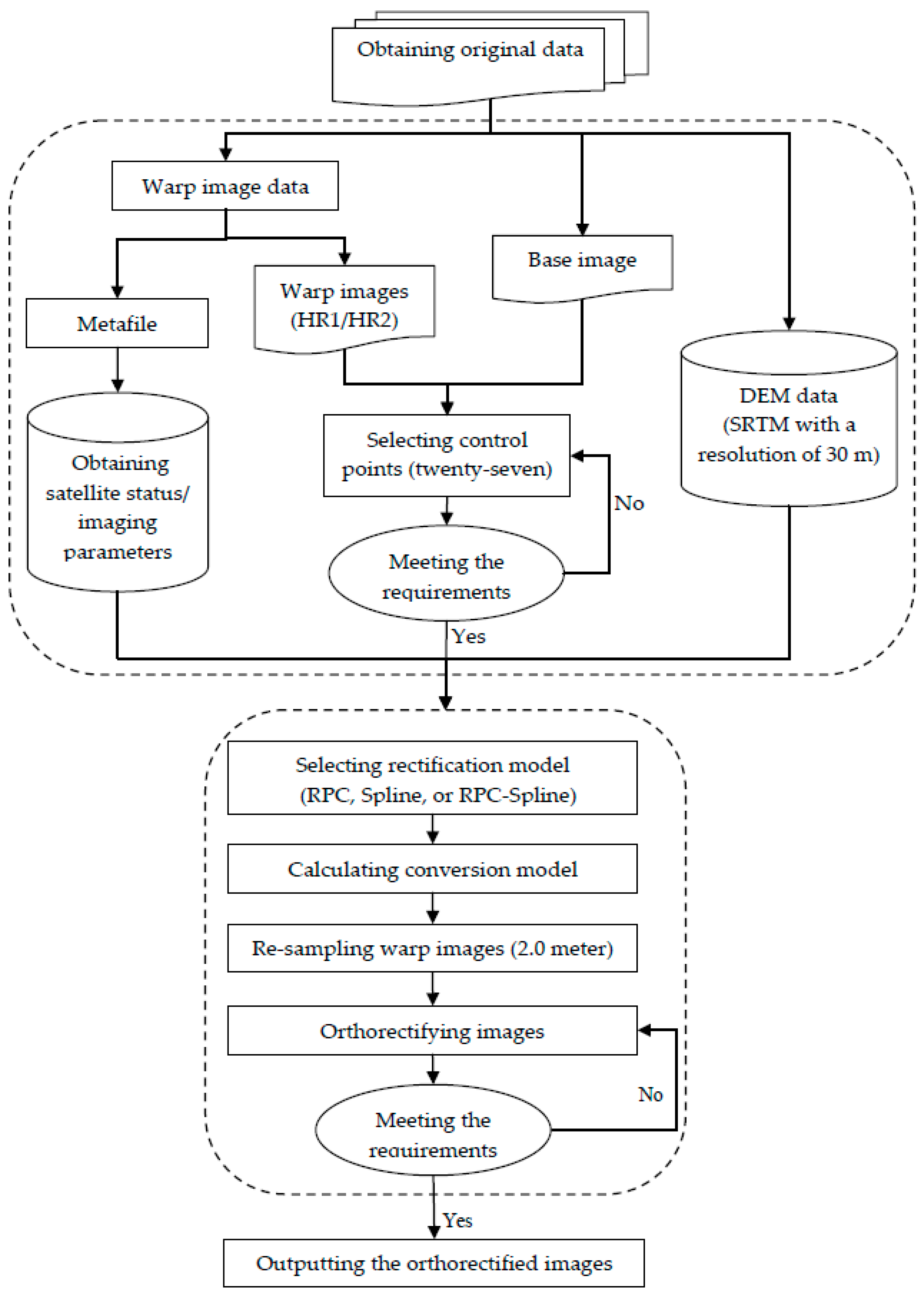
2.4. A Procedureof Orthorectification
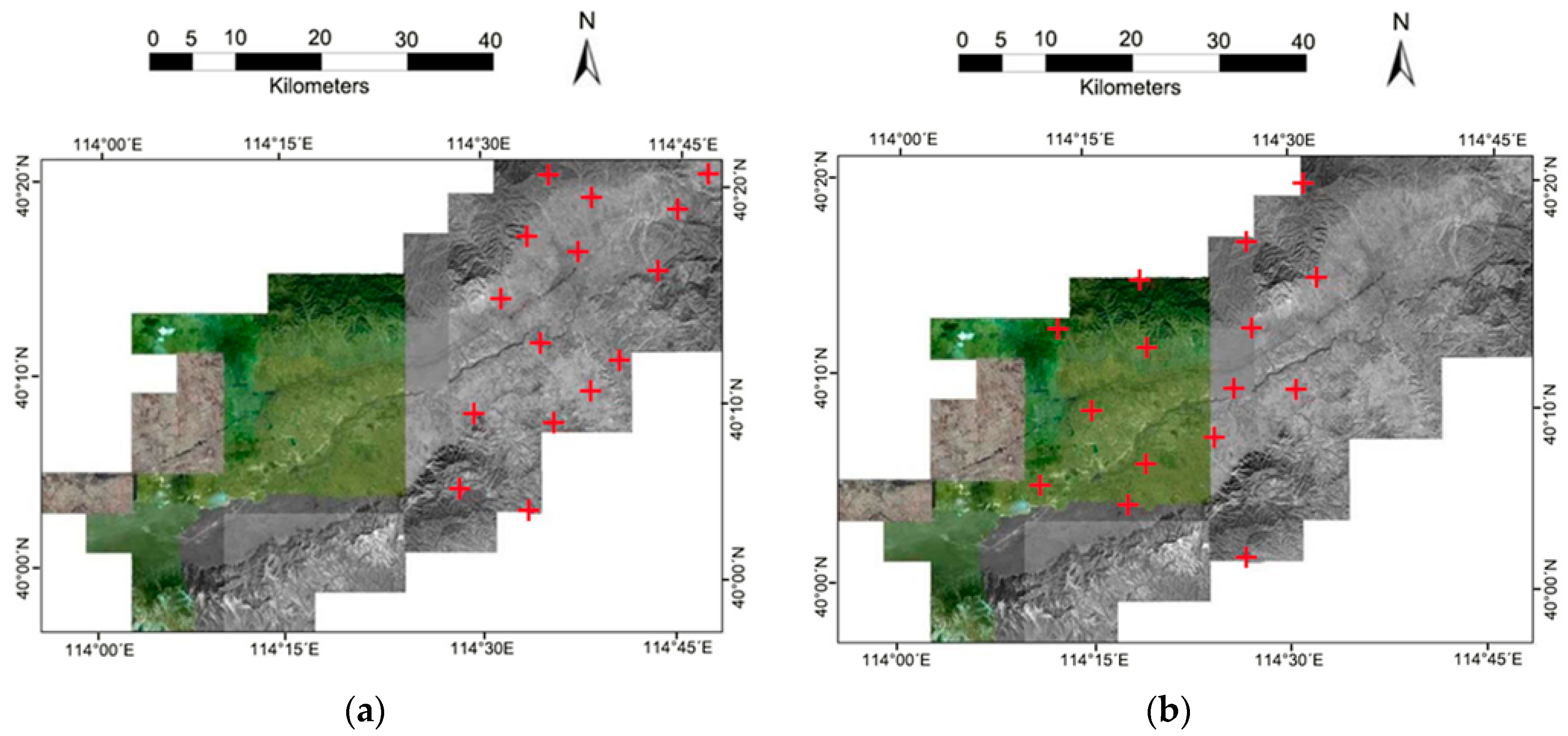
- The mean residual errors (i.e., RMSEs) of GCPs should be controlled in one pixel in the plains and hills, two pixels in the mountains. In this study, because the re-sampling pixel size is 2.0 m and the study area was featured with mountainous areas mixed with a portion of plain area, the RMSEs of GCPs should be controlled from 2.0 m to 4.0 m [18,45].
3. Experiment and Results
3.1. Orthorectification by PCI-RPC Tool
3.2. Geometric Correction by the ArcGIS-Spline Tool
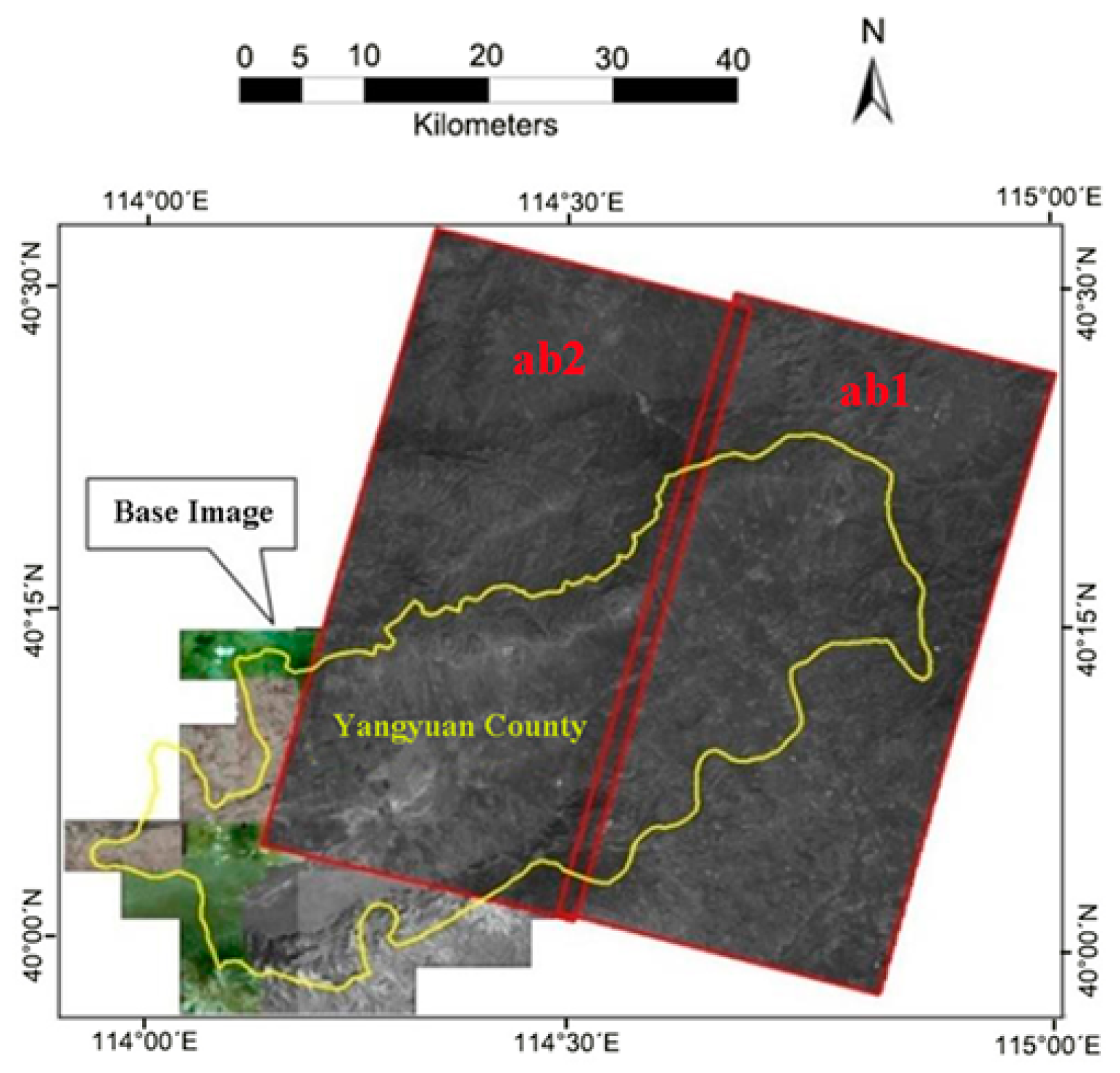
3.3. Integrating the PCI-RPC and ArcGIS-Spline Tools
3.4. Comparison of Image Rectification Approaches
- The accuracy of validation GCPs was consistently the highest for images ab1/ab2 among the three sets of geometrically corrected images, which indicates that the orthorectification accuracy has been significantly improved by using the new image processing procedure of integrating PCI software with the RPC orthorectification model and ArcGIS-Spline tool [49];
- The accuracy of validation GCPs was consistently the lowest for images b1/b2, which means that although running the ArcGIS-Spline tool could lead to high geometrical correction accuracy for the calibration GCPs in Table 2, for the other areas in the corrected images, the geometrical correction accuracy is actually very low, as the Spline model only works well for local geometric correction around GCPs without considering the topographic relief in the study area [20,42,43];
- The accuracy of validation GCPs was secondary for images a1/a2 among the three sets of corrected images, which means that when conducting image geometric correction, incorporating DEM data (thus called orthorectification) will help improve the image geometric correction accuracy compared with the case without using DEM data in image geometric rectification.
4. Discussion
5. Conclusions
Acknowledgments
Author Contributions
Conflicts of Interest
References
- Jaiswal, R.K.; Saxena, R.; Mukherjee, S. Application of remote sensing technology for land use/land cover change analysis. J. Indian Soc. Remote Sens. 1999, 27, 123–128. [Google Scholar] [CrossRef]
- Boccardo, P.; Mondino, E.B.; Tonolo, F.G.; Lingua, A. Orthorectification of high resolution satellite images. ISPRS Congr. 2004, 35, 1682–1750. [Google Scholar]
- Kali, E.S.; Leif, G.O.; Nathan, J.H.; Patrick, L.B.; Marvin, E.B. Extending satellite remote sensing to local scales: Land and water resource monitoring using high-resolution imagery. Remote Sens. Environ. 2003, 88, 144–156. [Google Scholar]
- Kasper, J.; Nicholas, C.C.; Sarah, E.G.; Yulia, S. Application of high spatial resolution satellite imagery for riparian and forest ecosystem classification. Remote Sens. Environ. 2007, 110, 29–44. [Google Scholar]
- Duccio, R. Effects of spatial and spectral resolution in estimating ecosystem α-diversity by satellite imagery. Remote Sens. Environ. 2007, 111, 423–434. [Google Scholar]
- Leprince, S.; Barbot, S.; Ayoub, F.; Avouac, J.P. Automatic and precise orthorectification, coregistration, and subpixel correlation of satellite images, application to ground deformation measurements. IEEE Trans. Geosci. Remote Sens. 2007, 45, 1529–1558. [Google Scholar] [CrossRef]
- Chmiel, J.; Kay, S.; Spruyt, P. Orthorectification and geometric quality assessment of very high spatial resolution satellite imagery for Common Agricultural Policy purposes. In Proceedings of the XXth ISPRS Congress, Istanbul, Turkey, 12–23 July 2004.
- Nichol, J.E.; Shaker, A.; Wong, M.-S. Application of high-resolution stereo satellite images to detailed landslide hazard assessment. Geomorphology 2006, 76, 68–75. [Google Scholar] [CrossRef]
- Dowman, I.; Dare, P. Automated procedures for multisensor registration and orthorectification of satellite images. Int. Arch. Photogramm. Remote Sens. 1999, 32, 4–3. [Google Scholar]
- Davis, C.H.; Wang, X. Urban land cover classification from high resolution multi-spectral Ikonos imagery. In Proceedings of the IEEE International Geoscience and Remote Sensing Symposium, Piscataway, NJ, USA, 24–28 June 2002.
- Marsetic, A.; Ostir, K.; Fras, M.K. Automatic orthorectification of high-resolution optical satellite images using vector roads. IEEE Trans. Geosci. Remote Sens. 2015, 53, 6035–6047. [Google Scholar] [CrossRef]
- Chen, L.-C.; Teo, T.-A.; Rau, J.-Y. Optimized patch back projection in orthorectification for high resolution satellite images. Int. Arch. Photogramm. Remote Sens. 2004, 35, 586–591. [Google Scholar]
- Fraser, C.S.; Dial, G.; Grodecki, J. Sensor orientation via RPCs. ISPRS J. Photogramm. Remote Sens. 2006, 60, 182–194. [Google Scholar] [CrossRef]
- Grodecki, J.; Dial, G. IKONOS geometric accuracy. In Proceedings of the Joint Workshop of ISPRS Working Groups I/2, I/5 and IV/7 on High Resolution Mapping from Space, Athens, GE, USA, 29–31 October 2001.
- Hu, Y.; Tao, C.V. Updating solutions of the rational function model using additional control information. Photogramm. Eng. Remote Sens. 2002, 68, 715–724. [Google Scholar]
- Je, C.; Park, H.-M. Homographic p-norms: Metrics of homographic image transformation. Signal Process. Image Commun. 2015, 39, 185–201. [Google Scholar] [CrossRef]
- DeTone, D.; Malisiewicz, T.; Rabinovich, A. Deep Image Homography Estimation. Available online: https://arxiv.org/abs/1606.03798 (accessed on 8 October 2016).
- Aguilar, M.A.; Aguera, F.; Aguilar, F.J.; Carvajal, F. Geometric accuracy assessment of the orthorectification process from very high resolution satellite imagery for Common Agricultural Policy purposes. Int. J. Remote Sens. 2008, 29, 7181–7197. [Google Scholar] [CrossRef]
- Topan, H.; Oruc, M.; Taskanat, T.; Cam, A. Combined efficiency of RPC and DEM accuracy on georeferencing accuracy of orthoimage: Case study with pleiades panchromatic mono image. IEEE Geosci. Remote Sens. 2014, 11, 1148–1152. [Google Scholar] [CrossRef]
- Tao, C.V.; Hu, Y. A comprehensive study of the rational function model for photogrammetric processing. Photogram. Eng. Remote Sens. 2001, 67, 1347–1357. [Google Scholar]
- Fabio, M.A.F.; Alexander, P.T.; Konstantin, V.K.; Yi, L.; Stefan, W. Impact of orthorectification and spatial sampling on maximum NDVI composite data in mountain regions. Remote Sens. Environ. 2009, 113, 2701–2712. [Google Scholar]
- Sowter, A. Orthorectification and interpretation of differential InSAR data over mountainous areas: A case study of the May 2008 Wenchuan Earthquake. Int. J. Remote Sens. 2010, 31, 3435–3448. [Google Scholar] [CrossRef]
- Childs, C. Interpolating surfaces in ArcGIS spatial analyst. ArcUser 2004, 32–35. [Google Scholar]
- Yang, J.S.; Wang, Y.Q.; August, P.V. Estimation of land surface temperature using spatial interpolation and satellite-derived surface emissivity. J. Environ. Inform. 2004, 4, 37–44. [Google Scholar] [CrossRef]
- Chen, L.-C.; Teo, T.-A.; Wen, J.-Y.; Rau, J.-Y. Occlusion-compensated true orthorectification for high-resolution satellite images. Photogramm. Rec. 2007, 22, 39–52. [Google Scholar] [CrossRef]
- Wu, J.; Gu, X.; Yu, T.; Meng, Q.; Chen, L.; Li, L.; Gao, H.; Wu, S. Inversion and validation of leaf area index based on CBERDS02B image data in GuangXi province of China. In Proceedings of the International Workshop on Earth Observation and Remote Sensing Applications (EORSA), Piscataway, NJ, USA, 30 June–2 July 2008.
- Dowman, I.; Dolloff, J.T. An evaluation of rational functions for photogrammetric restitution. Int. Arch. Photogram. Remote Sens. 2000, 33, 254–266. [Google Scholar]
- Shaker, A.A.; Eisagheer, A.A.; Eishehaby, A.R.; Mahmoud, M.S. Accuracy investigation of the orthorectification strategies for high resolution satellite images. Civ. Eng. Res. Mag. 2004, 26, 918–934. [Google Scholar]
- Li, R.; Zhou, F.; Niu, X.; Di, K. Integration of Ikonos and QuickBird imagery for geopositioning accuracy analysis. Photogram. Eng. Remote Sens. 2007, 73, 1067–1074. [Google Scholar]
- Aguilar, M.A.; Saldana, M.M.; Aguilar, F.J. Assessing geometric accuracy of the orthorectification process fromGeoEye-1 and WorldView-2 panchromatic images. Int. J. Appl. Earth Obs. Geo inf. 2013, 21, 427–435. [Google Scholar] [CrossRef]
- Brink, S. Designing iterative decoding schemes with the extrinsic information transfer chart. Int. J. Electron. Commun. 2000, 54, 389–398. [Google Scholar]
- Silva, I.D. Noise and Object Elimination from Automatic Correlation Data Using aSpline Function. Int. Arch. Photogram. Remote Sens. 1993, 29, 303–310. [Google Scholar]
- Zhao, J.; Huang, D. Mirror extending and circular spline function for empirical mode decomposition method. J. Zhejiang Univ. Sci. A 2001, 2, 247–252. [Google Scholar] [CrossRef]
- Spitzbart, A. A generalization of Hermite’s interpolation formula. Am. Math. Mon. 1960, 67, 42–46. [Google Scholar] [CrossRef]
- Schoenberg, I.J. Spline functions and the problem of graduation. Proc. Natl. Acad. Sci. USA 1964, 52, 947–950. [Google Scholar] [CrossRef] [PubMed]
- Swartz, B.K.; Varga, R.S. Error bounds for spline and l-spline interpolation. J. Approx. Theory 1972, 6, 6–49. [Google Scholar] [CrossRef]
- Heinzl, H.; Kaider, A. Gaining more flexibility in Cox proportional hazards regression models with cubic spline functions. Comput. Methods Programs Biomed. 1997, 54, 201–208. [Google Scholar] [CrossRef]
- Gene, D.; Howard, B.; Frank, G.; Jacek, G.; Rick, O. IKONOS satellite, imagery, and products. Remote Sens. Environ. 2003, 88, 23–36. [Google Scholar]
- De Leeuw, A.J.; Veugen, L.M.M.; Van Stokkom, T.C. Geometric correction of remotely-sensed imagery using ground control points and orthogonal polynomials. Int. J. Remote Sens. 1988, 9, 1751–1759. [Google Scholar] [CrossRef]
- Toutin, T. Review article: Geometric processing of remote sensing images: Models, algorithms and methods. Int. J. Remote Sens. 2004, 25, 1893–1924. [Google Scholar] [CrossRef]
- Wang, T.; Zhang, G.; Li, D.; Tang, X.; Jiang, Y.; Pan, H.; Zhu, X. Planar block adjustment and orthorectification of ZY-3 satellite images. Photogramm. Eng. Remote Sens. 2014, 80, 559–570. [Google Scholar] [CrossRef]
- Cheng, P.; Toutin, T. Ortho Rectification and DEM generation from high resolution satellite data. In Proceedings of the 22nd Asian Conference on Remote Sensing, Singapore, 5–9 November 2001.
- Zhou, G.; Ron, L. Accuracy evaluation of ground points from IKONOS high-resolution satellite imagery. Photogram. Eng. Remote Sens. 2000, 66, 1103–1112. [Google Scholar]
- Badurska, M. Orthorectification and geometric verification of high resolution terra SAR-X images. Geomat. Environ. Eng. 2011, 5, 13–25. [Google Scholar]
- Nekrassov, V.V.; Chekalin, V.F.; Moltchachkine, N.M. Ortho/Z-space software: Highly accurate orthorectification of very high resolution satellite images. Int. Arch. Photogram. Remote Sens. Spat. Inf. Sci. 2003, 34, 1150–1153. [Google Scholar]
- Wolniewicz, W. Assessment of geometric accuracy of VHR satellite images. Int. Arch. Photogram. Remote Sens. Spat. Inf. Sci. 2004, 34, 12–23. [Google Scholar]
- Inglada, J.; Muron, V.; Pichard, D.; Feuvrier, T. Analysis of artifacts in subpixel remote sensing image registration. IEEE Trans. Geo Sci. Remote Sens. 2007, 45, 254–264. [Google Scholar] [CrossRef]
- Brook, A.; Ben-Dor, E. Automatic registration of airborne and space borne images by topology map matching with SURF processor algorithm. Remote Sens. 2001, 3, 65–82. [Google Scholar] [CrossRef]
- Chisholm, N.W.T.; Collin, R.L. Artificial GCPs in aircraft and satellite scanner imagery. Remote Sens. 1998, 9, 799–821. [Google Scholar] [CrossRef]


| Model | Warp Image | Orthorectified Image | RMSE X | RMSE Y | RMSE |
|---|---|---|---|---|---|
| PCI-RPC | HR1 | a1 | 1.26 | 1.37 | 1.86 |
| HR2 | a2 | 1.33 | 1.21 | 1.79 |
| Model | Warp Image | Corrected Image | RMSE |
|---|---|---|---|
| Spline | HR1 | b1 | 0.4199 |
| HR2 | b2 | 0.2001 | |
| RPC + Spline | a1 | ab1 | 0.0907 |
| a2 | ab2 | 0.0507 |
| Modes | Warp Image | Corrected Image | RMSE X | RMSE Y | RMSE |
|---|---|---|---|---|---|
| RPC | HR1 | a1 | 1.78 | 2.35 | 2.94 |
| HR2 | a2 | 2.06 | 1.91 | 2.81 | |
| Spline | HR1 | b1 | 3.04 | 3.52 | 4.65 |
| HR2 | b2 | 3.13 | 3.10 | 4.41 | |
| RPC + Spline | a1 | ab1 | 0.72 | 0.83 | 1.10 |
| a2 | ab2 | 0.80 | 0.73 | 1.07 |
© 2016 by the authors; licensee MDPI, Basel, Switzerland. This article is an open access article distributed under the terms and conditions of the Creative Commons Attribution (CC-BY) license (http://creativecommons.org/licenses/by/4.0/).
Share and Cite
Zhang, H.; Pu, R.; Liu, X. A New Image Processing Procedure Integrating PCI-RPC and ArcGIS-Spline Tools to Improve the Orthorectification Accuracy of High-Resolution Satellite Imagery. Remote Sens. 2016, 8, 827. https://doi.org/10.3390/rs8100827
Zhang H, Pu R, Liu X. A New Image Processing Procedure Integrating PCI-RPC and ArcGIS-Spline Tools to Improve the Orthorectification Accuracy of High-Resolution Satellite Imagery. Remote Sensing. 2016; 8(10):827. https://doi.org/10.3390/rs8100827
Chicago/Turabian StyleZhang, Hongying, Ruiliang Pu, and Xiuguo Liu. 2016. "A New Image Processing Procedure Integrating PCI-RPC and ArcGIS-Spline Tools to Improve the Orthorectification Accuracy of High-Resolution Satellite Imagery" Remote Sensing 8, no. 10: 827. https://doi.org/10.3390/rs8100827