Article

Selecting Canopy Zones and Thresholding Approaches to Assess Grapevine Water Status by Using Aerial and Ground-Based Thermal Imaging

by
Daniel Sepúlveda-Reyes
1,
Benjamin Ingram
2,3,
Matthew Bardeen
2,3,
Mauricio Zúñiga
1,
Samuel Ortega-Farías
1,3 and
Carlos Poblete-Echeverría
4,*
1
Facultad de Ciencias Agrarias, CITRA, Universidad de Talca, Av. Lircay S/N, Talca 3460000, Chile
2
Facultad de Ingeniería, Universidad de Talca, Curicó 3340000, Chile
3
Research Program on Adaptation of agriculture to climate change (A2C2), Universidad de Talca, Talca 3460000, Chile
4
Escuela de Agronomía, Pontificia Universidad Católica de Valparaíso, Quillota 2260000, Chile
*
Author to whom correspondence should be addressed.
Remote Sens. 2016, 8(10), 822; https://doi.org/10.3390/rs8100822
Submission received: 1 July 2016 / Revised: 15 September 2016 / Accepted: 28 September 2016 / Published: 7 October 2016
(This article belongs to the Special Issue Remote Sensing in Precision Agriculture)

Abstract

:
Aerial and terrestrial thermography has become a practical tool to determine water stress conditions in vineyards. However, for proper use of this technique it is necessary to consider vine architecture (canopy zone analysis) and image thresholding approaches (determination of the upper and lower baseline temperature values). During the 2014–2015 growing season, an experimental study under different water conditions (slight, mild, moderate, and severe water stress) was carried out in a commercial vineyard (Vitis vinifera L., cv. Carménè). In this study thermal images were obtained from different canopy zones by using both aerial (>60 m height) and ground-based (sunlit, shadow and nadir views) thermography. Using customized code that was written specifically for this research, three different thresholding approaches were applied to each image: (i) the standard deviation technique (SDT); (ii) the energy balance technique (EBT); and (iii) the field reference temperature technique (FRT). Results obtained from three different approaches showed that the EBT had the best performance. The EBT was able to discriminate over 95% of the leaf material, while SDT and FRT were able to detect around 70% and 40% of the leaf material, respectively. In the case of canopy zone analysis, ground-based nadir images presented the best correlations with stomatal conductance (gs) and stem water potential (Ψstem), reaching determination coefficients (r2) of 0.73 and 0.82, respectively. The best relationships between thermal indices and plant-based variables were registered during the period of maximum atmospheric demand (near veraison) with significant correlations for all methods.

1. Introduction

Appropriate water use is an important factor for controlling yield and wine quality [1,2,3,4]. Due to current climate change conditions and resulting water resource scarcity, it is necessary to improve vineyard water management, especially in high-quality wine areas, like the central zone of Chile [5]. The length and severity of water stress produces variation in vine physiology and berry composition [6]. In this context, regulated deficit irrigation (RDI) strategies have been used to optimize the irrigation management by applying moderate water stress at specific phenological stages [6]. A correct application of RDI requires techniques that can determine stress conditions using physiological parameters, like stem water potential (Ψstem) or stomatal conductance (gs). However, measurements of these parameters are labor intensive, unsuitable for automation, and the instrumentation required can be prohibitive in terms of cost [7,8]. In this regard, canopy temperature (Tc) has been proposed as a new and easy method to estimate plant water status [9,10,11,12]. When plants are subjected to soil water deficit, gs often decreases, thereby reducing transpiration and increasing leaf temperature [10,13,14,15].
Today, aerial and terrestrial thermography has become a practical tool to determine water status [15,16,17,18,19,20]. Ground-based thermal imagery is one of most commonly used high-resolution techniques. However, this technique presents some disadvantages, such as the necessity to collect a large number of images to represent a whole vineyard plot. For this reason, aerial imagery has been increasingly used in the last decade due to the availability of unmanned aerial vehicles (UAVs) or drones. These vehicles make it possible to cover a large surface area depending on the camera’s field of view (FOV) and flight height. Nevertheless, this technique typically has a lower resolution than proxy images, and atmospheric conditions may also affect the image quality and, hence, the derived measurements. Furthermore, UAVs present some difficulties, such as differing legislation depending on the country where they are used.
Aerial and ground-based imagery can contain pixels that correspond to non-leaf material. If the flight is over woody perennial crops that often have discontinuous canopies (e.g., vineyards), aerial images can contain both canopy and soil portions that need to be separated. Ground-based thermal images can contain information of non-leaf material like dead tissues, trunks, air, or other materials. Therefore, in both cases, it is necessary to apply a thresholding process to separate the leaf material and, thus, determine Tc properly under field conditions [11,12]. Furthermore, Tc values obtained from thermal imagery require normalization due to variations of atmospheric conditions [21].
A simple method for calculating the normalized temperature is obtained by measuring the differential between canopy temperature and air temperature (Tc−Ta) [13]. One of the commonly used normalization methods is a temperature-based crop water stress index (CWSI) developed by Idso [22] and adapted by Jones [23], which is calculated with the following equation:
CWSI = T c T wet T dry T wet
where Tc is the canopy temperature (°C), Twet is the temperature of a leaf transpiring at its maximum potential transpiration rate (°C), and Tdry is the temperature of a non-transpiring leaf (°C). The range of CWSI varies from 0 to 1, when a canopy is transpiring at its potential rate, Tc = Twet and CWSI = 0, and when a canopy is not transpiring, Tc = Tdry and CWSI = 1.
Threshold temperature values (Twet and Tdry) are indispensable for calculating the CWSI. To obtain these values several methods have been proposed: (i) the balance energy technique; (ii) the use of reference surfaces; (iii) field measurements; and (iv) software analysis [7,13,14,23]. In general, these methods have some disadvantages, such as their practical implementation in the field, time consumption, and representativeness of the field conditions. In order to make this technique more useful for assessing crop water status, automation of the image analysis is required. In this study, three different thresholding approaches were evaluated to obtain temperature thresholds: (i) the standard deviation technique (SDT); (ii) the energy balance technique (EBT); and (iii) the field reference temperature technique (FRT).
Additionally, according to the literature, there are basically three approaches to determine Tc values in vineyards considering different canopy zones (sunlit, shade, and nadir). Several researchers have found high correlations between the sunlit canopy temperature and the stem water potential and stomatal conductance [19,24,25]. Conversely, other studies have shown that the shadow canopy side has better correlations with gs and Ψstem due to less temperature variation within shadow zone [7,21]. In the case of nadir view, several studies have shown good results when measuring Tc at the top of the canopy using different methods, like a truck-crane or UAVs [18,19,26]. Therefore, it is possible to indicate there is a lack of consensus regarding the selection of the sampling zones and thresholding approaches of thermal images. For this reason, the aim of this study is to assess vine water stress conditions using three different thresholding approaches for obtaining the threshold values (Twet and Tdry) measured at different canopy zones and conditions (ground-based positions: sunlit, shadow, and nadir; and the aerial view (UAV)) and compare the differences between them in terms of their relationship with plant-based variables (gs and Ψstem).

2. Materials and Methods

2.1. Study Site

This study was carried out during the 2014–2015 growing season. The experimental field plot is located in the Talca valley, Maule Region, Chile (35°27′38″S, 71°29′53″W). The climate in the study area is Mediterranean semi-arid with an average daily temperature of 17.1 °C and a mean annual rainfall of 679 mm. The summer period is usually dry and hot (2.2% of annual rainfall) while the spring is wet (16% of annual rainfall). The soil in the vineyard is classified as Talca series (fine, mixed, thermic Ultic Haploxeralfs) with a clay loam texture and an average bulk density of 1.5 g∙cm−3. At the effective rooting depth (0–60 cm), the volumetric soil water content at field capacity and wilting point were 36% and 22%, respectively. The vines were irrigated weekly using 4 L∙h−1 drippers spaced at intervals of 1 m. Carménère vines grafted on Paulsen-1103 were planted in 2007 (north-south rows) with a distance between rows equal to 2.5 m, a distance within rows of 1.5 m and trained on vertical shoot positioned system (VSP) with the main wire 1 m above the soil surface. Shoots were maintained in a vertical plane by three wires, the highest wire was located 2 m above the soil surface.

2.2. Experimental Design

A completely randomized design with four different irrigation treatments was used in this study (Table 1): (i) null to slight water restriction (T0); (ii) slight to moderate water stress (T1); (iii) moderate to severe water stress (T2); and (iv) severe water stress (T3). Each treatment had four replicates and in each replicate five vines were considered. A progressive water stress for each treatment was applied until each treatment reached a predefined stem water potential threshold (Table 1 [27]).

2.3. Plant-Based Variables

Vine water status was evaluated weekly using midday stem water potential (Ψstem) measured by a pressure chamber (PMS 600, PMS Instrument Company, Corvallis, OR, USA). Ψstem values were measured on two leaves per replicate. Selected leaves were mature, healthy, and taken from the central zone of the canopy. Leaves were bagged in plastic bags and covered with aluminum foil for at least 1 h before measurements [28]. At the same time during midday gs were measured weekly using a portable infrared gas analyzer equipped with a transparent leaf chamber (LI-6400, LI-COR Inc., Lincoln, NB, USA) on two fully-expanded and sun-exposed leaves. During measurements, leaf chamber temperature was maintained between 25 °C and 32 °C. The molar air flow rate inside the leaf chamber was 500 µmol∙mol−1. All measurements were taken at a reference CO2 concentration similar to ambient (380 µmol∙mol−1) and at a saturating photosynthetic photon flux, ensuring that leaves receive over 800 µmol∙m−2∙s−1 (no external light source was used in this study). gs and Ψstem were measured on the same plants per each treatment. During the entire vine growing season, the plant-based variables were measured between 2:00 p.m. and 4:00 p.m. on the same day that the thermal images were acquired.

2.4. Meteorological Data

Meteorological information was used to obtain threshold values with the energy balance method proposed by Jones [23]. Ancillary information was obtained from a weather station near the experimental plot. Air temperature (Ta) and relative humidity (RH) were measured by a Vaisala probe (HMP45C, Campbell Scientific Inc., Logan, UT, USA). Wind speed (Ws) and wind direction were measured using a cup anemometer and a wind vane (model 03101-5, R.M. Young Company, Traverse City, MI, USA). Net radiation (Rn) was measured with a net radiometer (REBS-Q7, Campbell Sci., Logan, UT, USA). Daily reference evapotranspiration (ETo) was obtained using the Food and Agriculture Organization (FAO) Penman-Monteith equation [29] from meteorological data provided by an automatic weather station in reference conditions located 300 m from the experimental vineyard plot.

2.5. Aerial and Ground-Based Thermal Imaging

Aerial images were recorded between 1:00 p.m. and 1:30 p.m. Lateral and nadir images were taken on the same days as the aerial images in the time period 2:00 p.m. and 4:00 p.m. Thermal aerial images were taken with an uncooled thermal camera (model EasIR-9, Wuhan Guide Infrared Co., Ltd., Wuhan, China) mounted on an unmanned aerial vehicle (UAV) with four rotors (quadcopter, autopilot HKPilotMega 2.7, 3D Robotics, Inc., Berkeley, CA, USA). This thermal camera has a microbolometer sensor with a resolution of 384 × 288 pixels, sensitive in the spectral range 8–14 mm, with a precision of ±2 °C, and a lens with an angular field of view of 21.7° × 16.4°. Ground-based thermal images were captured with a thermal camera (model EasIR-4, Wuhan Guide Infrared Co., Ltd., Wuhan, China). The EasIR-4 camera has a resolution of 120 × 160 pixels, sensitive in the spectral range of 8–14 mm, a precision of ±2 °C, and a lens with an angular field of view of 20.6° × 15.5°. For both cameras, the background temperature was determined as the temperature of a crumpled sheet of aluminium foil in the same position to the canopy zone of interest with the emissivity set at 1.0 [21] and the emissivity for canopy measures was set to a fixed value of 0.96 [16,30].
Treatments were geo-referenced using a Differential Global Positioning System (DGPS) (GeoXT Handheld Trimble, Houston, TX, USA) and data were processed using Arcpad software (Arcpad 10, Esri, Redlands, CA, USA). Geo-referenced vines were located in the middle of treatments. To recognize the treatments in the plot, each treatment had a specific thermal marker of black plastic with a piece of aluminum on the soil in front of the target plants (size of 0.4 m2). Using the coordinate of geo-referenced vines, a flight route was generated using an open-source quadcopter control program (Mission Planner, version 1.3.41, ArduPilot Dev Team, Free Software Foundation, Inc., Boston, MA, USA). A few minutes after each flight, measurements of gs and Ψstem were carried out; the time difference between the first and last sample measurements was approximately an hour. For this study, thermal imagery obtained from the lateral ground-based view (sunlit and shadow zone) were acquired on thirteen measurement dates and nadir thermal imagery was acquired on twelve measurement dates. In the case of aerial thermal imaging acquisition, eight measurement dates (UAV flights) were carried out during the study period.

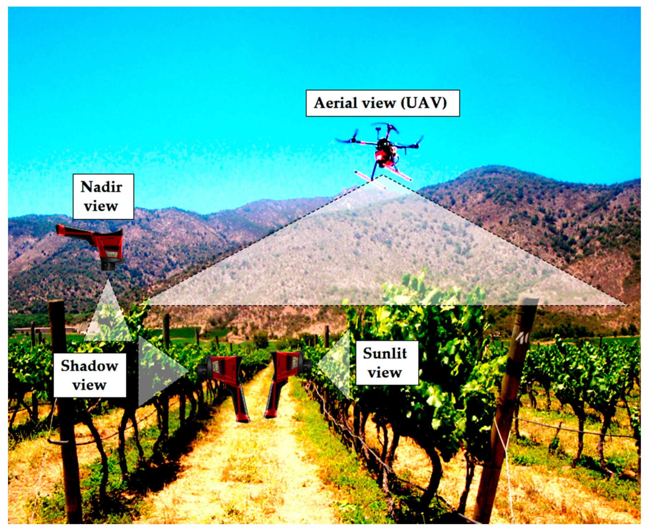
2.6. Canopy Zones and Views

The vine canopy was separated into three main zones (Figure 1): (i) sunlit zone, which was the west row side and which had direct solar radiation above the surface after midday when the measurements were carried out; (ii) shaded zone, which was the east row side with diffuse solar radiation over the surface at measurement time; and (iii) nadir zone, which was the top position of the canopy and had direct solar radiation during the whole day. Lateral (sunlit and shadow view) and nadir thermal images were taken manually with a handheld thermal camera. Aerial thermal images were taken with a thermal camera mounted on a UAV. Sunlit and shadow view images were taken at 1.5 m from the canopy, nadir view images were taken at 0.8 m above the canopy using a ladder over vine rows. Aerial images were recorded at 60 m above ground level (AGL). Ground-based image size was less than 1 m2 and has a resolution less than 1 cm2 per pixel, while each aerial image covered an area of approximately 397 m2 with a resolution of 36 cm2 per pixel.

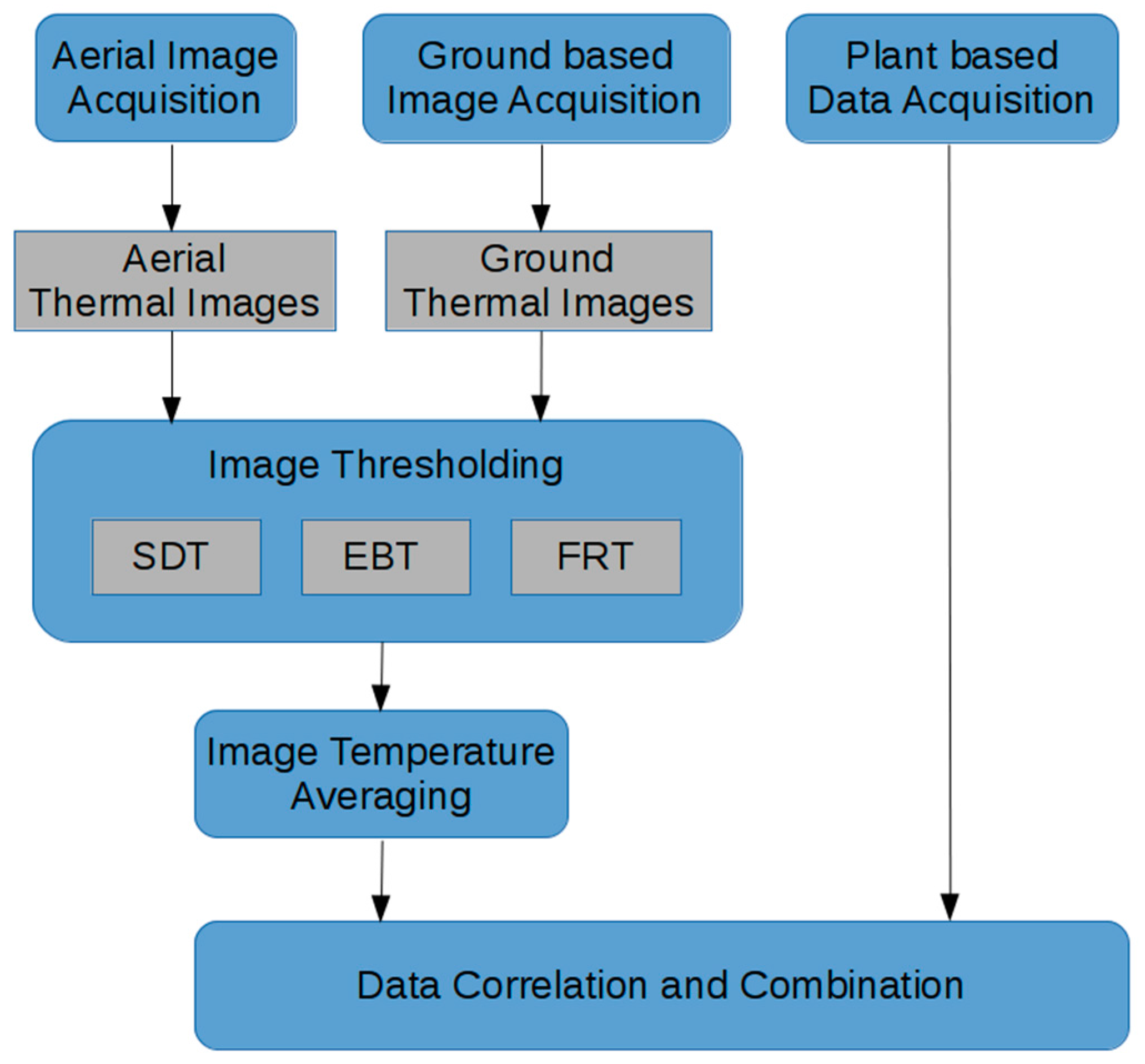
2.7. Image Analysis Processing

All thermal images were post-processed with the proprietary software IrAnalyzer (Wuhan Guide Infrared Co., Ltd., Wuhan, China) to extract temperature data for each treatment considering the specific parameter of emissivity, distance to the object, and measurements of Ta and RH. Then, aerial thermal image data files were converted to Tagged Image File Format (TIFF) with a 16-bit decimal pixel depth using a customized code written in MATLAB® (The Mathworks Inc., Natick, MA, USA), then stitched together using the freely available Image Composite Editor software (ICE version 1.4.4, Microsoft Research, Redmond, WA, USA) to create a mosaic of the experimental plot. To ensure the thermal mosaics created by ICE software did not distort the imagery during the stitching process, segments of imagery from the mosaic were compared with the same segments found in the pre-processed imagery. Calculating the difference between the average temperature values of the pixels in the extracted segments showed negligible differences and, hence, did not generate significant differences in the analysis. The size of the sample was less than the width of the vines and the length of one plant (40 cm × 60 cm) (Figure 2). Thermal markers clearly visible in the thermal mosaic were added to the study area and are aligned with each plant studied. It was not necessary to geo-reference the image since the thermal markers were sufficient for identifying ground-based measurement locations. The thermal mosaic was used only to extract temperature values for the individual treatments. Finally, from each thermal mosaic, two samples of each treatment were extracted manually using MATLAB® code (Figure 2). This MATLAB® code provided a simple graphical interface so that a fixed size segment of pixels (20 × 30 pixels) related to a particular treatment could be extracted by simply selecting the area of interest. Given the selected pixels, the program facilitated the automatic calculation of various statistics, such as minimum, maximum, and median temperatures, as well as the standard deviation of the filtered and unfiltered image. Finally, the program calculated a value for the CWSI for a given segment of pixels selected. A diagram of the methodology used in the study is presented in Figure 3.

Thresholding Approaches

All thermal data files were filtered using a custom program written in MATLAB®. Three different methods were used to determine the upper and lower baseline temperature values, which were used to exclude the non-leaf material.
(1)
Standard deviation technique (SDT): In this technique we used the thermal data file with its unfiltered mean temperature (Tnf) and standard deviation (SD). In each thermal data file the lower temperature was obtained by subtracting a specific multiplier of SD from Tnf and an upper temperature adding another specific multiplier of SD from Tnf. The averages of lower and upper temperatures were calculated to estimate threshold temperature from each batch for a particular date. Specific multiplier values used for each canopy side were estimated using a relationship with threshold values obtained with the methodology described in Field Reference Temperature (see below).
(2)
Energy balance technique (EBT): In this case, temperature threshold values were determined using Equations (2) and (3) described below [23]:
T wet   =   T a + r HR × r aW × γ × R ni ρ a × C p × [ γ × ( r a W ) + Δ × r HR ] r HR × VPD γ × ( r a W ) + Δ × r HR
T dry   =   T a + r HR × R ni ρ a × C p
where, Ta is the air temperature (°C), rHR is the resistance to the radiative heat transfer (s∙m−1), raW is the boundary layer resistance for water vapor (s∙m−1), γ is the psychometric constant (Pa∙K−1), Rni is the net isothermal radiation (W∙m−2), ρa is the density of the air (Kg∙m−3), Cp is the specific heat of air (J∙kg−1∙K−1), and Δ is the slope of the saturation vapor pressure curve (Pa∙K−1). Ancillary information was obtained from an automatic micro-climatic station located near the experimental plot (described in Section 2.4). In this study, net isothermal radiation (Rni) was assumed equal to the net radiation [30,31]. Net radiation (W∙m−2), air temperature (°C), relative humidity (%), and wind velocity (m∙s−1) were used to estimate upper and lower temperatures. This method enabled the estimation of threshold temperatures for each acquisition image time.
(3)
Field reference temperature technique (FRT): This technique was proposed by Jones et al. [21]. Two mature and non-detached leaves were selected from canopy side (sunlit and shaded zone) to obtain upper and lower baseline temperatures. One leaf was painted with a solution of water and detergent (dish-washing soap) to obtain a Twet reference and the other leaf was painted with liquid petroleum jelly (Vaseline) to obtain a Tdry reference. Reference values from sunlit view were used for images captured from nadir view. These threshold temperatures were obtained with IrAnalyzer software (Wuhan Guide Infrared Co., Ltd., Wuhan, China) selecting an area of interest for reference leaves.

2.8. Statistical Analysis

Differences between means of plant-based variables (gs, and Ψstem) were assessed by one-way ANOVA and Tukey’s honestly significant difference (HSD) multiple comparison method using InfoStat software (Student version, InfoStat, Universidad Nacional de Córdoba, Córdoba, Argentina), p-values less than 0.05 were taken to indicate statistically significant differences. Moreover, the evaluation included a linear regression analysis between plant-based variables and the CWSIs obtained from different sides of the canopy. The t-test to evaluate the null hypothesis was to intercept equal to zero and slope equal to unity at the 95% confidence level (i.e., α = 0.05). Additionally, linear relationships between different options of CWSI values and plant-based variables were evaluated using the root mean square error (RMSE) and mean absolute error (MAE).

3. Results

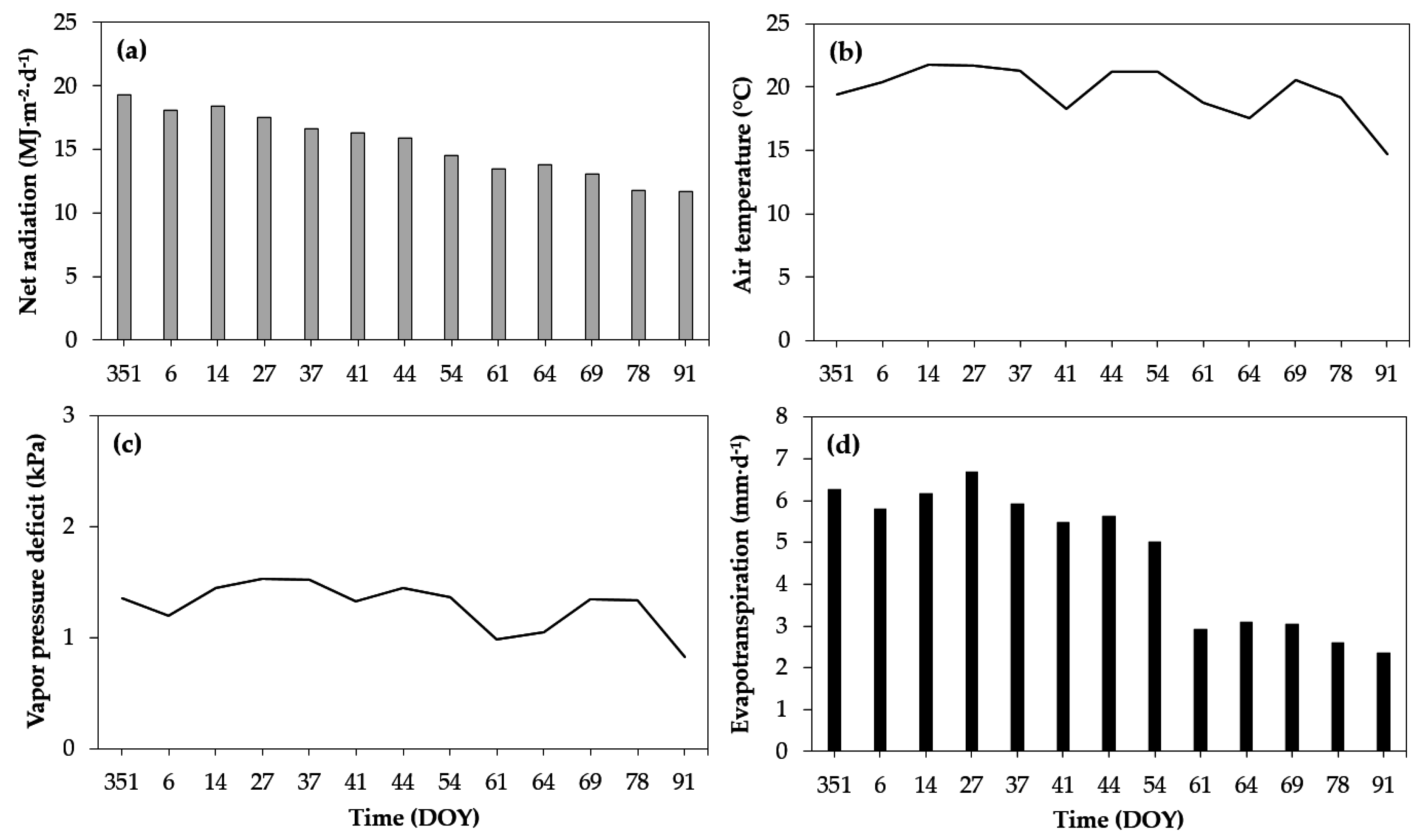
3.1. Description of Climatic Conditions

The climatic conditions during the study period were, in general, dry and hot (Figure 4). Values of daily mean air temperature were similar for the study days, ranging from 14.7–21.8 °C. Similar patterns were presented for relative humidity (RH) and maximum vapor pressure deficit (VPDmax) with average daily values 60.3% and 3.57 kPa, respectively. The net radiation (Rn) was quite stable, with values of 19.3 MJ∙m−2∙day−1 at the beginning of summer and decreasing slowly to 11.7 MJ∙m−2∙day−1 at the end of summer. In general, wind speed (Ws) values were similar during the study. During the thermal acquisition period (around midday) Ws values were lower than 2 m∙s−1. Only three days presented Ws values over 2 m∙s−1 (DOY 351 (2.10 m∙s−1), 6 (2.18 m∙s−1), and 27 (3.01 m∙s−1)). Finally, during the study period, daily reference evapotranspiration (ETo) slowly fell from 6.27 mm∙day−1 (DOY 351) to almost 2 mm∙day−1 (DOY 91). ETo fell strongly on DOY 61, falling 2 mm∙day−1 with respect to the ETo of the previous week.

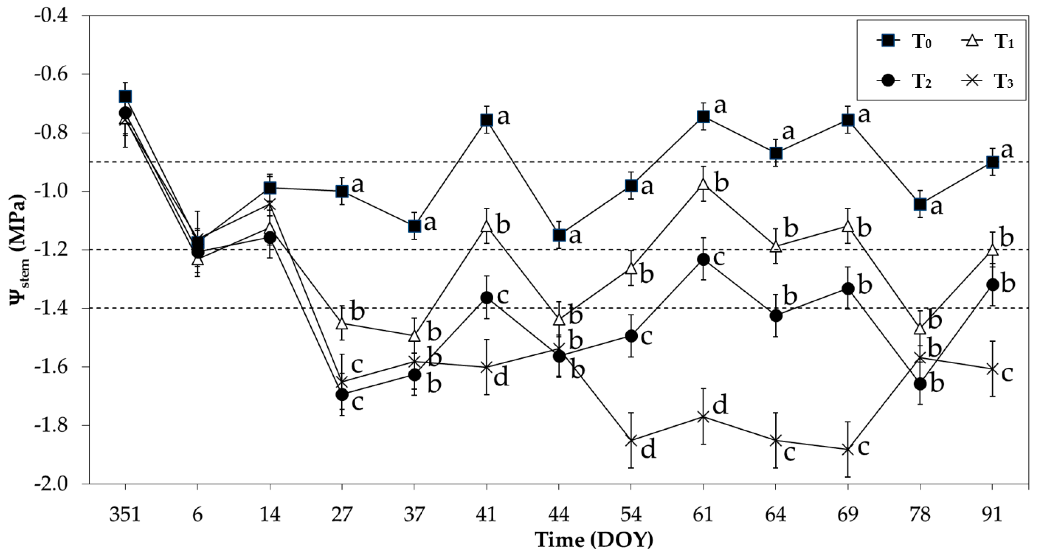
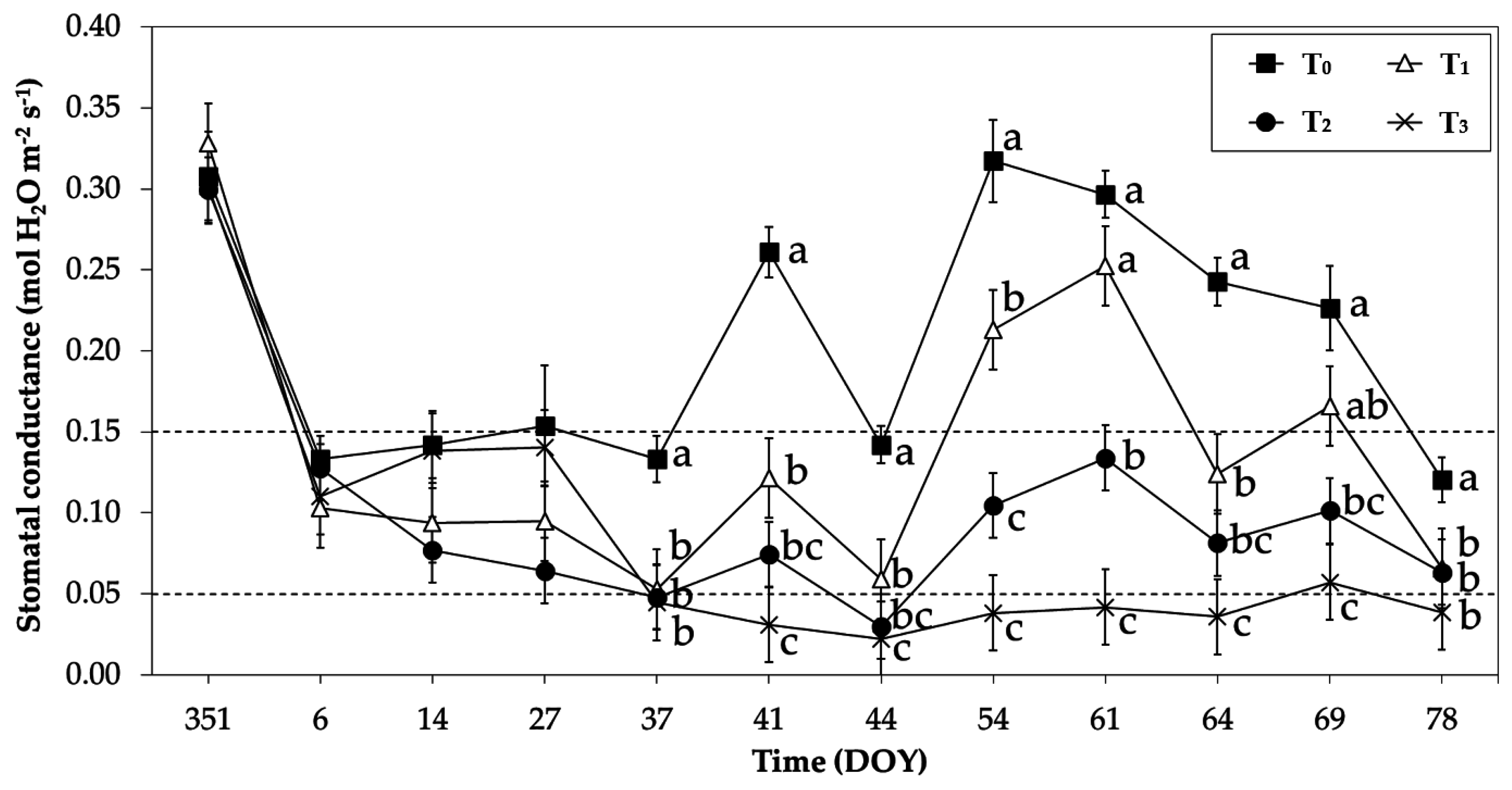
3.2. Results of Plant-Based Variables

The initial conditions for this experiment showed similar Ψstem values with an average of −0.73 MPa for all treatments. Statistical differences between treatments started from DOY 27 (Figure 5). After that, all treatments maintained statistical differences. DOYs 41, 54, and 61 showed statistical differences between all treatments for Ψstem, while DOYs 27, 37, 44, 61, 69, 78, and 91 showed statistical differences between at least two treatments (moderate and severe water stress) (Figure 5). In this regard Choné et al. [28], Sibille et al. [32], Van Leeuwen et al. [27], and Williams and Araujo [33] indicated that midday Ψstem values over −0.8 MPa correspond to grapevines without water stress, between −0.8 to −1.4 MPa correspond to moderate water stress, and lower than −1.4 MPa are grapevines under severe water stress.
In the case of gs, significant differences between treatments started from DOY37, where T0 treatment maintained, in general, over 0.15 mol H2O∙m−2∙s−1. T3 remained under 0.05 mol H2O∙m−2∙s−1, like the most water stressed treatment, and T1 and T2 remained constant in almost all measurement days between 0.15 and 0.05 mol H2O∙m−2∙s−1, except for DOYs 54 and 61, when T1 was close to T0 (Figure 6). Similar levels of gs were found by Cifre et al. [34], Grant et al. [16], and Jara-Rojas et al. [35], where well-watered vines had over 0.15 mol H2O∙m−2∙s−1, vines under moderate water stress were between 0.05 and 0.15 mol H2O∙m−2∙s−1, and below 0.05 mol H2O∙m−2∙s−1 were vines under severe water stress. The leaf temperature (Tleaf) was registered with the thermocouple placed inside the leaf chamber of the infrared gas analyzer (LI-6400, LI-COR Inc., Lincoln, NB, USA). The leaves had an average temperature of 36.6 °C (±2.4 °C). Variations of Tleaf were small between repetitions (±1 °C). Maximum variations of Tleaf were registered between T0 and T3 with values around 5 °C during the period of maximum atmospheric demand (DOY 54 to DOY 64). The relationship between Ψstem and gs was consistent for all treatments during the study days.

3.3. Results of Thresholding Approaches

Table 2 shows a description of CWSI values for each treatment and combination between the canopy zone and thresholding technique during the whole study period. Over 300 data values were used for each combination, except for aerial combinations where less data were used because only eight flights were carried out during the study period. For most of combinations, CWSI mean values for T0 were less than 0.5. In the case of the standard deviation, values around 0.2 were calculated for all combinations, except for AER1 and AER2, which showed values less than 0.1.

3.4. Relationship between CWSIs and Plant-Based Variables

Table 3 shows the coefficient of determination (r2), RMSE and MAE values for each prediction obtained from DOY 37 to 69 using linear regression analysis. During this period, statistical differences between irrigation treatments were registered (see details in Table 4).
Results obtained with the SDT showed that the shadow zone had the best prediction for Ψstem and gs. The sunlit zone had the lowest r2 value for both plant-based variables. In the case of the results obtained with the FRT, it can be seen that SHAD3 had the highest r2 for all canopy zones. The AER3 zone showed the lowest r2, RMSE, and MAE values of the three zones. Results obtained with EBT showed that the r2 of the sunlit and shadow zones were around 0.34 and 0.50 for Ψstem and gs, respectively. The nadir zone with EBT showed the best performance with r2 values of 0.40 for Ψstem and 0.57 for gs. In this case the RMSE values were 0.28 MPa and 0.073 mol H2O∙m−2∙s−1 for Ψstem and gs, respectively. The RMSE and MAE values were similar for all combinations. RMSE were roughly 0.3 MPa and 0.08 mol H2O∙m−2∙s−1 and MAE were roughly 0.23 MPa and 0.06 mol H2O∙m−2∙s−1.
Table 4 shows the coefficient of determination for the comparisons of the CWSI versus Ψstem and gs for each measurement day. Slope and intercept for all predictions of Ψstem and gs were similar in all combinations. In general, slopes were not different from 1 and the intercept was equal to 0, except in the cases where the sunlit side was complemented with SDT and FRT, where the intercept was significantly different to 0. The best results were obtained from DOY 37 until DOY 69 presenting the highest r2 values. Weak relationships between CWSI and plant-based variables were found from DOYs 351, 6, 14, 27, and 64. On the other hand, DOY 44 achieved smaller r2 for all combinations compared with the other measurement dates. This effect could be explained due to a decrease of soil moisture in the vineyard plot, as a consequence of malfunction of the irrigation system during this period. This trend is reasonable due to the differences between stressed and non-stressed treatments showed by Ψstem and gs, which was small compared to other days. r2 of AER2 for Ψstem was the only significant difference on DOY 27, but this did not show statistical significance on DOY 44, while the other combinations showed good relationships with plant-based variables for this particular day.

4. Discussion

The results of three thresholding approaches used to separate the leaf material temperature from the non-leaf material were similar between sunlit and shadow canopy sides, but were different between thresholding approaches. Results obtained with the EBT showed that CWSIs from the sunlit side were higher than CWSIs from the shadow side; however, results obtained with SDT and FRT showed that CWSIs from the shadow side were higher than CWSIs from the sunlit side. This trend of SDT and FRT can be explained due to the use of an underestimated upper threshold temperature by the FRT and a lower threshold temperature overestimated by the SDT in comparison with threshold temperature values used by the EBT.
Thermal data from the sunlit and shadow sides were used to compare the performance of the techniques in the lateral imagery that contained large amounts of vegetation without air or soil components. The SDT detected around 70% of the leaf material from each thermal image (standard deviation over 25%), and FRT showed to be the most restrictive approach due to it filtering a large range of temperature values, especially in the case of the shadow side, with only 39% of the leaf material correctly identified, and 70% in the case of the sunlit side. The EBT was able to discriminate over 95% of the leaf material with a low standard deviation (less than 10%) for the sunlit and shadow views (data not shown). Upper threshold temperatures of the FRT were, in most cases, the lowest values of the three approaches. In the case of the SDT, they also exhibited the highest values of lower threshold temperature of the three techniques (data not shown). Both FRT and SDT could be sources of errors in threshold temperature estimation when compared with the threshold temperature of the EBT. These differences can be explained by the methodology used to obtain the threshold temperature values: (i) threshold temperature values measured in the field showed a greater variability between measured plants. This effect can be explained by the variation in the angle of the measured leaves and gs variance within the leaf causing temperature variations, as suggested by Leinonen and Jones [36]; (ii) SDT was calibrated with values used by the FRT filter for sunlit and shadow canopy sides, since nadir and sunlit sides were similar for both filters; and (iii) in the case of the EBM filter, threshold temperature values were obtained with ancillary weather variables for each image time.
In general terms, CWSI mean values for T0 (full irrigation treatment) were less than 0.5 for most of the combinations analyzed (Table 2). Studies about the use of the CWSI as an indicator of water stress have indicated that plants in a good water condition show CWSI values under 0.5 and plants under water stress had CWSI values over 0.5 in olive orchards [37,38] and vineyards [26,39]. The CWSI was shown to be effective for detecting stress during the period of maximum atmospheric demand. From DOY 37 to 69, the CWSI was able to find statistical differences between T0 and the other stressed treatments. Under the no-water stress period, the CWSI did not show statistical differences for most combinations. These conditions were present at the beginning of the season, when plants are under non-water stress conditions, and at the end of season near to harvest, when plants were close to senescence conditions [26,39].
It can be seen in Table 3 and Table 4 that the CWSI can estimate the gs better than the Ψstem showing higher values of r2 in most of cases. This is validated by Möller et al. [26] and Baluja et al. [18] who found similar results in grapevines of cv. Merlot and Tempranillo, respectively. Berni et al. [37] and Ben-Gal et al. [38] found better correlation for gs in olives than Ψstem. Moreover, Ballester et al. [8] found higher r2 for relative transpiration and sap flow with gs than Ψstem.
On the other hand, some studies have found better adjustments for analytical CWSIs than empirical CWSIs obtained from reference leaves. Ben-Gal et al. [38] found higher r2 for the comparison between CWSIs obtained with equations proposed by Jones [23] with values of stomatal resistance and stem water potential in olives. However, Agam et al. [31] indicated that the empirical threshold temperature had a better performance for estimating water stress in olives than the methodology proposed by Jones [23] and Berni et al. [37] using climatic data. However, Baluja et al. [18] found similar results from CWSIs obtained with climatic data and CWSIs obtained with reference surface temperatures.
In this study, results of sunlit and shadow zones showed differences depending on the SDT and FRT approach used, but were similar in the case of the EBT. This can be explained due to the EBM filter using ancillary information from a weather station, while FRT and SDT used specific information from each side of the canopy. For this reason, the EBT presents some advantages over the FRT approach due to the only requirement being access to the climatic information to calculate the threshold temperature values while the FRT needs more work to obtain the same temperature values. The differences between sunlit and shadow zones with FRT and SDM coincided with those obtained by Jones et al. [21], who found that the shadow side of the canopy was particularly appropriate for row or tree crops. In the case of nadir view, the results obtained with the EBT and FRT filters coincided with those obtained by Ballester et al. [40], who found that significant differences were detected in the nadir zone between stressed and non-stressed plants when lateral images did not detect differences between them. However, Ochagavia [19] found that r2 values in vineyards with temperature values recorded from the lateral canopy side were higher than temperature values measured from the nadir position. Lower r2 values of aerial CWSIs (AER1, AER2, and AER3), in comparison with CWSIs obtained from nadir zones, could be explained due to the resolution of the imagery. From high spatial resolution imagery, it is easier to extract leaf-material temperatures from the thermal image, but with lower spatial resolution some leaf temperatures are mixed with non-leaf materials in some pixels of the thermal images [36]. For future studies, the height of flight should be studied so as to obtain better correlation with ground-based variables as, at lower heights, it is assumed that the relationship would be more accurately identified (Ψstem and gs).
The low values of r2 obtained in the beginning and the end of the grapevine growing season could be explained due to specific plant conditions of the vineyard. Some authors proposed that phenological stages could have affected the CWSI accuracy of water stress prediction. Möller et al. [26] found that in vineyards at the end of the growing season, leaves were in a senescence condition and may not have been representative of complete canopy conditions, and Bellvert et al. [39] found differences between varieties and the phenological stage in vineyards, as well as peach and nectarine orchards [41].
In general, the CWSI values obtained using EBT and FRT had the highest correlation coefficients with Ψstem and gs. Regarding the simplicity, the FRT would be recommendable because it is easy to calculate. However, with this technique the determination of Tdry and Twet has some methodological aspects related to the preparation and reading of reference leaves in the thermal images that can limit robustness for monitoring large areas, specifically under conditions of significant environmental variation. Meanwhile, EBT requires a set of microclimate measurements to obtain the temperature threshold values, which are not always available in commercial vineyards. In this regards, the use of SDT can be a good alternative when there are limitations in obtaining microclimatic information, because it uses only information from images. Additionally, this technique is easy to implement in the field, because the use of reference images is not necessary. Regarding the canopy zone analysis, in general, NAD and SHAD ground-based positions had the highest correlation coefficients with Ψstem and gs during the period of maximum atmospheric demand. The apparent low robustness of the SUN zone to the other ground-based positions may relate to the greater temperature variability of this zone. On the other hand, the aerial view obtained by the UAV has, in general, a lower correlation coefficient than the ground-based positions; however, this method has many advantages from a practical point of view. The use of UAVs make it possible to monitor large vineyards with high spatial and temporal resolution rapidly and for a very low operational cost. Additionally, there are several low-cost and user-friendly aerial platforms on the market today. The cost of suitable thermal cameras is dropping rapidly due to better technology and higher demand. However, the use of UAVs are limited by governmental regulations, weather conditions (wind and rain primarily), and difficulties for flying over agricultural areas with rugged terrain geography.

5. Conclusions

Our results indicate that the use of thermal imaging (aerial and ground-based) is a feasible tool for remotely monitoring grapevine water status. Nevertheless, it is necessary to take into consideration the effect of selecting canopy zones and thresholding approaches used to analyze thermal images. In this study, the CWSIs derived from all combinations of thresholding approaches and canopy zones were able to discriminate between vines under water stress and vines in good water conditions. Moreover, results showed that the CWSI obtained from different canopy zones in a commercial vineyard trained on VSP changed depending mostly on the methodology used to extract the temperature from the imagery and to calculate the thermal index.
The estimation of Ψstem and gs using CWSI values obtained from sunlit and shaded zones were clearly different for FRT and SDM approaches, where the shaded zone allowed the estimation of water stress conditions with more accuracy than the CWSI values obtained from the sunlit canopy zone. The EBT approach did not show higher differences of water stress prediction between sunlit and shaded zones or aerial CWSI. Nadir images processed by EBT showed the best performance for determining plant-based variables Ψstem and gs, reaching coefficients of determination (r2) of 0.73 and 0.82, respectively.
The best relationships between the CWSIs and plant-based variables were registered during the period of maximum atmospheric demand (near veraison from DOY 37 until DOY 69) with significant correlations registered for all methods. During the period with non-water stress conditions, the CWSI did not show a good relationship with measured plant-based variables. Therefore, the seasonal effect needs to be taken into account to improve water stress prediction using thermal imaging.
Finally, in order to determine the most adequate canopy zone and thermal imagery thresholding, it is important to take into consideration the level of agreement with plant-based variables. Additionally, other factors, such as how easily images can be acquired, the need of microclimate data, and the size of the monitoring zone, should be considered.

Acknowledgments

This study was supported by the Chilean government through the project FONDECYT DE INICIACION N° 11130601, and by the Universidad de Talca through the research program “Adaptation of Agriculture to Climate Change (A2C2)”. We thank the Academic Writing Center at Programa de Idiomas at Universidad de Talca.

Author Contributions

Carlos Poblete-Echeverría, conceived and guided the study, performed the interpretation of the results and reviewed and edited the manuscript. Daniel Sepulveda Reyes wrote the paper, conducted the field experiments and performed the data analysis. Samuel Ortega-Farías collaborated in article writing and provided suggestions for the study. Mauricio Zuñiga collaborated in the field experiments and article writing. Benjamin Ingram and Matthew Bardeen participated in the article writing and data analysis.

Conflicts of Interest

The authors declare no conflict of interest.

References

  1. Jones, H.G. Irrigation scheduling: Advantages and pitfalls of plant-based methods. J. Exp. Bot. 2004, 55, 2427–2436. [Google Scholar] [CrossRef] [PubMed]
  2. McCarthy, M.G. The effect of transient water deficit on berry development of cv. Shiraz (Vitis vinifera L.). Aust. J. Grape Wine Res. 1997, 3, 2–8. [Google Scholar] [CrossRef]
  3. Peterlunger, E.; Sivilotti, P.; Bonetto, C.; Paladin, M. Water stress induces changes in polyphenol concentration in Merlot grapes and wines. Riv. Vitic. Enol. 2002, 1, 51–66. [Google Scholar]
  4. Acevedo, C.; Ortega-Farías, S.; Moreno, Y.; Córdova, F. Effects of different levels of water application in pre- and post-veraison on must composition and wine color (cv. Cabernet sauvignon). ISHS Acta Hortic. 2004, 664, 483–489. [Google Scholar] [CrossRef]
  5. Meza, L.; Corso, S.; Soza, S. Gestión del Riesgo de Sequía y Otros Eventos Climáticos Extremos en Chile; Organización de las Naciones Unidas para la Alimentación y la Agricultura (FAO): Santiago, Chile, 2010; p. 117. [Google Scholar]
  6. Romero, P.; Fernandez-Fernandez, J.I.; Martinez-Cutillas, A. Physiological thresholds for efficient regulated deficit-irrigation management in winegrapes grown under semiarid conditions. Am. J. Enol. Vitic. 2010, 61, 300–312. [Google Scholar]
  7. Fuentes, S.; Bei, R.; Pech, J.; Tyerman, S. Computational water stress indices obtained from thermal image analysis of grapevine canopies. Irrig. Sci. 2012, 30, 523–536. [Google Scholar] [CrossRef]
  8. Ballester, C.; Castel, J.; Jiménez-Bello, M.A.; Castel, J.R.; Intrigliolo, D.S. Thermographic measurement of canopy temperature is a useful tool for predicting water deficit effects on fruit weight in citrus trees. Agric. Water Manag. 2013, 122, 1–6. [Google Scholar] [CrossRef]
  9. Costa, J.M.; Grant, O.M.; Chaves, M.M. Thermography to explore plant–environment interactions. J. Exp. Bot. 2013, 64, 3937–3949. [Google Scholar] [CrossRef] [PubMed]
  10. Jones, H.G. Use of thermography for quantitative studies of spatial and temporal variation of stomatal conductance over leaf surfaces. Plant Cell Environ. 1999, 22, 1043–1055. [Google Scholar] [CrossRef]
  11. Poblete-Echeverría, C.; Ortega-Farías, S.; Zuñiga, M.; Lobos, G.A.; Romero, S.; Estrada, F.; Fuentes, S. Use of infrared thermography on canopies as indicator of water stress in ‘Arbequina’ olive orchards. ISHS Acta Hortic. 2014, 1057, 399–403. [Google Scholar] [CrossRef]
  12. Poblete-Echeverría, C.; Sepulveda-Reyes, D.; Ortega-Farias, S.; Zuñiga, M.; Fuentes, S. Plant water stress detection based on aerial and terrestrial infrared thermography: A study case from vineyard and olive orchard. ISHS Acta Hortic. 2016, 1112, 141–146. [Google Scholar] [CrossRef]
  13. Idso, S.B.; Jackson, R.D.; Pinter, P.J., Jr.; Reginato, R.J.; Hatfield, J.L. Normalizing the stress-degree-day parameter for environmental variability. Agric. Meteorol. 1981, 24, 45–55. [Google Scholar] [CrossRef]
  14. Jackson, R.D.; Idso, S.B.; Reginato, R.J.; Pinter, P.J. Canopy temperature as a crop water stress indicator. Water Resour. Res. 1981, 17, 1133–1138. [Google Scholar] [CrossRef]
  15. Wang, X.; Yang, W.; Wheaton, A.; Cooley, N.; Moran, B. Automated canopy temperature estimation via infrared thermography: A first step towards automated plant water stress monitoring. Comput. Electron. Agric. 2010, 73, 74–83. [Google Scholar] [CrossRef]
  16. Grant, O.M.; Tronina, L.; Jones, H.G.; Chaves, M.M. Exploring thermal imaging variables for the detection of stress responses in grapevine under different irrigation regimes. J. Exp. Bot. 2007, 58, 815–825. [Google Scholar] [CrossRef] [PubMed]
  17. Jones, H.G.; Serraj, R.; Loveys, B.R.; Xiong, L.; Wheaton, A.; Price, A.H. Thermal infrared imaging of crop canopies for the remote diagnosis and quantification of plant responses to water stress in the field. Funct. Plant Biol. 2009, 36, 978–989. [Google Scholar] [CrossRef]
  18. Baluja, J.; Diago, M.; Balda, P.; Zorer, R.; Meggio, F.; Morales, F.; Tardaguila, J. Assessment of vineyard water status variability by thermal and multispectral imagery using an unmanned aerial vehicle (UAV). Irrig. Sci. 2012, 30, 511–522. [Google Scholar] [CrossRef]
  19. Ochagavía, H. Application of Thermography for the Assessment of Vineyard Water Status. Master’s Thesis, Universidad de la Rioja, Logroño, España, 2012. [Google Scholar]
  20. Zarco-Tejada, P.J.; Gonzalez-Dugo, V.; Berni, J.A.J. Fluorescence, temperature and narrow-band indices acquired from a UAV platform for water stress detection using a micro-hyperspectral imager and a thermal camera. Remote Sens. Environ. 2012, 117, 322–337. [Google Scholar] [CrossRef]
  21. Jones, H.G.; Stoll, M.; Santos, T.; de Sousa, C.; Chaves, M.M.; Grant, O.M. Use of infrared thermography for monitoring stomatal closure in the field: Application to grapevine. J. Exp. Bot. 2002, 53, 2249–2260. [Google Scholar] [CrossRef] [PubMed]
  22. Idso, S.B.; Reginato, R.J.; Jackson, R.D.; Pinter, P.J., Jr. Foliage and air temperatures: Evidence for a dynamic “equivalence point”. Agric. Meteorol. 1981, 24, 223–226. [Google Scholar] [CrossRef]
  23. Jones, H.G. Use of infrared thermometry for estimation of stomatal conductance as a possible aid to irrigation scheduling. Agric. For. Meteorol. 1999, 95, 139–149. [Google Scholar] [CrossRef]
  24. Reinert, S.; Bögelein, R.; Thomas, F.M. Use of thermal imaging to determine leaf conductance along a canopy gradient in European beech (Fagus sylvatica). Tree Physiol. 2012, 32, 294–302. [Google Scholar] [CrossRef] [PubMed]
  25. Pou, A.; Diago, M.P.; Medrano, H.; Baluja, J.; Tardaguila, J. Validation of thermal indices for water status identification in grapevine. Agric. Water Manag. 2014, 134, 60–72. [Google Scholar] [CrossRef]
  26. Moller, M.; Alchanatis, V.; Cohen, Y.; Meron, M.; Tsipris, J.; Naor, A.; Ostrovsky, V.; Sprintsin, M.; Cohen, S. Use of thermal and visible imagery for estimating crop water status of irrigated grapevine. J. Exp. Bot. 2007, 58, 827–838. [Google Scholar] [CrossRef] [PubMed]
  27. Van Leeuwen, C.; Tregoat, O.; Chone, X.; Bois, B.; Pernet, D.; Gaudillere, J.P. Vine water status is a key factor in grape ripening and vintage quality for red bordeaux wine. How can it be assessed for vineyard management purposes? J. Int. Sci. Vigne Vin 2009, 43, 121–134. [Google Scholar] [CrossRef]
  28. Chone, X.; van Leeuwen, C.; Dubourdieu, D.; Gaudillere, J.P. Stem water potential is a sensitive indicator of grapevine water status. Ann. Bot. 2001, 87, 477–483. [Google Scholar] [CrossRef]
  29. Allen, R.G.; Pereira, L.S.; Raes, D.; Smith, M. Crop Evapotranspiration-Guidelines for Computing Crop Water Requirements—FAO Irrigation and Drainage Paper 56; Food and Agriculture Organization (FAO): Rome, Italy, 1998. [Google Scholar]
  30. Leinonen, I.; Grant, O.M.; Tagliavia, C.P.P.; Chaves, M.M.; Jones, H.G. Estimating stomatal conductance with thermal imagery. Plant. Cell Environ. 2006, 29, 1508–1518. [Google Scholar] [CrossRef] [PubMed]
  31. Agam, N.; Cohen, Y.; Alchanatis, V.; Ben-Gal, A. How sensitive is the CWSI to changes in solar radiation? Int. J. Remote Sens. 2013, 34, 6109–6120. [Google Scholar] [CrossRef]
  32. Sibille, I.; Ojeda, H.; Prieto, J.; Maldonado, S.; Lacapere, J.N.; Carbonneau, A. Relation between the values of three pressure chamber modalities (midday leaf, midday stem and predawn water potential) of 4 grapevine cultivars in drought situation of the southern of France. Applications for the irrigation control. In Proceedings of the XVth International Symposium (GESCO), Porec, Croacia, 20–23 June 2007; pp. 685–695.
  33. Williams, L.E.; Araujo, F.J. Correlations among Predawn Leaf, Midday Leaf, and Midday Stem Water Potential and their Correlations with other Measures of Soil and Plant Water Status in Vitis vinifera. J. Am. Soc. Hortic. Sci. 2002, 127, 448–454. [Google Scholar]
  34. Cifre, J.; Bota, J.; Escalona, J.M.; Medrano, H.; Flexas, J. Physiological tools for irrigation scheduling in grapevine (Vitis vinifera L.): An open gate to improve water-use efficiency? Agric. Ecosyst. Environ. 2005, 106, 159–170. [Google Scholar]
  35. Jara-Rojas, F.; Ortega-Farías, S.; Valdés-Gómez, H.; Acevedo-Opazo, C. Gas exchange relations of ungrafted grapevines (cv. Carménère) growing under irrigated field conditions. S. Afr. J. Enol. Vitic. 2015, 36, 231–242. [Google Scholar]
  36. Leinonen, I.; Jones, H.G. Combining thermal and visible imagery for estimating canopy temperature and identifying plant stress. J. Exp. Bot. 2004, 55, 1423–1431. [Google Scholar] [CrossRef] [PubMed]
  37. Berni, J.A.J.; Zarco-Tejada, P.J.; Sepulcre-Canto, G.; Fereres, E.; Villalobos, F. Mapping canopy conductance and CWSI in olive orchards using high resolution thermal remote sensing imagery. Remote Sens. Environ. 2009, 113, 2380–2388. [Google Scholar] [CrossRef]
  38. Ben-Gal, A.; Agam, N.; Alchanatis, V.; Cohen, Y.; Yermiyahu, U.; Zipori, I.; Presnov, E.; Sprintsin, M.; Dag, A. Evaluating water stress in irrigated olives: Correlation of soil water status, tree water status, and thermal imagery. Irrig. Sci. 2009, 27, 367–376. [Google Scholar] [CrossRef]
  39. Bellvert, J.; Marsal, J.; Girona, J.; Zarco-Tejada, P.J. Seasonal evolution of crop water stress index in grapevine varieties determined with high-resolution remote sensing thermal imagery. Irrig. Sci. 2014, 33, 81–93. [Google Scholar] [CrossRef]
  40. Ballester, C.; Jiménez-Bello, M.A.; Castel, J.R.; Intrigliolo, D.S. Usefulness of thermography for plant water stress detection in citrus and persimmon trees. Agric. For. Meteorol. 2013, 168, 120–129. [Google Scholar] [CrossRef]
  41. Bellvert, J.; Marsal, J.; Girona, J.; Gonzalez-Dugo, V.; Fereres, E.; Ustin, S.L.; Zarco-Tejada, P.J. Airborne thermal imagery to detect the seasonal evolution of crop water status in peach, nectarine and Saturn peach orchards. Remote Sens. 2016, 8, 39–55. [Google Scholar] [CrossRef]
Figure 1. Schematic layout of vineyard canopy zones analyzed in the experiment: aerial view (60 m height) and three ground based positions (sunlit, shadow, and nadir view).
Remotesensing 08 00822 g001
Figure 2. Thermal mosaic used to extract temperature values of each treatment in the experimental plot for UAV thermal imaging acquisition.
Remotesensing 08 00822 g002
Figure 3. Diagram of the methodology used in the study.
Remotesensing 08 00822 g003
Figure 4. Net radiation (a); Daily mean air temperature (b); Daily mean vapor pressure deficit (c); and Reference evapotranspiration (d) measured in the field during the study period.
Remotesensing 08 00822 g004
Figure 5. Stem water potential (Ψstem) of vines under different water stress conditions during the study period. Vertical bars indicate standard error (n = 4). Equal letters for means at identical DOY indicate no statistical differences by Tukey’s honestly significant difference (HSD) multiple comparison method (α = 0.05).
Remotesensing 08 00822 g005
Figure 6. Stomatal conductance to water vapor (gs) of vines under different water stress conditions during the study period. Vertical bars indicate standard error (n = 4). Equal letters for means at identical DOY indicate no statistical differences by Tukey’s honestly significant difference (HSD) multiple comparison method (α = 0.05).
Remotesensing 08 00822 g006
Table 1. Thresholds of stem water potential defined for irrigation treatments.
TreatmentsWater Stress Conditions* Stem Water Potential (MPa)
T0Null-Slight0 to −0.8
T1Slight-Moderate−0.8 to −1.1
T2Moderate-Severe−1.1 to −1.4
T3SevereLess than −1.4
* Modify from [27].
Table 2. CWSI values obtained using different combinations (canopy zones–thresholding approaches) for the entire dataset during the study period.
ZoneTechniqueCodenTreatments
T0T1T2T3
NADIRSDTNAD13510.18 (0.09)0.29 (0.15)0.33 (0.13)0.44 (0.18)
SUNLITSDTSUN13840.20 (0.13)0.31 (0.15)0.31 (0.16)0.43 (0.18)
SHADOWSDTSHAD13650.47 (0.24)0.66 (0.25)0.70 (0.22)0.83 (0.16)
AERIALSDTAER12480.21 (0.06)0.24 (0.06)0.29 (0.07)0.36 (0.08)
NADIREBTNAD23510.35 (0.18)0.46 (0.18)0.51 (0.17)0.59 (0.16)
SUNLITEBTSUN23840.37 (0.18)0.49 (0.20)0.49 (0.18)0.57 (0.19)
SHADOWEBTSHAD23820.27 (0.16)0.38 (0.19)0.40 (0.17)0.49 (0.17)
AERIALEBTAER22560.52 (0.09)0.58 (0.11)0.62 (0.10)0.69 (0.09)
NADIRFRTNAD33480.44 (0.20)0.58 (0.23)0.63 (0.21)0.72 (0.20)
SUNLITFRTSUN33670.50 (0.21)0.62 (0.22)0.63 (0.20)0.73 (0.18)
SHADOWFRTSHAD33090.67 (0.25)0.74 (0.24)0.80 (0.21)0.91 (0.11)
AERIALFRTAER32480.49 (0.15)0.58 (0.16)0.63 (0.17)0.69 (0.14)
Note: Code is the name used for each combination; n is the size of data set; T0, T1, T2, and T3 are the irrigation treatments. Values in brackets represent the standard deviation. NADIR, SUNLIT, SHADOW, and AERIAL are ground based nadir, sunlit, and shadow views, and aerial nadir view, respectively. SDT is the thermal standard deviation technique; EBT is the thermal energy balance technique; FRT is the thermal field reference temperature technique.
Table 3. Coefficient of determination (r2), root mean square error (RMSE), and mean absolute error (MAE) from different predictions with CWSI versus plant-based variables (Ψstem and gs).
Statistical ParametersNAD1SUN1SHAD1AER1NAD2SUN2SHAD2AER2NAD3SUN3SHAD3AER3
Ψstem
r20.340.320.460.360.400.360.330.220.260.210.360.20
RMSE0.300.320.290.250.280.310.310.300.300.320.300.27
MAE0.230.260.230.190.220.240.230.240.230.262.470.22
gs
r20.330.300.420.260.570.520.510.280.430.380.470.27
RMSE0.0840.0890.0820.0750.0730.0750.0770.0780.0770.0800.0770.074
MAE0.0650.0710.0650.0520.0530.0570.0600.0600.0600.0630.0600.052
Note: statistical significance (p-values < 0.05).
Table 4. Coefficient of determination (r2) between Ψstem and gs versus CWSI obtained from different thresholding approaches on each measurement date.
DOYNAD1SUN1SHAD1AER1NAD2SUN2SHAD2AER2NAD3SUN3SHAD3AER3
Ψstem
351n.s.n.s.n.s.-n.s.n.s.n.s.-n.s.n.s.n.s.-
6n.s.0.35n.s.-n.s.n.s.n.s.-n.s.n.s.n.s.-
140.130.11n.s.-n.s.0.13n.s.-n.s.0.120.16-
27-n.s.n.s.0.59-n.s.n.s.0.50-n.s.n.s.0.55
370.440.530.63-0.650.660.63-0.680.650.68-
410.740.610.760.680.820.720.780.680.710.700.760.55
440.280.310.37n.s.0.420.510.38n.s.0.420.470.40n.s.
540.700.620.700.460.770.680.800.530.770.680.720.36
610.300.210.310.280.390.290.170.160.390.300.310.24
640.270.240.570.480.330.320.380.610.350.330.430.61
690.220.270.220.570.250.360.140.520.270.350.170.61
78n.s.n.s.n.s.0.190.15n.s.n.s.0.340.13n.s.n.s.0.39
91n.s.0.13n.s.-n.s.0.230.13-n.s.0.22n.s.-
gs
351n.s.n.s.n.s.-n.s.n.s.n.s.-n.s.n.s.n.s.-
6n.s.n.s.n.s.-n.s.n.s.n.s.-n.s.n.s.n.s.-
14n.s.n.s.n.s.-n.s.n.s.n.s.-n.s.n.s.n.s.-
27-n.s.n.s.n.s.-n.s.n.s.n.s.-n.s.0.15n.s.
370.490.510.68-0.620.630.66-0.600.460.71-
410.630.560.700.710.730.670.770.750.580.600.690.54
440.510.540.430.240.590.540.460.220.650.570.320.40
540.620.400.370.480.660.480.510.320.640.490.380.41
610.400.280.260.320.480.390.320.170.480.400.280.26
640.290.370.640.450.430.590.670.480.430.610.540.61
690.330.150.120.310.330.260.200.260.320.24n.s.0.47
780.17n.s.0.170.230.14n.s.n.s.0.720.13n.s.n.s.0.51
Note: statistical significance (p-value < 0.05); n.s. is not statistical significance (Tukey’s honestly significant difference (HSD) multiple comparison method (α = 0.05)).

