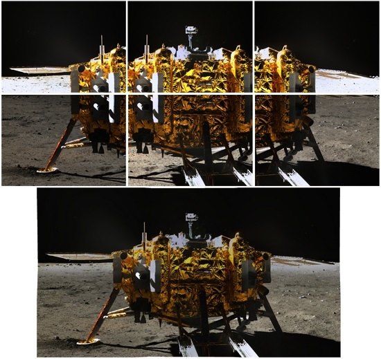
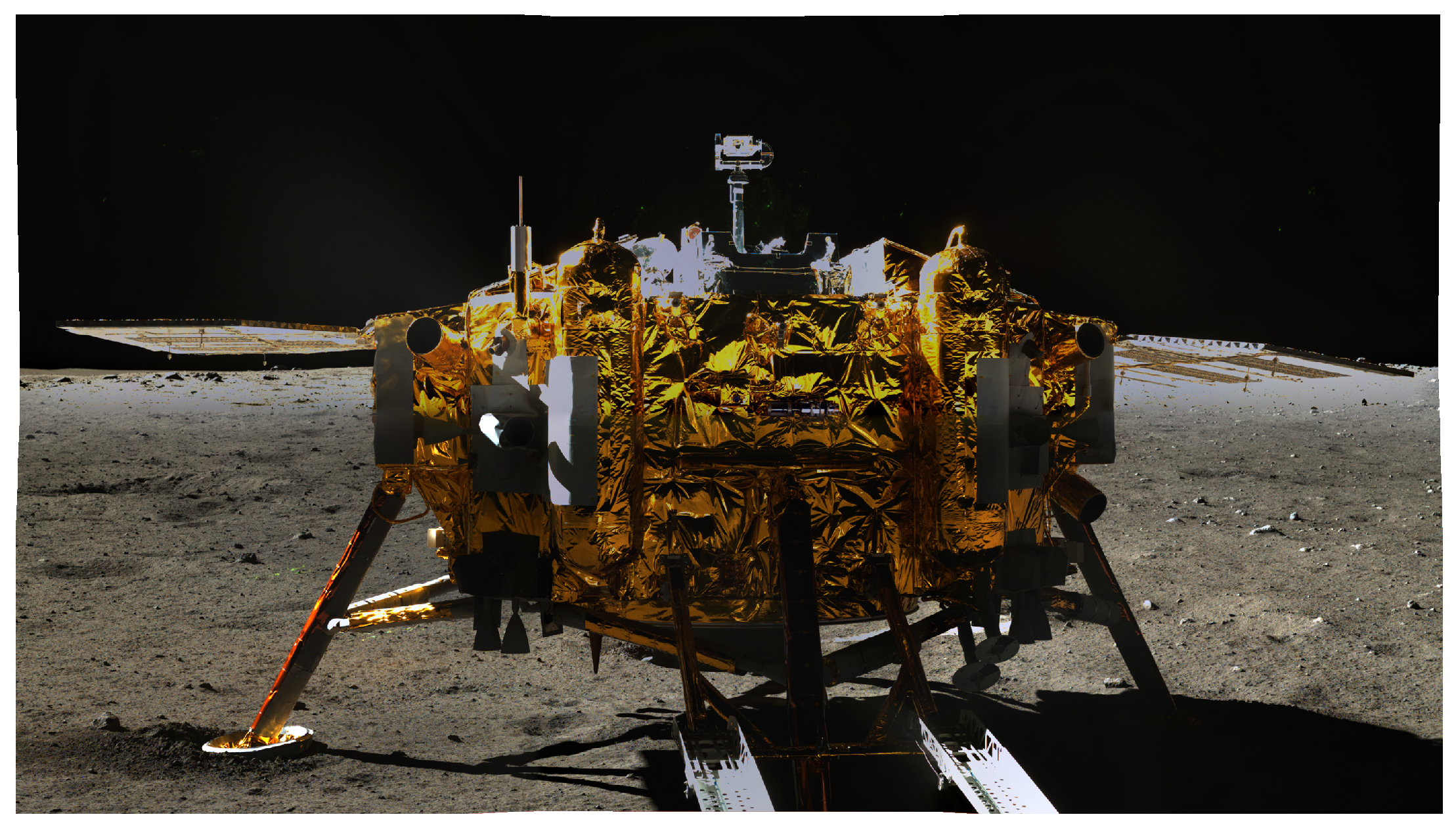
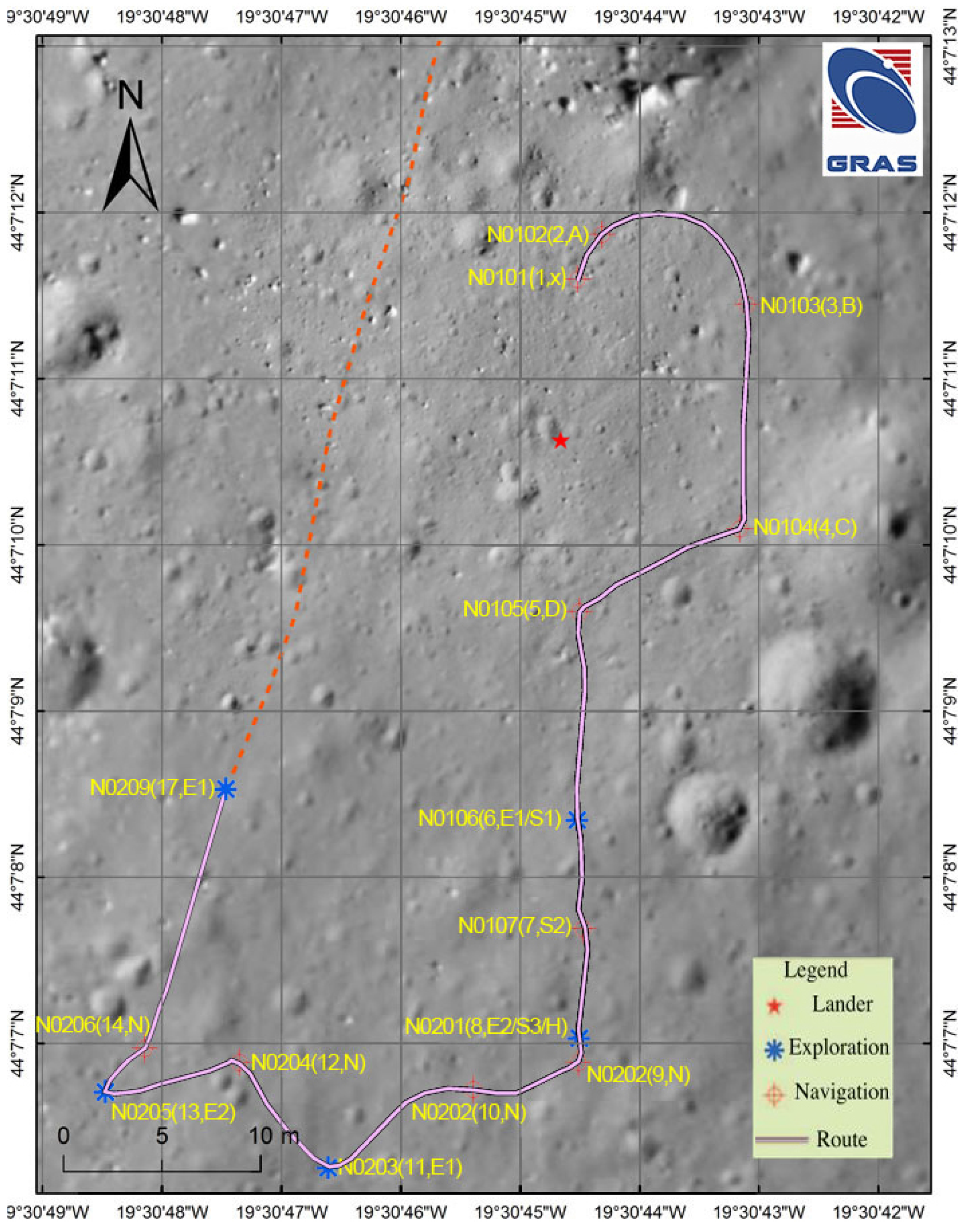
Panoramic Mosaics from Chang’E-3 PCAM Images at Point A

Abstract

This paper presents a unique approach for panoramic mosaics based on Moon surface images from the Chang’E-3 (CE-3) mission, with consideration of the exposure time and external illumination changes in CE-3 Panoramic Camera (PCAM) imaging. The engineering implementation involves algorithms of image feature points extraction by using Speed-Up Robust Features (SURF), and a newly defined measure is used to obtain the corresponding points in feature matching. Then, the transformation matrix is calculated and optimized between adjacent images by the Levenberg–Marquardt algorithm. Finally, an image is reconstructed by using a fade-in-fade-out method based on linear interpolation to achieve a seamless mosaic. The developed algorithm has been tested with CE-3 PCAM images at Point A (one of the rover sites where the rover is separated from the lander). This approach has produced accurate mosaics from CE-3 PCAM images, as is indicated by the value of the Peak Signal to Noise Ratio (PSNR), which is greater than 31 dB between the overlapped region of the images before and after fusion.

1. Introduction

The CE-3 lunar surface exploration mission, including a lander and a rover (named Yutu), was launched at 17:30 (UTC), 1 December 2013. The lander carries four scientific payloads, the Terrain Camera (TCAM), Landing Camera (LCAM), Extreme Ultraviolet Camera (EUVC) and Moon-based Ultraviolet Telescope (MUVT), while Yutu (the rover) was equipped with the Panoramic Camera (PCAM), Lunar Penetrating Radar (LPR), Visible/Near-Infrared Imaging Spectrometer (VNIS) and Active Particle-induced X-ray Spectrometer (APXS) [1]. Mounted on the top of the mast of the Yutu rover, the PCAM is composed of two cameras (separated by a 270 mm baseline) with identical specifications, which is capable of acquiring 3D imagery of the lunar surface for the purposes of interpreting the terrain with geological features and structures, and understanding craters near the landing area. The mosaic processing presented in this paper is intended to achieve the designated scientific objectives.

Based on the principle of binocular stereo vision, the CE-3 PCAM (Panoramic Camera) can acquire 3D imagery of the lunar surface. The focal length of each camera is about 50 mm with a field of view (FOV) of ${19.7}^{\circ }\times {14.5}^{\circ }$. The image sensor is a Complementary Metal Oxide Semiconductor (CMOS) chip, and

Table 1. Technical Indices of CE-3 PCAM (Panoramic Camera).

Character	Value
Sensor mode	IA-G3 DALSA
Pixel numbers	2352 × 1728
Pixel size ($\mathsf{\mu }$m)	7.4
Frame frequency	62 $fps$
Spectral range (nm)	420∼700
Color	(R, G, B)
Baseline (mm)	270
Imaging mode	Color or Panchromatic mode
Normal imaging distance (m)	3∼∞
Effective pixel numbers	1176 × 864 (Color mode); 2352 × 1728 (Panchromatic mode)
FOV	19.7${}^{\circ }$× 14.5${}^{\circ }$
Focal length (mm)	50
Quantitative value (bit)	10
S/N (dB)	≥40 (maximum); ≥30 (albedo: 0.09; solar elevation: 30${}^{\circ }$)
Optical system static MTF	0.33
Weight (kg)	0.64

FOV: field of view. MTF: modulation transfer function.

gives technical indices of the CE-3 PCAM. CE-3 soft-landed on 13:11 (UTC), 14 December 2013. The landing site $(44.{12}^{\circ }$N, $19.{50}^{\circ }$W) is located in Mare Imbrium, about 40 km south of the crater Laplace F. After departure from the lander, Yutu rover started working (Figure 1).

Image mosaicking is a process to obtain a panoramic image with a large view angle from sequences of images which are overlapped. Over the last two decades, image mosaicking has found practical applications in solving many real world problems across diverse fields, such as space exploration [2,3,4,5], virtual reality [6], motion analysis [7] and remotely sensed image processing [8,9]. There are four major steps for image mosaicking, i.e., geometric correction, pre-processing, registration, and fusion. Image registration is the primary difficulty and it is the basis of image fusion. In the research papers, methods for image registration are broadly classified into two categories: feature-based [10,11,12,13] and region-based [14,15]. Feature-based registration uses features such as edges [16], contours or corner points [17] to find matches between adjacent images. Region-based registration methods calculate the gray-level statistics of the overlap between adjacent images, and then apply designated similarity measures for image registration. In this study, we take the following facts into account. First, the lunar surface has simple terrain features and a lack of textural features. Second, the lunar surface image has a narrow dynamic range and a low contrast. Third, influenced by the solar elevation and the low albedo, image observations of the lunar surface have obvious differences under disparate light conditions. Therefore region-based registration methods are not suitable in this study, but feature-based registration methods are considered, although textural features are limited.

The study aims to develop an effective method to achieve the panoramic mosaics of CE-3 PCAM images. One of the contributions of this study is a novel image matching strategy. Firstly, initial matching is achieved based on the nearest neighbor distance ratio (NNDR) [18]. Then, the Euclidean distance of the Speed-Up Robust Features (SURF) descriptor is used as the measure to obtain the correct matches.

The rest of the paper is structured as follows. Section 2 describes the new method for panoramic mosaics and the novel image matching methodology. Section 3 demonstrates the experiments of feature detection, matching and image fusion. In Section 4, we present the panoramic mosaicking results from CE-3 PCAM images at Point A. Finally, the paper presents conclusions in Section 5.

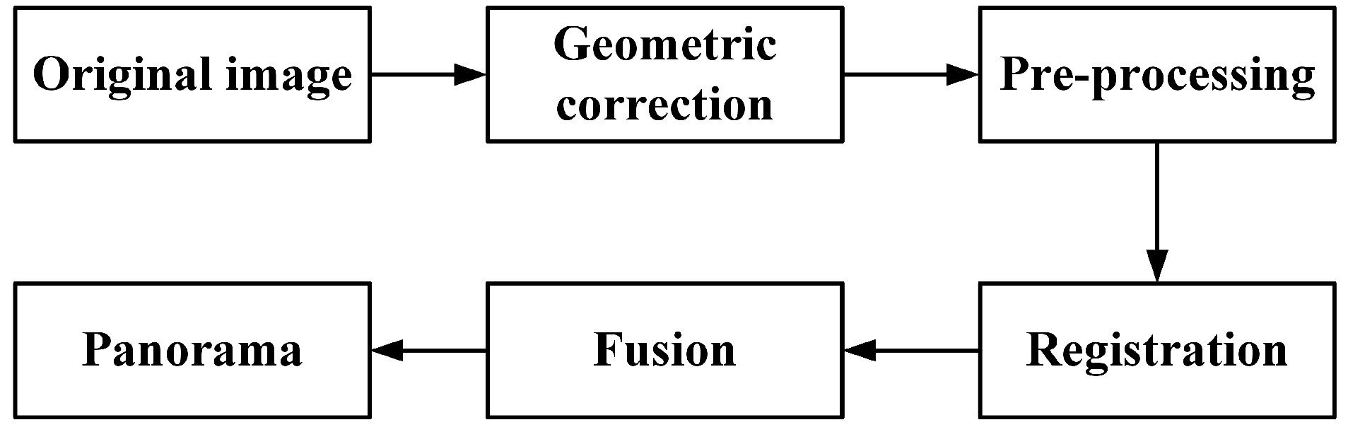
2. Methodology Used in Panoramic Mosaics

As shown in Figure 2, the developed algorithm consists of four main steps. With the input of original images, a method based on circular markers [19] is used to achieve geometric correction; pre-processing is then put into force; a novel image matching strategy is applied for obtaining the corresponding points, and then—to establish the transformation matrix between adjacent images—combined with a fade-in-fade-out fusion method based on linear interpolation to obtain the panorama. The details of the method are discussed in the following sections.

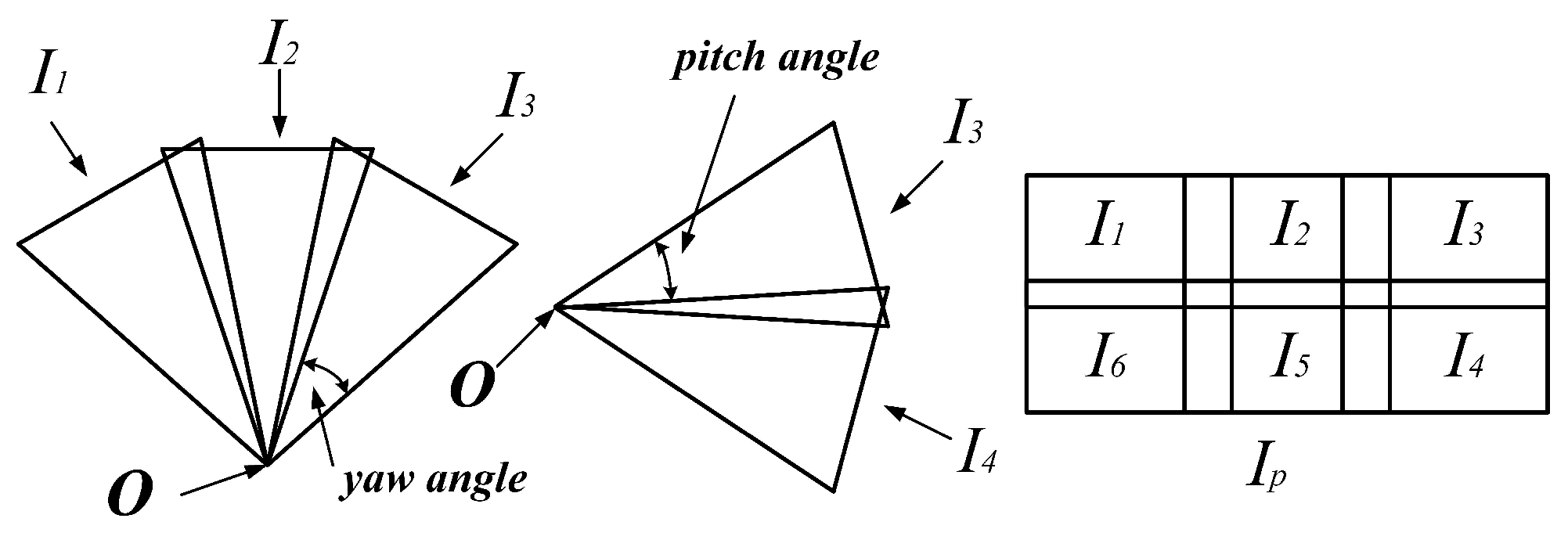
2.1. Geometric Correction

Geometric correction is meant for decreasing matching errors introduced by geometric distortion of the camera. The Brown model [20,21,22,23] that is most commonly used to describe lens distortion can be written as

$$\left\{\begin{array}{c}\begin{array}{cc}\hfill x_u=& (x_d-x_0)(1+k_1{r}_d^2+k_2{r}_d^4+k_3{r}_d^6+...)\hfill \\ & +(1+p_3{r}_d^2+...)\left\{p_1\left[r_d^2+2{(x_d-x_0)}^2\right]+2p_2(x_d-x_0)(y_d-y_0)\right\},\hfill \end{array}\hfill \\ \begin{array}{cc}\hfill y_u=& (y_d-y_0)(1+k_1{r}_d^2+k_2{r}_d^4+k_3{r}_d^6+...)\hfill \\ & +(1+p_3{r}_d^2+...)\left\{p_2\left[r_d^2+2{(y_d-y_0)}^2\right]+2p_1(x_d-x_0)(y_d-y_0)\right\},\hfill \end{array}\hfill \end{array}\right.$$

(1)

where $(x_u,y_u)$ and $(x_d,y_d)$ are the corresponding coordinates of an undistorted point and a distorted point in an image, respectively. $r_d$ is the Euclidean distance of the distorted point to the distortion center, $(x_0,y_0)$ is the center of distortion

$$r_d^2={(x_d-x_0)}^2+{(y_d-y_0)}^2.$$

(2)

The Brown model only takes into account radial distortion and decentering distortion, and $x_0$, $y_0$, $k_1$, $k_2$, $k_3$, $p_1,p_2,p_3,...,p_n$ are distortion parameters, which must be estimated from image measurements. To achieve high-accurate estimation of the distortion parameters in the CE-3 PCAM, Ref. [19] added image-sensor-array-deformation parameters into the model as

$$\left\{\begin{array}{c}\begin{array}{cc}\hfill x_u=& (x_d-x_0)(1+k_1{r}_d^2+k_2{r}_d^4+k_3{r}_d^6+...)+b_1(x_d-x_0)+b_2(y_d-y_0)\hfill \\ & +(1+p_3{r}_d^2+...)\left\{p_1\left[r_d^2+2{(x_d-x_0)}^2\right]+2p_2(x_d-x_0)(y_d-y_0)\right\}\hfill \end{array}\hfill \\ \begin{array}{cc}\hfill y_u=& (y_d-y_0)(1+k_1{r}_d^2+k_2{r}_d^4+k_3{r}_d^6+...)+b_2(x_d-x_0)+b_1(y_d-y_0)\hfill \\ & +(1+p_3{r}_d^2+...)\left\{p_2\left[r_d^2+2{(y_d-y_0)}^2\right]+2p_1(x_d-x_0)(y_d-y_0)\right\}\hfill \end{array}\hfill \end{array}\right.$$

(3)

Parameters of CE-3 PCAM, including focus lengths, principal point offset and lens distortions, are obtained from the calibration experiment using the method based on circular markers [19,24]. A large number of circular markers are distributed on the target in matrix form, one of which is taken as the origin of a world coordinate system. Based on the camera model and collinearity of object point, camera origin, and image point, the optimal camera parameters are finalized with a nonlinear optimization method [25], which uses minimizing projection error as the objective function. Results show that the projection error is better than 0.04 pixels [19].

2.2. Pre-Processing

Images of the lunar surface carry unique characteristics reflecting the nature of the terrain in Mare Imbrium, a low contrast and shortage of textural features. In addition, image noise influences feature extraction and matching. The pre-processing addresses the above issues, and enhances signal-to-noise ratio (SNR). CE-3 PCAM has two imaging modes: color mode and panchromatic mode. When the CE-3 PCAM works in the color mode (Table 1), it can observe the state of the lander from color images. Under this circumstance, the PCAM calibration also includes: dark current correction, relative radiation calibration, mode normalization, and color calibration. Dark current is the detector response to null radiation input, and it is a major source of noise in digital imagers [26,27]. It directly influences the contrast of imaging. To eliminate the dark current interference and improve the image contrast, the direct component of the dark current should be subtracted. The relative radiation calibration (flat field correction) aims to eliminate the response inconsistency between pixels. The relative changes of image intensity of the images taken at different working modes (at different exposure time and different gain) should be consistent, hence the need to implement mode normalization. Based on the Bayer color coding principle, the CE-3 PCAM uses a Bayer color filter array (CFA) covering the image sensor to capture color images [28]. As the detector response curve is different from the International Commission on Illumination (CIE) 1931 chromaticity diagram, the color images have unique chromatism. Color calibration is applied to correct the chromatism. After calculating the white balance coefficient and color correction coefficient matrix, a color image is accurately reproduced with true object color.

2.3. Registration

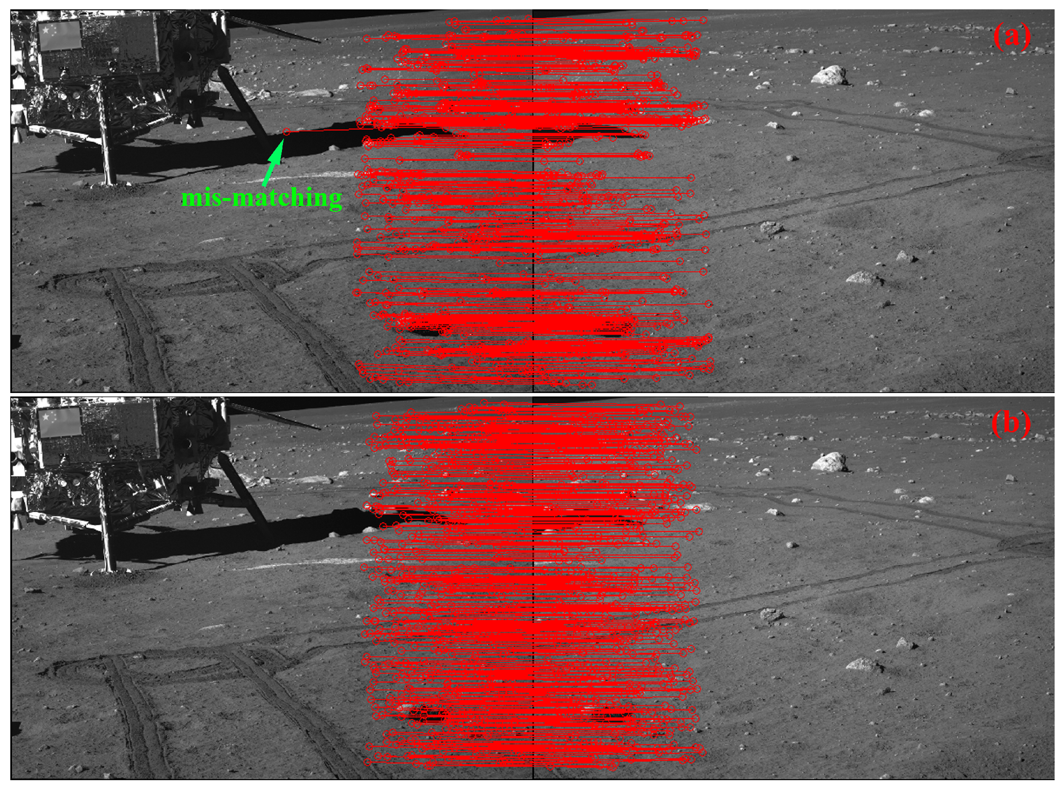
2.3.1. Feature Matching

Feature detection and matching is a fundamental problem in many computer vision applications. A feature in an image here refers to a specific meaningful structure in the image. Features can range from a single pixel to edges and contours, and can be as large as objects in the image. In the past decades, various types of feature detectors and descriptors have been proposed in the research papers [29,30,31,32].

Scale Invariant Feature Transform (SIFT) proposed by Lowe [33], is one of the most popular feature detectors and descriptors. It transforms image data into scale-invariant coordinates relative to local features. In this method, SIFT features are located at scale-space maxima/minima of a difference of Gaussian function. At each feature location, a characteristic scale and orientation are established [34]. Interest points are extracted from the image in two steps. First, the image is repeatedly smoothed using Gaussian filters and subsampled to find images in smaller scales. An image pyramid is constructed with the reference image at the ground level (level 1). Second, interest points are discovered in the $3\times 3\times 3$ neighborhood of any pixel at an intermediate level. These points are obtained from the image points where the difference-of-Gaussians values attain an extrema, both in the spatial domain and the scale level of the Gaussian pyramid [32,33]. SIFT features are invariant under rotation and scale changes, and have better adaptability for affine distortion, change of view point, image noise, and change in illumination.

SURF [35] is a very efficient and robust scale- and rotation-invariant feature detector and descriptor algorithm. It is based on a Hessian matrix, which is generated by convolution of the Gaussian second-order derivative with image pixels. The interest points are extracted by a 3 × 3 × 3 non-maximal suppression on a Gaussian pyramid, followed by interpolation of the maxima of the Hessian matrix [35].

SURF detectors are found on each interest point by orientation assignment and descriptor component analysis. The orientation is assigned by calculating a Haar Wavelet response in x- and y- directions in a circular neighborhood of each interest point. The dominant orientation is found by calculating the sum of orientations. Then, the Wavelet responses in a square region oriented in the dominant orientation provide the SURF descriptors [32,35]. These descriptors are scale and rotation-invariant and are very robust against transformations on images.

SURF is very similar to SIFT and the interest points are extracted in the same way as SIFT, but it is much faster compared to SIFT. This paper uses the SURF algorithm to detect feature points, and a newly defined measure is used to obtain the corresponding points in feature matching. A feature point is represented by a 64-dimensional descriptor vector. Assuming that ${\mathit{X}}^{\mathit{i}}=(x_1^i,x_2^i,...,x_{64}^i)$ and ${\mathit{Y}}^{\mathit{j}}=(y_1^j,y_2^j,...,y_{64}^j)$ represent feature points of two adjacent images, the Euclidean distance (also called ${\mathit{L}}_{\mathbf{2}}$ distance) between ${\mathit{X}}^{\mathit{i}}$ and ${\mathit{Y}}^{\mathit{j}}$ is defined as:

$$D_{ij}=\sqrt{{(x_1^i-y_1^j)}^2+{(x_2^i-y_2^j)}^2+\cdots +{(x_{64}^i-y_{64}^j)}^2}.$$

(4)

The matching strategy is then improved by the following two steps:

First step:

NNDR is applied in the initial matching. ${\mathit{Y}}^{\mathit{a}}$ is the nearest neighbor and ${\mathit{Y}}^{\mathit{b}}$ is the second-nearest neighbor to ${\mathit{X}}^{\mathit{i}}$, if

$$\frac{D_{ia}}{D_{ib}}<thr.$$

(5)

${\mathit{X}}^{\mathit{i}}$ and ${\mathit{Y}}^{\mathit{a}}$ are matched, and $thr$ is the threshold.

Second step:

Normally, false matches still exist after the NNDR based matching. Assume the number of corresponding points obtained from the initial matching is n, sorting these $D_{ij}$ by values (smallest to largest), the smaller the $D_{ij}$, the higher the precision of matching is. Therefore, the first $m(m<n)$ matching points are taken as the correct matches.

Using this strategy, we can get the specified number of correct matches.

2.3.2. Establishment and Optimization of Transformation Matrix

The set of correct matches is used to establish the transformation matrix $\mathit{M}$ between adjacent images. During the PCAM panoramic imaging process, the pitch angle (the rotation angle around the horizontal axis of the mast) changes by ${12}^{\circ }$ between images, while the yaw angle (the rotation angle around the vertical axis of the mast) changes by ${13}^{\circ }$ between images [24]. The panorama is captured by turning PCAM, and a block diagram for the panoramic capture process is illustrated in Figure 3. Thus, the relationship of corresponding points as:

$$\left[\begin{array}{c}{x}_1\\ y_1\\ 1\end{array}\right]={\mathit{M}}_{\mathbf{21}}\left[\begin{array}{c}{x}_2\\ y_2\\ 1\end{array}\right]=\left[\begin{array}{ccc}{m}_1& m_2& m_3\\ m_4& m_5& m_6\\ m_7& m_8& 1\end{array}\right]\left[\begin{array}{c}{x}_2\\ y_2\\ 1\end{array}\right],$$

(6)

where $(x_1,y_1)$ is the coordinate of corresponding points in $I_1$ and $(x_2,y_2)$ is the corresponding coordinate in $I_2$, ${\mathit{M}}_{\mathbf{21}}$ is the transformation matrix between $I_1$ and $I_2$. We wish to resolve the transformation parameters ($m_1$ to $m_8$), so that Equation (6) is rewritten as:

$$\left\{\begin{array}{c}{x}_2{m}_1+y_2{m}_2+m_3-x_1{x}_2{m}_7-x_1{y}_2{m}_8=x_1\hfill \\ x_2{m}_4+y_2{m}_5+m_6-y_1{x}_2{m}_7-y_1{y}_2{m}_8=y_1\hfill \end{array}\right..$$

(7)

Equation (6) gives a single pixel match. More matching points increase the number of equations in Equation (6). At least four matches, each adding two equations in Equation (6), are needed to provide a solvable solution based on the least-squares method. In order to improve precision, this study optimizes the solution by the Levenberg–Marquardt algorithm [25].

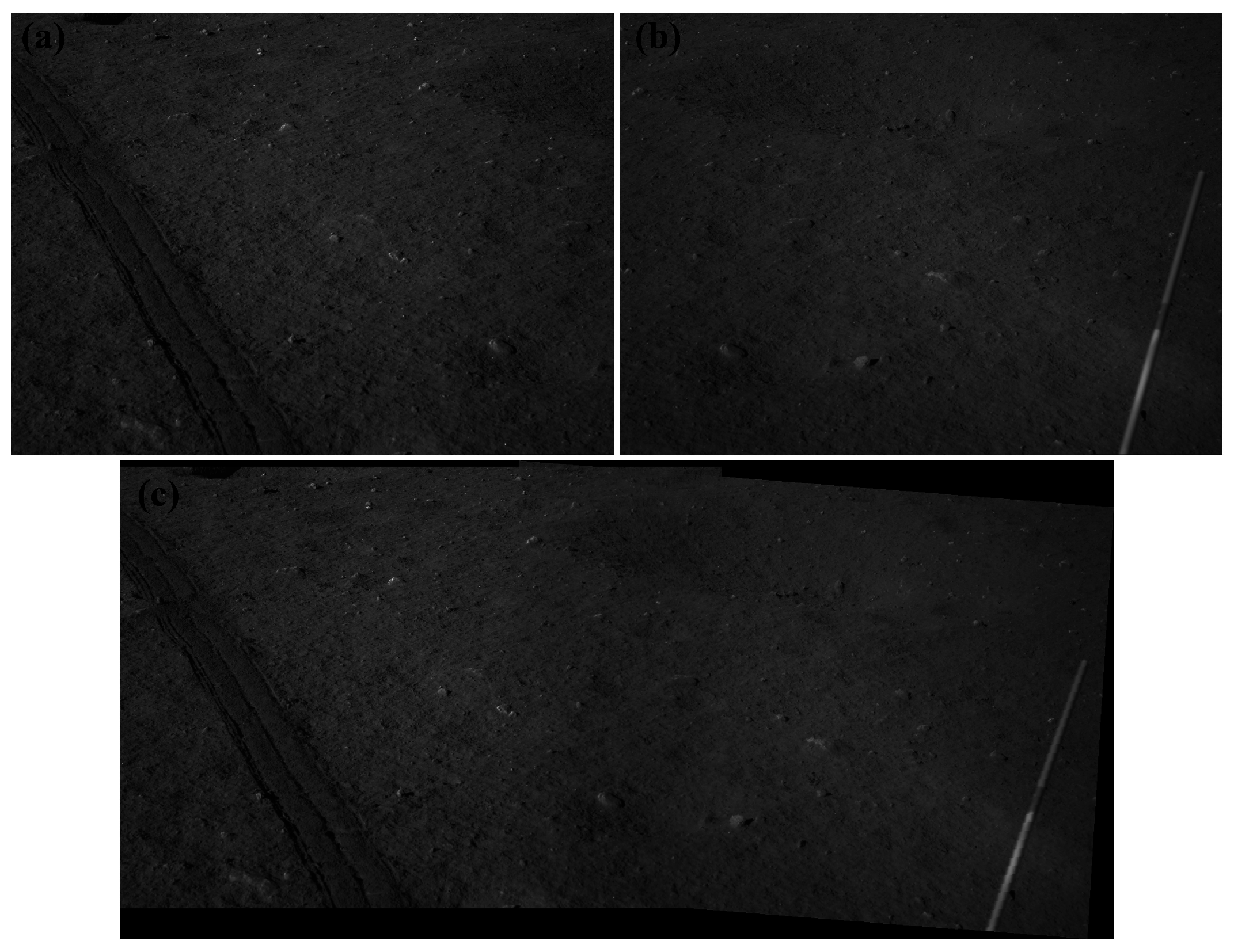
2.4. Fusion of Overlapped Images

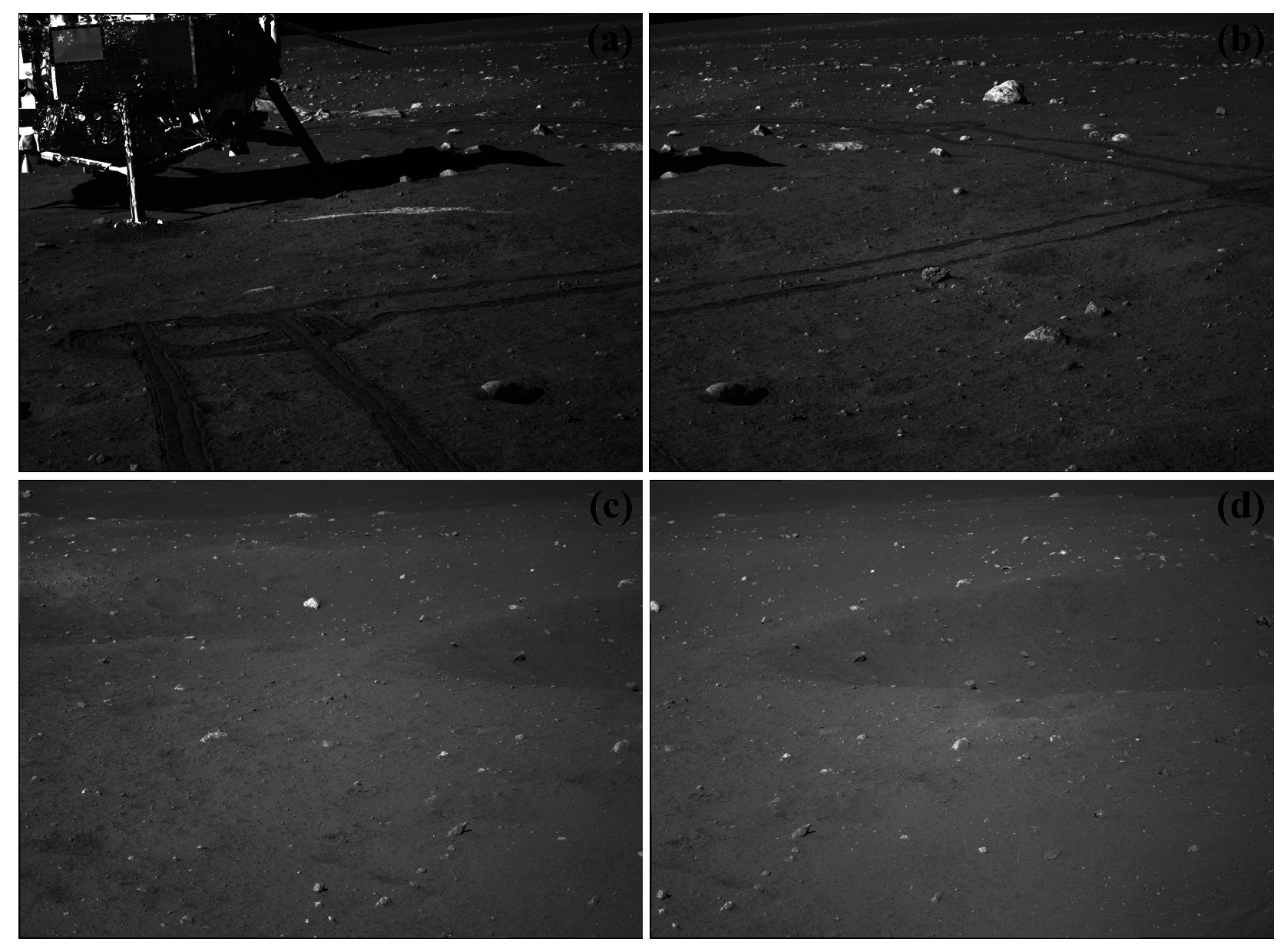
The purpose of image fusion is to keep the individual information of the non-overlapping regions, and smooth the transition of the overlapping region to achieve the seamless mosaic of the image. In this paper, the fade-in-fade-out method based on linear interpolation has been applied to fuse overlapped regions between images. For example, $I_1$, $I_2$ in Figure 3 are two images waiting to be fused, and I is the fused image, so that:

$$I(x,y)=\left\{\begin{array}{c}\begin{array}{cc}\beta I_1(x,y)+(1-\beta )I_2(x,y)& (x,y)\in I_1\cup I_2,\\ I_1(x,y)& (x,y)\in I_1\backslash I_2,\\ I_2(x,y)& (x,y)\in I_2\backslash I_1.\end{array}\hfill \end{array}\right.$$

(8)

β is the fade factor:

$$\beta =\frac{x_{max}-x}{x_{max}-x_{min}},$$

(9)

where $x_{min}$ is the minimum X coordinate of the overlapped region, and $x_{max}$ is the maximum X coordinate of the overlapped region. Similarly, when $I_3$, $I_4$ in Figure 3 are two images waiting to be fused, β is related to the Y-axis projection of the overlapped region. The transformation matrix ${\mathit{M}}_{\mathbf{21}}$ between $I_1$ and $I_2$ can be calculated by Equation (6), and then the solution is optimized by the Levenberg–Marquardt algorithm. Thus, the coordinates of the four corner points in $I_2$ are mapped in the $I_1$ coordinate systems, and thereby the overlapped region can be ensured. $I_2(x,y)$ is gray value at point $(x,y)$ ( or Red-Green-Blue value for the color image) of the projected image of $I_2$.

The method is based on the pixel of the overlapping region, and we performed the fusion incrementally, generated first $I_{12}$ from $I_1$ and $I_2$, and then used $I_{12}$ to fuse with $I_3$. In the course of the projection, a point with full-pixel coordinates in the original image $I_2$ generally corresponds to subpixel coordinates in the projected image, and thus interpolation is necessary. Considering effects and computational costs, this study adopts a bilinear interpolation approach. Then, the fusion processing of the overlapping region went through the whole images row-by-row or column-by-column.

The information loss after images are fused can be quantitatively evaluated using Peak Signal to Noise Ratio ($PSNR$):

$$PSNR=10\times {log}_{10}\left(\frac{{255}^2}{MSE}\right).$$

(10)

$MSE$ is the mean square error between the overlapped region of the images before and after fusion:

$$MSE=\frac{1}{MN}\sum _{x=0}^{M-1}\sum _{y=0}^{N-1}{\left|I_k(x,y)-I_p(x,y)\right|}^2,$$

(11)

where M and N are the length and width of the overlapping region, and $I_k(x,y)$ and $I_p(x,y)$ are gray value (or Red-Green-Blue value for color image) of the overlapped region of the images before and after fusion. There are two $PSNR$ values, and the average of the two values are taken as the final result.

3. Experiments

3.1. Experiments of Feature Matching

To verify the feasibility of the proposed method, we have performed experiments on four images obtained from the CE-3 PCAM. Figure 4 shows the images after the geometric correction and pre-processing. It has to be noted that it is achieved by setting appropriate parameters in both SIFT and SURF algorithms that the number of feature points extracted from Figure 4a is approximately equal from both algorithms. The overall number of feature points is shown in

Table 2. The number of extracted feature points.

Algorithm	a	b	c	d
SIFT	5445	3496	874	753
SURF	4955	4911	3267	2430

SIFT: Scale Invariant Feature Transform. SURF: Speed-Up Robust Features.

. From Section 2, a small number of corresponding points has a negative impact for calculating and optimizing the transformation matrix. It can be seen that the SURF algorithm can cope with the external illumination changes of CE-3 PCAM images and applies to the lunar surface image better than the SIFT algorithm.

The ratio of $D_{ij}$ is used as the measure to implement initial matching. The threshold $thr$ for NNDR changes from $0.7$ to $0.2$, the number of corresponding points from initial matching is shown in

Table 3. Matching results.

$\mathit{thr}$	a–b		c–d
	SIFT	SURF	SIFT	SURF
0.70	890 (F)	786 (F)	242 (F)	573 (F)
0.65	855 (F)	754 (F)	226 (F)	546 (F)
0.60	813 (F)	725 (F)	214 (F)	513 (F)
0.55	767 (F)	682 (F)	198 (T)	471(T)
0.50	716 (F)	636 (F)	182 (T)	411 (T)
0.45	652 (F)	580 (T)	163 (T)	349 (T)
0.40	570 (F)	493 (T)	139 (T)	282 (T)
0.35	474 (F)	388 (T)	111 (T)	211 (T)
0.30	365 (F)	277 (T)	87 (T)	127 (T)
0.25	261 (T)	160 (T)	61 (T)	70 (T)
0.20	151 (T)	75 (T)	35 (T)	35 (T)

F: exist obviously false matches. T: not exist obviously false matches. SIFT: Scale Invariant Feature Transform. SURF: Speed-Up Robust Features.

. As seen from Table 3, the SURF algorithm does not have obvious advantages in the number of corresponding points with the same $thr$ value, whereas it is robust and has a higher accuracy, as shown in Figure 5.

Furthermore, we have conducted experiments only using the SIFT algorithm on 56 images, which were acquired by the CE-3 PCAM on 23 December 2013. To make the process more efficient, $thr$ was set to the same value as the 56 images. First, $thr$ was set to $0.2$, and the results showed that the number of corresponding points is not sufficient, although there are no obviously false matches. A small number of corresponding points has a negative impact for calculating and optimizing the transformation matrix. Then, when $thr$ was $0.4$, the results showed that the number of corresponding points increased, but the false matches obviously increased as well. In order to identify false matches, some research papers employed a RANSAC (RANdom SAmple Consensus) algorithm [36]. We have performed experiments on the same images by using the SURF algorithm with $thr$ set to $0.4$, and the results showed that there were no obviously false matches (see Figure 5b). This paper finally used the SURF algorithm to detect feature points, with $thr$ set to $0.4$ and m (see Section 2.3 for more details) set to 100 for CE-3 PCAM images.

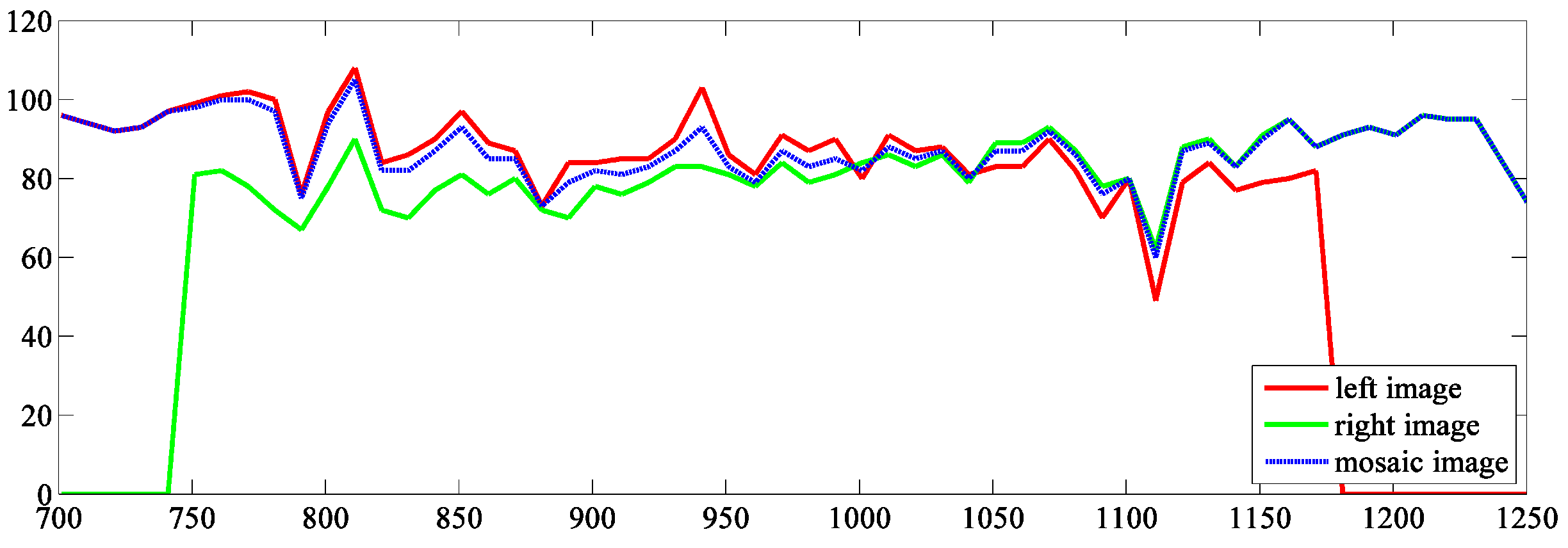
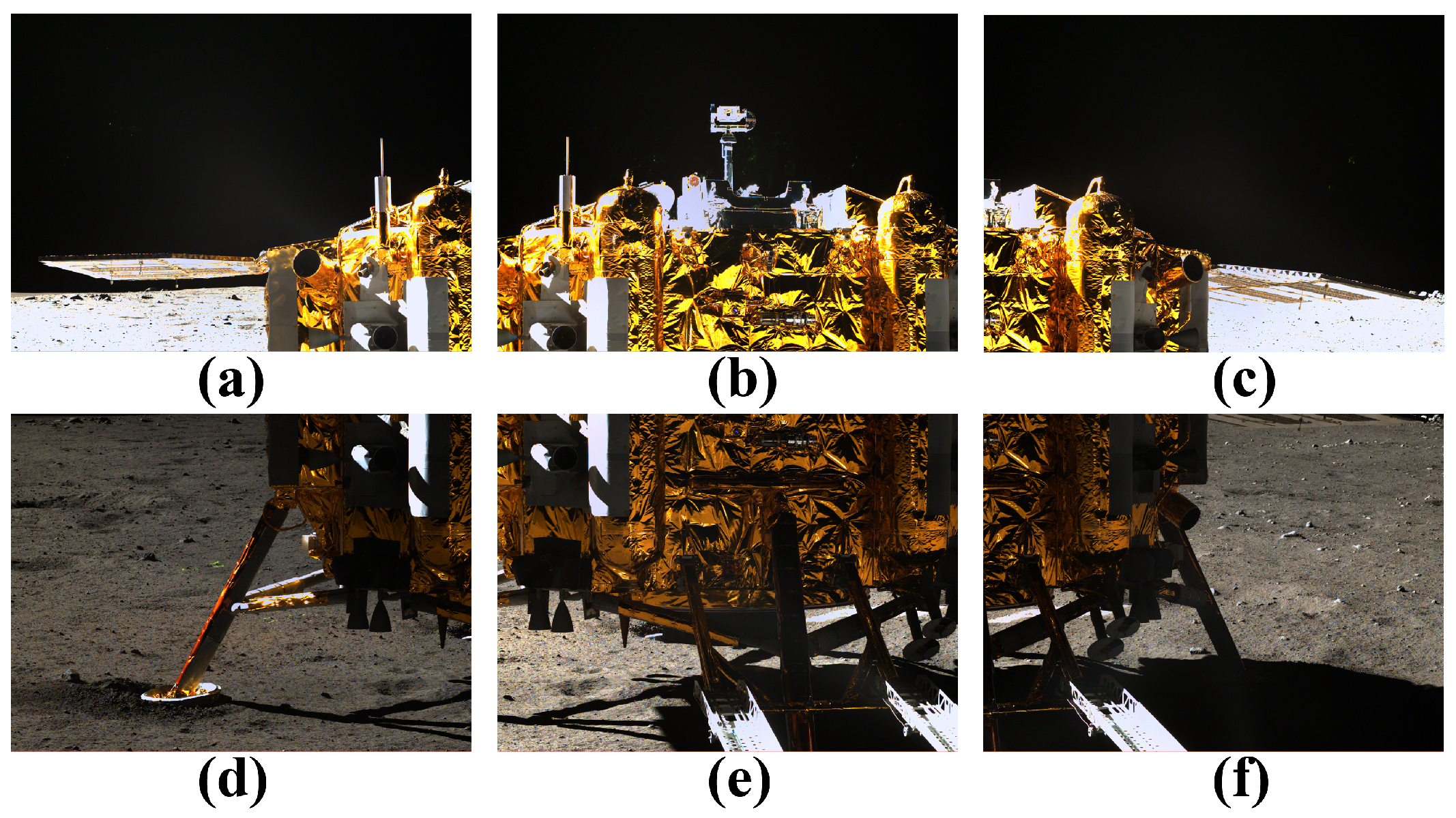
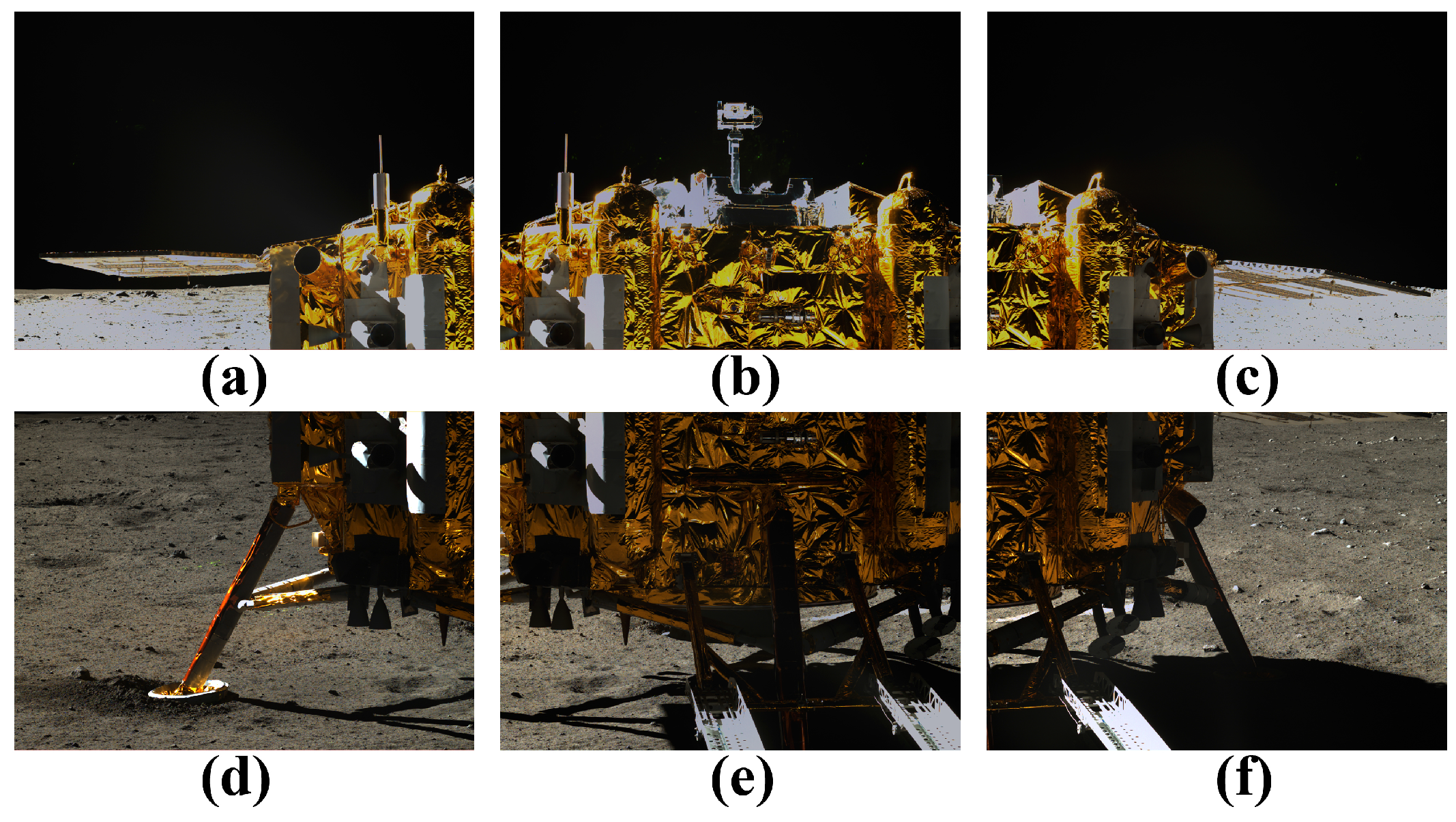
3.2. Experiments for Fusion

Fusion experiments were carried out on two adjacent images from the CE-3 PCAM. Again, the images were prepared by the geometric correction and pre-processing, and the mosaic images are shown in Figure 6. Selecting a cross section row of the mosaic image, the gray value of the overlapping region and adjacent images is displayed in Figure 7. From Figure 7, although the gray value of the left and right images are different, the fusion algorithm produced the smooth transition of the overlapping area and adjacent area.

4. Results and Discussion

Figure 8 demonstrates six color images of the lander, captured by the Yutu rover on 15 December 2013. At that time, the Yutu rover was located at the approximate due northerly direction, about 10 m from the lander. The site is named Point A, also named N0102(2, A), indicated in Figure 1. The CE-3 PCAM was set to the automatic exposure mode, and the overall brightness of these images is different because of the difference in the background. Figure 9 shows these images after the geometric correction and pre-processing. These images displayed in Figure 9 have higher contrast, lower noise, more consistent brightness range of values, and better visual effects.

Figure 10 is the lander panoramic mosaics that employed rectilinear projection (the projection of the panoramic sphere onto a flat surface, which is the projection that human eyes are most accustomed to) obtained from Figure 9 using the method described in Section 2. It is observed that this method solves the problems of the uneven illumination of CE-3 PCAM images and deals with the unique characteristics of the lunar surface image effectively. The PSNR and MSE between Figure 9 and Figure 10 are shown in

Table 4. $MSE$ (Mean Square Error) and $PSNR$ (Peak Signal to Noise Ratio) results of Red-Green-Blue channel in experiments shown in Figure 10.

Original Image	Adjacen Image	R-Channel		G-Channel		B-Channel
		$\mathit{MSE}$	$\mathit{PSNR}$ (dB)	$\mathit{MSE}$	$\mathit{PSNR}$ (dB)	$\mathit{MSE}$	$\mathit{PSNR}$ (dB)
a	b	14.6489	36.4727	13.5485	36.8119	8.3933	38.8915
b	c	18.2242	35.5243	18.6207	35.4308	8.0644	39.0651
d	e	42.3670	31.8605	38.7301	32.2503	29.6969	33.4037
e	f	32.7143	32.9834	26.7355	33.8599	12.0344	37.3266
d	a	5.9929	40.3545	4.7573	41.3572	2.5790	44.0163
e	b	30.8825	33.2337	26.3656	33.9204	4.0549	42.0510
f	c	4.5585	41.5425	3.8591	42.2660	1.8369	45.4899

.

The greater the $PSNR$ value, the higher the image fidelity, the better the quality. The quality was above average when the values of $PSNR$ in the range of 20∼30 dB, and the quality is better when the value is greater than 30 dB. As seen from Table 4, the $PSNR$ of the results in Figure 9 and Figure 10 are all between the values of 31 dB and 46 dB. The results of this study have indicated that the panoramic mosaicking method proposed in this paper has higher accuracy with a number of potential applications.

5. Conclusions

In this paper, we presented a unique approach to achieve the panoramic mosaics from CE-3 PCAM images. The key contributions of the study can be summarized in three aspects: (1) a novel image matching strategy is utilized to ensure that there is a sufficient number of correct matches under the condition of the lunar surface images. The effects of changes in external illumination can be handled well; (2) from an engineering point of view, the method we proposed in this study can achieve a mosaic in an effective way, i.e., can provide imagery of the lunar surface for surveying the terrain, geological features and structures, as well as prove useful for other scientific purposes; and (3) in the course of selecting the detected target and planning a path for the Yutu rover, the mosaic process played an important role in obtaining the correct orientation information. The engineering practices used in the CE-3 lunar mission have demonstrated that the mosaics obtained using the method proposed here were successfully applied for the mission plans. This method has been applied to all CE-3 PCAM images from the Point A site to produce a comprehensive view of the lunar surface at Point A.

References

1. Ip, W.H.; Yan, J.; Li, C.L.; Ouyang, Z.Y. Preface: The Chang’E-3 lander and rover mission to the Moon. Res. Astron. Astrophys. 2014, 14, 1511–1513. [Google Scholar] [CrossRef]
2. Bell III, J.F.; Squyres, S.W.; Arvidson, R.E.; Arneson, H.M.; Bass, D.; Blaney, D.; Cabrol, N.; Calvin, W.; Farmer, J.; Farrand, W.H.; et al. Pancam multispectral imaging results from the Spirit rover at Gusev crater. Science 2004, 305, 800–806. [Google Scholar] [CrossRef] [PubMed]
3. Bell, J.F., III; Squyres, S.W.; Arvidson, R.E.; Arneson, H.M.; Bass, D.; Calvin, W.; Farrand, W.H.; Goetz, W.; Golombek, M.; Greeley, R.; et al. Pancam multispectral imaging results from the Opportunity rover at Meridiani planum. Science 2004, 306, 1703–1709. [Google Scholar] [CrossRef] [PubMed]
4. Blake, D.F.; Morris, R.V.; Kocurek, G.; Morrison, S.M.; Downs, R.T.; Bish, D.; Ming, D.W.; Edgett, K.S.; Rubin, D.; Goetz, W.; et al. Curiosity at Gale crater, Mars: Characterization and analysis of the Rocknest sand shadow. Science 2013, 341. [Google Scholar] [CrossRef] [PubMed]
5. Grotzinger, J.P.; Sumner, D.Y.; Kah, L.C.; Stack, K.; Gupta, S.; Edgar, L.; Rubin, D.; Lewis, K.; Schieber, J.; Mangold, N.; et al. A habitable fluvio-lacustrine environment at Yellowknife bay, Gale crater, Mars. Science 2014, 343. [Google Scholar] [CrossRef] [PubMed]
6. Shum, H.Y.; Ng, K.T.; Chan, S.C. A virtual reality system using the concentric mosaic: Construction, rendering, and data compression. IEEE Trans. Multimed. 2005, 7, 85–95. [Google Scholar] [CrossRef] [Green Version]
7. Ngo, C.W.; Pong, T.C.; Zhang, H.J. Motion analysis and segmentation through spatio-temporal slices processing. IEEE Trans. Image Process. 2003, 12, 341–355. [Google Scholar] [PubMed]
8. Ma, Y.; Wang, L.; Zomaya, A.Y.; Chen, D.; Ranjan, R. Task-tree based large-scale mosaicking for massive remote sensed imageries with dynamic DAG scheduling. IEEE Trans. Parallel Distrib. Syst. 2014, 25, 2126–2137. [Google Scholar] [CrossRef]
9. Chen, C.; Chen, Z.; Li, M.; Liu, Y.; Cheng, L.; Ren, Y. Parallel relative radiometric normalisation for remote sensing image mosaics. Comput. Geosci. 2014, 73, 28–36. [Google Scholar] [CrossRef]
10. Bradley, P.; Jutzi, B. Improved feature detection in fused intensity-range images with complex SIFT (CSIFT). Remote Sens. 2011, 3, 2076–2088. [Google Scholar] [CrossRef]
11. Sima, A.; Buckley, S. Optimizing SIFT for matching of short wave infrared and visible wavelength images. Remote Sens. 2013, 5, 2073–2056. [Google Scholar] [CrossRef]
12. Chen, Q.; Wang, S.; Wang, B.; Sun, M. Automatic registration method for fusion of ZY-1-02C satellite images. Remote Sens. 2013, 5, 157–179. [Google Scholar] [CrossRef]
13. Wang, X.; Li, Y.; Wei, H.; Liu, F. An ASIFT-based local registration method for satellite imagery. Remote Sens. 2015, 7, 7044–7061. [Google Scholar] [CrossRef]
14. Brown, L.G. A survey of image registration techniques. ACM Comput. Surv. 1992, 24, 325–376. [Google Scholar] [CrossRef]
15. Matas, J.; Chum, O.; Urban, M.; Pajdla, T. Robust wide-baseline stereo from maximally stable extremal regions. Image Vis. Comput. 2004, 22, 761–767. [Google Scholar] [CrossRef]
16. Canny, J. A computational approach to edge detection. IEEE Trans. Pattern Anal. Mach. Intell. 1986, 8, 679–698. [Google Scholar] [CrossRef] [PubMed]
17. Mokhtarian, F.; Suomela, R. Robust image corner detection through curvature scale space. IEEE Trans. Pattern Anal. Mach. Intell. 1998, 20, 1376–1381. [Google Scholar] [CrossRef]
18. Mikolajczyk, K.; Schmid, C. A performance evaluation of local descriptors. IEEE Trans. Pattern Anal. Mach. Intell. 2005, 27, 1615–1630. [Google Scholar] [CrossRef] [PubMed]
19. Wu, F.; Liu, J.; Ren, X.; Li, C. Deep space exploration panoramic camera calibration technique based on circular markers. Acta Opt. Sin. 2013, 33. [Google Scholar] [CrossRef]
20. Brown, D. Decentering distortion of lenses. Photom. Eng. 1966, 32, 444–462. [Google Scholar]
21. Brown, D. Close-range camera calibration. Photom. Eng. 1971, 37, 855–866. [Google Scholar]
22. Fryer, J.; Brown, D. Lens distortion for close-range photogrammetry. Photogramm. Eng. Remote Sens. 1986, 52, 51–58. [Google Scholar]
23. Tsai, R. A versatile camera calibration technique for high-accuracy 3D machine vision metrology using off-the-shelf TV cameras and lenses. IEEE J. Robot. Autom. 1987, 3, 323–344. [Google Scholar] [CrossRef]
24. Wang, W.R.; Ren, X.; Wang, F.F.; Liu, J.J.; Li, C.L. Terrain reconstruction from Chang’e-3 PCAM images. Res. Astron. Astrophys. 2015, 15, 1057–1067. [Google Scholar] [CrossRef]
25. More, J.J. The Levenberg–Marquardt algorithm: Implementation and theory. Numer. Anal. 1978, 630, 105–116. [Google Scholar]
26. Dunlap, J.C.; Bodegom, E.; Widenhorn, R. Correction of dark current in consumer cameras. J. Electron. Imaging 2010, 19. [Google Scholar] [CrossRef]
27. Dunlap, J.C.; Porter, W.C.; Bodegom, E.; Widenhorn, R. Dark current in an active pixel complementary metal-oxide-semiconductor sensor. J. Electron. Imaging 2011, 20. [Google Scholar] [CrossRef]
28. Ren, X.; Li, C.; Liu, J.; Wang, F.; Yang, J.; Liu, E.; Xue, B.; Zhao, R. A method and results of color calibration for the Chang’e-3 terrain camera and panoramic camera. Res. Astron. Astrophys. 2014, 14, 1557–1566. [Google Scholar] [CrossRef]
29. Moravec, H. Towards automatic visual obstacle avoidance. In Proceedings of the 5th International Joint Conference on Artificial Intelligence, Cambridge, MA, USA, 22–25 August 1977; p. 584.
30. Harris, C.; Stephens, M. A combined corner and edge detector. In Proceedings of the Alvey Vision Conference, Manchester, UK, 31 August–2 September 1988; pp. 147–151.
31. Smith, S.; Brady, J. SUSAN—A new approach to low level image processing. Int. J. Comput. Vis. 1997, 23, 45–78. [Google Scholar] [CrossRef]
32. Mukherjee, D.; Wu, Q.; Wang, G. A comparative experimental study of image feature detectors and descriptors. Mach. Vis. Appl. 2015, 26, 443–466. [Google Scholar] [CrossRef]
33. Lowe, D.G. Distinctive image features from scale-invariant keypoints. Int. J. Comput. Vis. 2004, 60, 91–110. [Google Scholar] [CrossRef]
34. Brown, M.; Lowe, D.G. Automatic panoramic image stitching using invariant features. Int. J. Comput. Vis. 2007, 74, 59–73. [Google Scholar] [CrossRef]
35. Bay, H.; Ess, A.; Tuytelaars, T.; Van Gool, L. Speeded-up robust features (SURF). Comput. Vis. Image Underst. 2008, 110, 346–359. [Google Scholar] [CrossRef]
36. Fischler, M.A.; Bolles, R.C. Random sample consensus: A paradigm for model fitting with applications to image analysis and automated cartography. Commun. ACM 1981, 24, 381–395. [Google Scholar] [CrossRef]
Figure 1. The Yutu Rover route sketch. PCAM (Panoramic Camera) working at “exploration”, navigation camera working at “navigation”. The red dotted line means planned future route.
Remotesensing 08 00812 g001
Figure 2. Main steps of the proposed method.
Remotesensing 08 00812 g002
Figure 3. Diagram showing the panoramic capture process for a single camera, where I k ( k = 1 , 2 , . . . , 6 ) = image, I p = combined panorama, and O = optical center of the camera.
Remotesensing 08 00812 g003
Figure 4. Sample images from the CE-3 PCAM (Panoramic Camera). (a,b) are adjacent images under sidelight; (c,d) are adjacent images under frontlighting.
Remotesensing 08 00812 g004
Figure 5. Schematic of feature matching when t h r = 0.4. (a) a,b using SIFT (Scale Invariant Feature Transform) algorithm; (b) a,b using SURF (Speed-Up Robust Features)algorithm.
Remotesensing 08 00812 g005
Figure 6. Original images and mosaic image. (a) left original image; (b) right original image; (c) mosaic image.
Remotesensing 08 00812 g006
Figure 7. Schematic of gray value. The horizontal axis is the X-coordinate of pixel. The vertical axis represents the corresponding gray value.
Remotesensing 08 00812 g007
Figure 8. Original images recorded at Point A. (a) upper-left image; (b) upper-middle image; (c) upper-right image; (d) lower-left image; (e) lower-middle image; (f) lower-right image.
Remotesensing 08 00812 g008
Figure 9. Images after the geometric correction and pre-processing. (a) upper-left image; (b) upper-middle image; (c) upper-right image; (d) lower-left image; (e) lower-middle image; (f) lower-right image.
Remotesensing 08 00812 g009
Figure 10. Lander panoramic mosaic image.
Remotesensing 08 00812 g010