
Incorporating Diversity into Self-Learning for Synergetic Classification of Hyperspectral and Panchromatic Images


Abstract
:
1. Introduction
2. Materials and Methodology
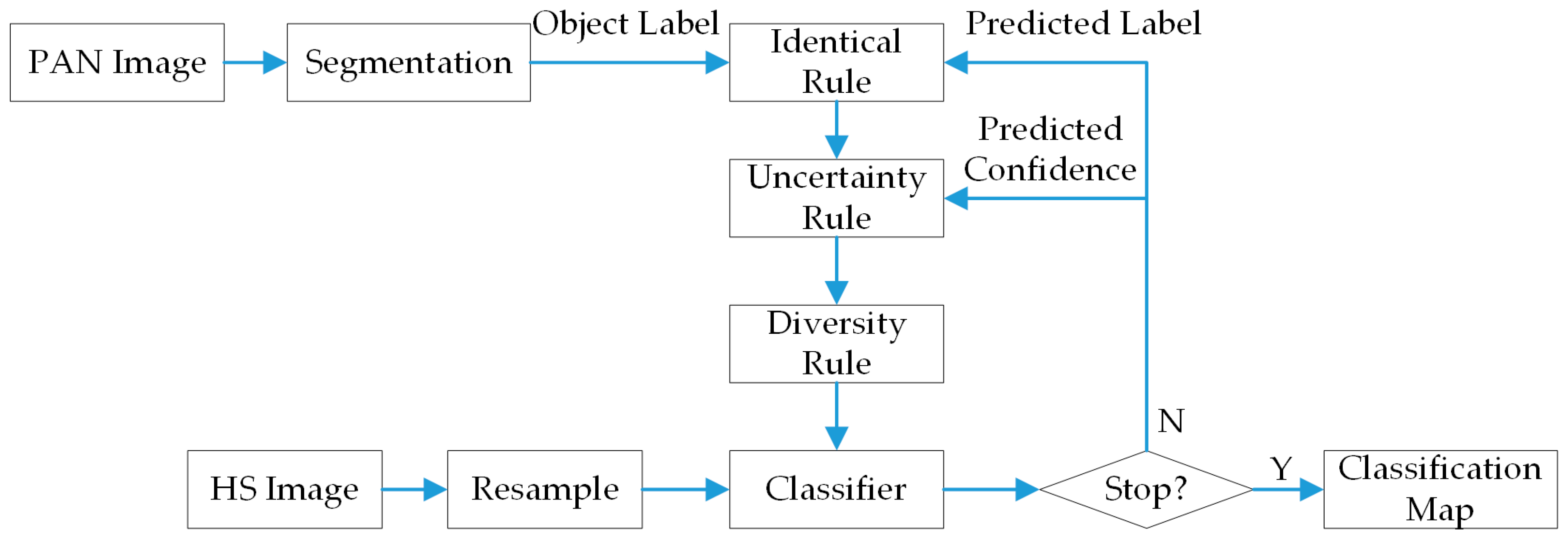
2.1. Data Sets
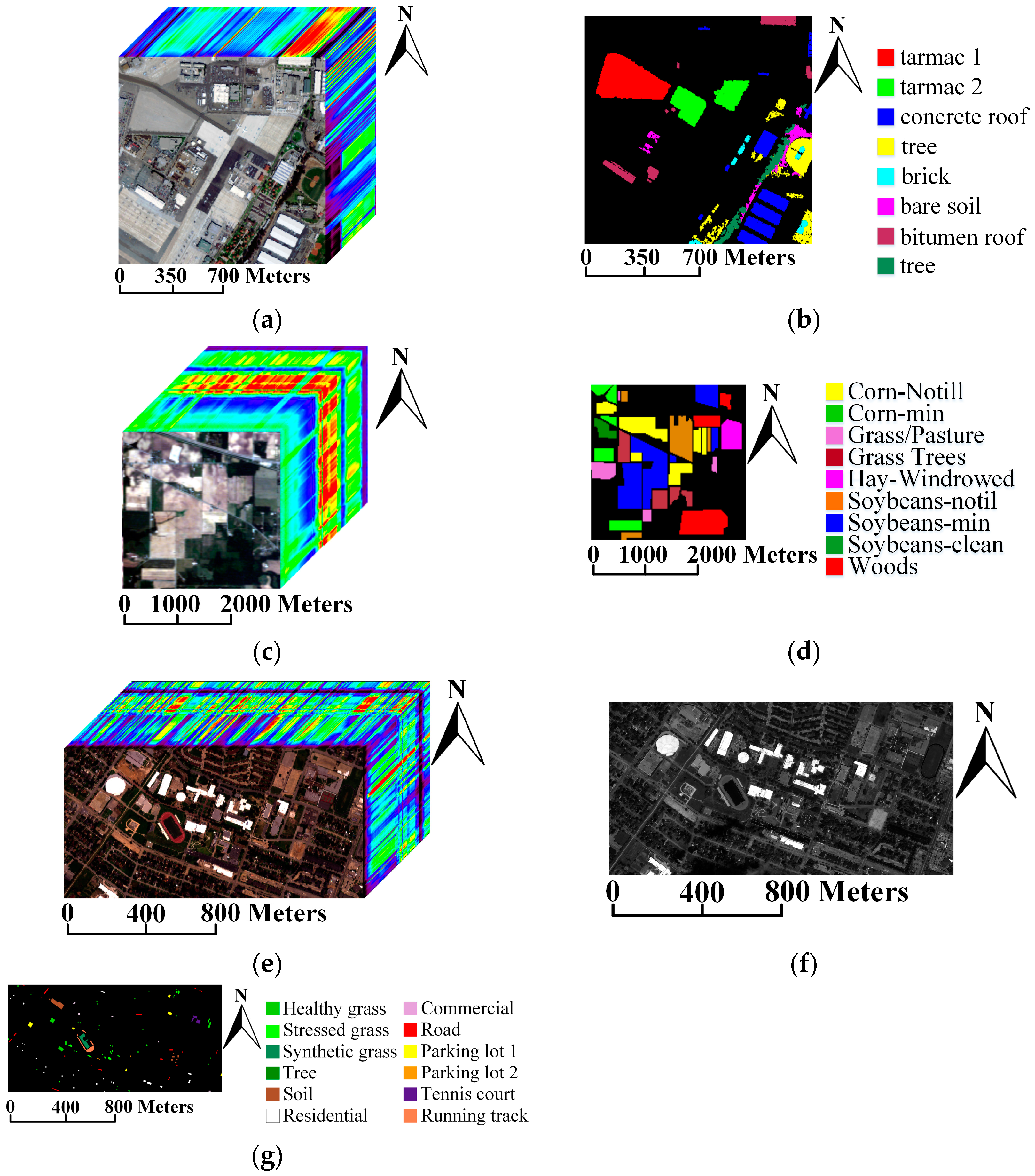
2.2. Related Work
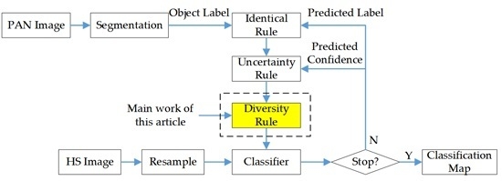
2.3. Implementation of Diversity Criteria within SL
| Algorithm 1. AL combined with similarity measure–based diversity criterion |
| Input: Candidate set , number of classes , number of selected samples ; |
| Output: Totally samples included in ; |
| 1. Select most informative samples via AL strategy, denoted as ; |
| For = 1 to |
| 2. Select the samples of class from , denoted as ; |
| 3. ; |
| 4. If the number of samples in is less than , then put them into , |
| Otherwise: |
| 5. Pick out the most uncertain sample from , and put it into ; |
| 6. For each sample , compute the mean value of distance (negative value of spatial distance or the KCA value) with the samples in ; |
| 7. Pick out the sample that has minimum mean value, and put it into ; |
| 8. Repeat steps 6 and 7 until has samples; |
| End for |
| Algorithm 2. AL combined with cluster-based diversity criterion |
| Input: Candidate set , number of classes , number of selected samples ; |
| Output: Total samples included in ; |
| 1. Select most informative samples via AL strategy, denoted as ; |
| For = 1 to |
| 2. Select the samples of the class from , denoted as ; |
| 3. ; |
| 4. If the number of samples in is less than , then put them into , |
| Otherwise: |
| 5. Apply kernel k-means clustering to , the cluster number is ; |
| 6. Select the most uncertain sample of each cluster, and put it into , until has samples; |
| End for |
3. Experimental Results and Analyses
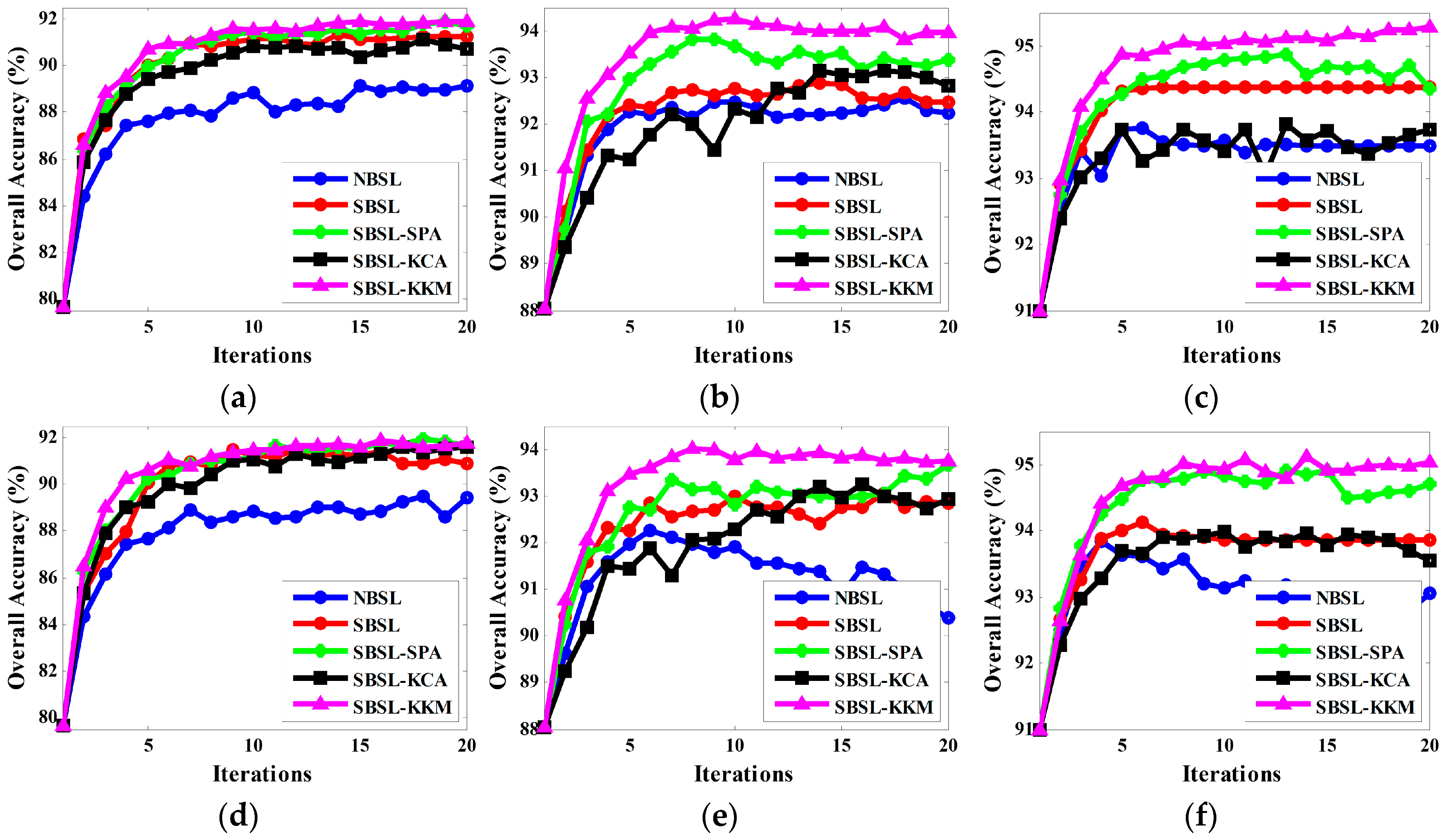
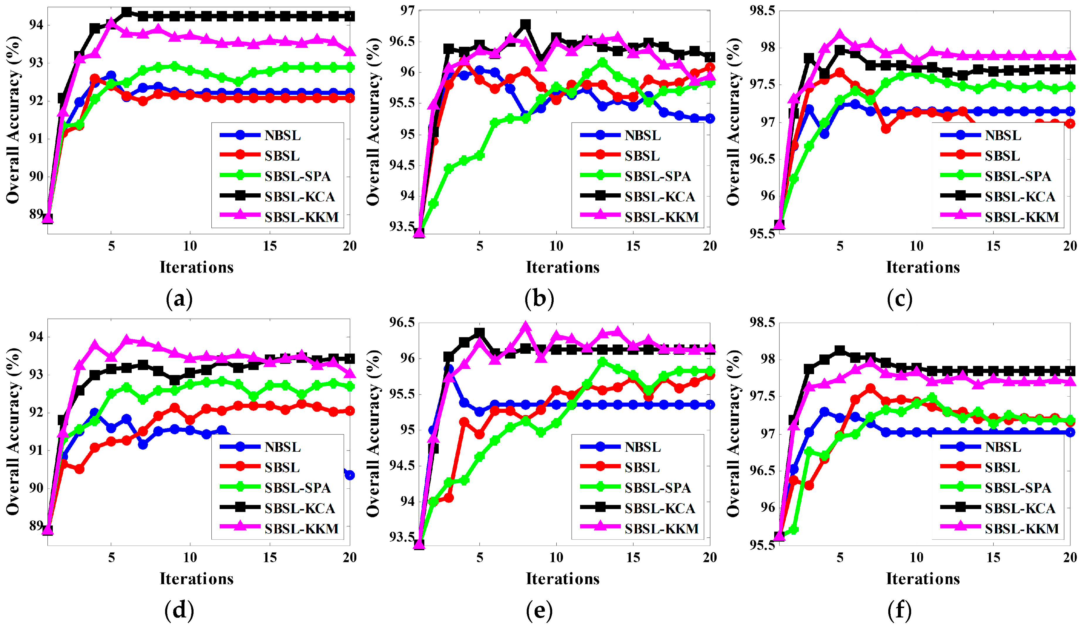
3.1. Experimental Results on Simulated Data Set
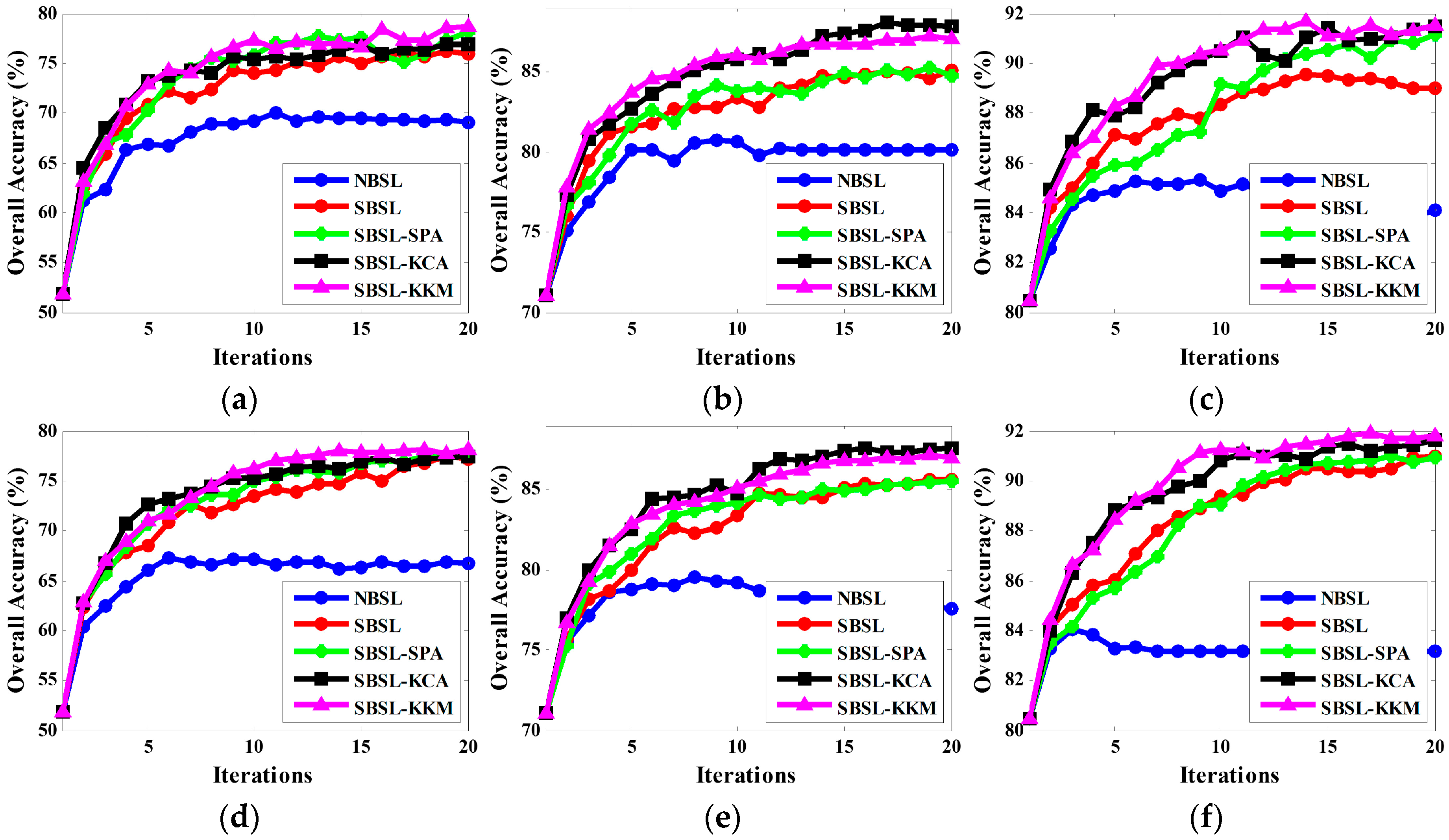
3.2. Experimental Results on Real Data Set
4. Discussion
5. Conclusions
Supplementary Materials
Acknowledgments
Author Contributions
Conflicts of Interest
References
- Lu, D.; Weng, Q. A survey of image classification methods and techniques for improving classification performance. Int. J. Remote Sens. 2007, 28, 823–870. [Google Scholar] [CrossRef]
- Ballanti, L.; Blesius, L.; Hines, E.; Kruse, B. Tree species classification using hyperspectral imagery: A comparison of two classifiers. Remote Sens. 2016, 8, 445. [Google Scholar] [CrossRef]
- Sami ul Haq, Q.; Tao, L.; Sun, F.; Yang, S. A fast and robust sparse approach for hyperspectral data classification using a few labeled samples. IEEE Trans. Geosci. Remote Sens. 2012, 50, 2287–2302. [Google Scholar] [CrossRef]
- Wang, Z.; Du, B.; Zhang, L.; Zhang, L. A batch-mode active learning framework by querying discriminative and representative samples for HS image classification. Neurocomputing 2016, 179, 88–100. [Google Scholar] [CrossRef]
- Patra, S.; Bruzzone, L. A fast cluster-assumption based active-learning technique for classification of remote sensing images. IEEE Trans. Geosci. Remote Sens. 2011, 49, 1617–1626. [Google Scholar] [CrossRef]
- Persello, C.; Bruzzone, L. Active and semisupervised learning for the classification of remote sensing images. IEEE Trans. Geosci. Remote Sens. 2014, 52, 6937–6956. [Google Scholar] [CrossRef]
- Marconcini, M.; Camps-Valls, G.; Bruzzone, L. A composite semisupervised SVM for classification of hyperspectral images. IEEE Geosci. Remote Sens. Lett. 2009, 6, 234–238. [Google Scholar] [CrossRef]
- Mingmin, C.; Bruzzone, L. Semisupervised classification of hyperspectral images by SVMs optimized in the primal. IEEE Trans. Geosci. Remote Sens. 2007, 45, 1870–1880. [Google Scholar]
- Mitchell, T. The role of unlabeled data in supervised learning. In Proceedings of the Sixth International Colloquium on Cognitive Science, San Sebastian, Spain, 12–19 May 1999; pp. 1–8.
- Fujino, A.; Ueda, N.; Saito, K. A hybrid generative/ discriminative approach to semi-supervised classifier design. In Proceedings of the 20th National Conference on Artificial Intelligence, Pittsburgh, PA, USA, 9–13 July 2005; pp. 764–769.
- Bruzzone, L.; Chi, M.; Marconcini, M. A novel transductive SVM for semi-supervised classification of remote-sensing images. IEEE Trans. Geosci. Remote Sens. 2006, 44, 3363–3373. [Google Scholar] [CrossRef]
- Camps-Valls, G.; Bandos Marsheva, T.; Zhou, D. Semi-supervised graph-based hyperspectral image classification. IEEE Trans. Geosci. Remote Sens. 2007, 45, 3044–3054. [Google Scholar] [CrossRef]
- Zhu, X. Semi-supervised learning literature survey. Comput. Sci. 2008, 37, 63–77. [Google Scholar]
- Zhang, L.; Chen, C.; Bu, J.; Cai, D.; He, X.; Huang, T.S. Active learning based on locally linear reconstruction. IEEE Trans. Pattern Anal. Mach. Intell. 2011, 33, 2026–2038. [Google Scholar] [CrossRef] [PubMed]
- Zomer, S.; Sànchez, M.N.; Brereton, R.G.; Pérez-Pavón, J.L. Active learning support vector machines for optimal sample selection in classification. J. Chemom. 2004, 18, 294–305. [Google Scholar] [CrossRef]
- Campbell, C.; Cristianini, N.; Smola, A.J. Query learning with large margin classifiers. In Proceedings of the 17th International Conference on Machine Learning, Stanford, CA, USA, June 29–2 July 2000; pp. 111–118.
- Tuia, D.; Pasolli, E.; Emery, W.J. Using active learning to adapt remote sensing image classifiers. Remote Sens. Environ. 2011, 115, 2232–2242. [Google Scholar] [CrossRef]
- Tuia, D.; Volpi, M.; Copa, L.; Kanevski, M.; Munoz-Mari, J. A survey of active learning algorithms for supervised remote sensing image classification. IEEE J. Sel. Top. Signal Process. 2011, 5, 606–617. [Google Scholar] [CrossRef]
- Xia, G.; Wang, Z.; Xiong, C.; Zhang, L. Accurate annotation of remote sensing images via active spectral clustering with little expert knowledge. Remote Sens. 2015, 7, 15014–15045. [Google Scholar] [CrossRef]
- Dopido, I.; Li, J.; Marpu, P.R.; Plaza, A.; Dias, J.M.B.; Benediktsson, J.A. Semisupervised self-learning for hyperspectral image classification. IEEE Trans. Geosci. Remote Sens. 2013, 51, 4032–4044. [Google Scholar] [CrossRef]
- Lu, X.; Zhang, J.; Li, T.; Zhang, Y. A novel synergetic classification approach for hyperspectral and panchromatic images based on self-learning. IEEE Trans. Geosci. Remote Sens. 2016, 54, 4917–4928. [Google Scholar] [CrossRef]
- Brinker, K. Incorporating diversity in active learning with support vector machines. In Proceedings of the 20th International Conference on Machine Learning, Washington, DC, USA, 21–24 August 2003; pp. 59–66.
- Nguyen, H.T.; Smeulders, A. Active learning using pre-clustering. In Proceedings of the 21th International Conference on Machine Learning, Banff, AB, Canada, 4–8 July 2004; pp. 623–630.
- Stavrakoudis, D.G.; Dragozi, E.; Gitas, I.Z.; Karydas, C.G. Decision fusion based on hyperspectral and multispectral satellite imagery for accurate forest species mapping. Remote Sens. 2014, 6, 6897–6928. [Google Scholar] [CrossRef]
- Bouziani, M.; Goita, K.; He, D. Rule-based classification of a very high resolution image in an urban environment using multispectral segmentation guided by Cartographic data. IEEE Trans. Geosci. Remote Sens. 2010, 48, 3198–3211. [Google Scholar] [CrossRef]
- Ghamisi, P.; Couceiro, M.S.; Fauvel, M.; Benediktsson, J.A. Integration of segmentation techniques for classification of hyperspectral images. IEEE Geosci. Remote Sens. Lett. 2014, 11, 342–346. [Google Scholar] [CrossRef]
- Wang, M.; Li, R. Segmentation of high spatial resolution remote sensing imagery based on hard-boundary constraint and two-stage merging. IEEE Trans. Geosci. Remote Sens. 2014, 52, 5712–5725. [Google Scholar] [CrossRef]
- Crisp, D. Improved data structures for fast region merging segmentation using A Mumford-Shah energy functional. In Proceedings of Digital Image Computing: Techniques and Applications (DICTA), Canberra, Australia, 1–3 December 2008; pp. 586–592.
- Demir, B.; Persello, C.; Bruzzone, L. Batch-mode active-learning methods for the interactive classification of Remote Sensing Image. IEEE Trans. Geosci. Remote Sens. 2011, 49, 1014–1031. [Google Scholar] [CrossRef]
- Tuia, D.; Ratle, F.; Pacifici, F.; Kanevski, M.; Emery, W.J. Active learning methods for remote sensing image classification. IEEE Trans. Geosci. Remote Sens. 2009, 47, 2218–2232. [Google Scholar] [CrossRef]
- Xu, Z.; Yu, K.; Tresp, V.; Xu, X.; Wang, J. Representative sampling for text classification using support vector machines. In Proceedings of the 25th European Conference on Information Retrieval, Pisa, Italy, 14–16 April 2003; pp. 393–407.
- Pasolli, E.; Melgani, F.; Tuia, D.; Pacifici, F.; Emery, W.J. SVM active learning approach for image classification using spatial information. IEEE Trans. Geosci. Remote Sens. 2014, 52, 2217–2233. [Google Scholar] [CrossRef]
- Stumpf, A.; Lachiche, N.; Malet, J.; Kerle, N.; Puissant, A. Active learning in the spatial domain for remote sensing image classification. IEEE Trans. Geosci. Remote Sens. 2014, 52, 2492–2507. [Google Scholar] [CrossRef]
- Demir, B.; Minello, L.; Bruzzone, L. Definition of effective training sets for supervised classification of remote sensing images by a novel cost-sensitive active learning method. IEEE Trans. Geosci. Remote Sens. 2014, 52, 1271–1284. [Google Scholar] [CrossRef]
- Girolami, M. Mercer kernel-based clustering in feature space. IEEE Trans. Neural Netw. 2002, 13, 780–784. [Google Scholar] [CrossRef] [PubMed]
- Zhang, R.; Rudnicky, A.I. A large scale clustering scheme for kernel K-Means. In Proceedings of the 16th International Conference on Pattern Recognition, Quebec City, QC, Canada, 11–15 August 2002; pp. 289–292.
- Melgani, F.; Bruzzone, L. Classification of hyperspectral remote sensing images with support vector machines. IEEE Trans. Geosci. Remote Sens. 2004, 42, 1778–1790. [Google Scholar] [CrossRef]
- Yu, H.; Gao, L.; Li, J.; Li, S.S.; Zang, B.; Benediktsson, J.A. Spectral-spatial hyperspectral image classification using subspace-based support vector machines and adaptive Markov random fields. Remote Sens. 2016, 8, 355. [Google Scholar] [CrossRef]
- Wohlberg, B.; Tartakovsky, D.M.; Guadagnini, A. Subsurface characterization with support vector machines. IEEE Trans. Geosci. Remote Sens. 2006, 44, 47–57. [Google Scholar] [CrossRef]
- Mathur, A.; Foody, G.M. Multiclass and binary SVM classification: Implications for training and classification users. IEEE Geosci. Remote Sens. Lett. 2008, 5, 241–245. [Google Scholar] [CrossRef]
- Mountrakis, G.; Im, J.; Ogole, C. Support vector machines in remote sensing: A review. ISPRS J. Photogramm. Remote Sens. 2011, 66, 247–259. [Google Scholar] [CrossRef]
- Kwok, J.T.-Y. Moderating the outputs of support vector machine classifiers. IEEE Trans. Neural Netw. 1999, 10, 1018–1031. [Google Scholar] [CrossRef] [PubMed]


| San Diego | 5 Labeled Samples per Class, 40 Unlabeled Samples per Iteration | |||||||||||
| SVM | NBSL | SBSL | SBSL-SPA | SBSL-KCA | SBSL-KKM | |||||||
| MBT | MMS | MBT | MMS | MBT | MMS | MBT | MMS | MBT | MMS | |||
| OA | 79.64 ± 4.59 | 89.13 ± 2.97 | 89.44 ± 2.59 | 91.24 ± 2.91 | 90.89 ± 2.06 | 91.72 ± 2.34 | 91.68 ± 2.60 | 90.74 ± 2.32 | 91.57 ± 2.23 | 91.89 ± 2.38 | 91.78 ± 2.95 | |
| Kappa | 0.7591 ± 0.0528 | 0.8708 ± 0.0349 | 0.8743 ± 0.0305 | 0.8956 ± 0.0343 | 0.8914 ± 0.0244 | 0.9010 ± 0.0279 | 0.9006 ± 0.0310 | 0.8897 ± 0.0274 | 0.8995 ± 0.0263 | 0.9032 ± 0.0284 | 0.9019 ± 0.0351 | |
| 10 labeled samples per class, 64 unlabeled samples per iteration | ||||||||||||
| SVM | NBSL | SBSL | SBSL-SPA | SBSL-KCA | SBSL-KKM | |||||||
| MBT | MMS | MBT | MMS | MBT | MMS | MBT | MMS | MBT | MMS | |||
| OA | 88.03 ± 1.70 | 92.24 ± 1.89 | 90.39 ± 2.02 | 92.47 ± 1.93 | 92.86 ± 2.73 | 93.36 ± 1.88 | 93.66 ± 2.03 | 92.81 ± 1.60 | 92.92 ± 2.70 | 93.95 ± 1.85 | 93.76 ± 2.24 | |
| Kappa | 0.8575 ± 0.0202 | 0.9076 ± 0.0224 | 0.8850 ± 0.0240 | 0.9105 ± 0.0228 | 0.9150 ± 0.0322 | 0.9208 ± 0.0223 | 0.9243 ± 0.0240 | 0.9144 ± 0.0189 | 0.9158 ± 0.0318 | 0.9278 ± 0.0218 | 0.9256 ± 0.0265 | |
| 15 labeled samples per class, 80 unlabeled samples per iteration | ||||||||||||
| SVM | NBSL | SBSL | SBSL-SPA | SBSL-KCA | SBSL-KKM | |||||||
| MBT | MMS | MBT | MMS | MBT | MMS | MBT | MMS | MBT | MMS | |||
| OA | 91.00 ± 1.70 | 93.48 ± 1.01 | 93.05 ± 1.60 | 94.38 ± 1.58 | 93.85 ± 2.45 | 94.35 ± 0.41 | 94.71 ± 0.97 | 93.73 ± 1.69 | 93.54 ± 1.16 | 95.29 ± 0.41 | 95.03 ± 0.83 | |
| Kappa | 0.8927 ± 0.0200 | 0.9222 ± 0.0119 | 0.9172 ± 0.0189 | 0.9328 ± 0.0186 | 0.9265 ± 0.0287 | 0.9325 ± 0.0049 | 0.9369 ± 0.0115 | 0.9253 ± 0.0201 | 0.9230 ± 0.0137 | 0.9437 ± 0.0050 | 0.9406 ± 0.0099 | |
| Indian Pines | 5 labeled samples per class, 27 unlabeled samples per iteration | |||||||||||
| SVM | NBSL | SBSL | SBSL-SPA | SBSL-KCA | SBSL-KKM | |||||||
| MBT | MMS | MBT | MMS | MBT | MMS | MBT | MMS | MBT | MMS | |||
| OA | 51.85 ± 8.92 | 69.07 ± 5.39 | 66.78 ± 3.69 | 75.90 ± 4.71 | 77.14 ± 3.86 | 78.12 ± 4.57 | 77.47 ± 4.29 | 76.84 ± 5.08 | 77.46 ± 6.41 | 78.64 ± 4.72 | 78.17 ± 6.10 | |
| Kappa | 0.4454 ± 0.0974 | 0.6410 ± 0.0604 | 0.6146 ± 0.0.415 | 0.7190 ± 0.0531 | 0.7322 ± 0.0445 | 0.7432 ± 0.0531 | 0.7361 ± 0.0494 | 0.7284 ± 0.0578 | 0.7359 ± 0.0733 | 0.7497 ± 0.0549 | 0.7446 ± 0.0697 | |
| 10 labeled samples per class, 36 unlabeled samples per iteration | ||||||||||||
| SVM | NBSL | SBSL | SBSL-SPA | SBSL-KCA | SBSL-KKM | |||||||
| MBT | MMS | MBT | MMS | MBT | MMS | MBT | MMS | MBT | MMS | |||
| OA | 71.05 ± 4.42 | 80.17 ± 3.52 | 77.56 ± 2.89 | 85.07 ± 4.06 | 85.60 ± 3.22 | 84.75 ± 3.17 | 85.51 ± 3.08 | 87.83 ± 2.36 | 87.58 ± 2.41 | 87.09 ± 1.81 | 87.00 ± 3.02 | |
| Kappa | 0.6644 ± 0.0457 | 0.7685 ± 0.0399 | 0.7387 ± 0.0325 | 0.8251 ± 0.0467 | 0.8311 ± 0.0370 | 0.8211 ± 0.0362 | 0.8301 ± 0.0353 | 0.8568 ± 0.0274 | 0.8538 ± 0.0280 | 0.8483 ± 0.0206 | 0.8473 ± 0.0348 | |
| 15 labeled samples per class, 45 unlabeled samples per iteration | ||||||||||||
| SVM | NBSL | SBSL | SBSL-SPA | SBSL-KCA | SBSL-KKM | |||||||
| MBT | MMS | MBT | MMS | MBT | MMS | MBT | MMS | MBT | MMS | |||
| OA | 80.49 ± 2.80 | 84.09 ± 3.04 | 83.14 ± 3.24 | 89.00 ± 4.54 | 90.97 ± 1.90 | 91.15 ± 1.77 | 90.92 ± 1.54 | 91.45 ± 2.32 | 91.65 ± 2.40 | 91.53 ± 1.77 | 91.80 ± 1.73 | |
| Kappa | 0.77150.0324 | 0.8132 ± 0.0353 | 0.8019 ± 0.0205 | 0.8705 ± 0.0525 | 0.8933 ± 0.0223 | 0.8954 ± 0.0208 | 0.8924 ± 0.0181 | 0.8987 ± 0.0271 | 0.9011 ± 0.0281 | 0.9015 ± 0.0209 | 0.9028 ± 0.0205 | |
© 2016 by the authors; licensee MDPI, Basel, Switzerland. This article is an open access article distributed under the terms and conditions of the Creative Commons Attribution (CC-BY) license (http://creativecommons.org/licenses/by/4.0/).
Share and Cite
Lu, X.; Zhang, J.; Li, T.; Zhang, Y. Incorporating Diversity into Self-Learning for Synergetic Classification of Hyperspectral and Panchromatic Images. Remote Sens. 2016, 8, 804. https://doi.org/10.3390/rs8100804
Lu X, Zhang J, Li T, Zhang Y. Incorporating Diversity into Self-Learning for Synergetic Classification of Hyperspectral and Panchromatic Images. Remote Sensing. 2016; 8(10):804. https://doi.org/10.3390/rs8100804
Chicago/Turabian StyleLu, Xiaochen, Junping Zhang, Tong Li, and Ye Zhang. 2016. "Incorporating Diversity into Self-Learning for Synergetic Classification of Hyperspectral and Panchromatic Images" Remote Sensing 8, no. 10: 804. https://doi.org/10.3390/rs8100804