Short-Term Change Detection in Wetlands Using Sentinel-1 Time Series

Abstract

Automated monitoring systems that can capture wetlands’ high spatial and temporal variability are essential for their management. SAR-based change detection approaches offer a great opportunity to enhance our understanding of complex and dynamic ecosystems. We test a recently-developed time series change detection approach (S1-omnibus) using Sentinel-1 imagery of two wetlands with different ecological characteristics; a seasonal isolated wetland in southern Spain and a coastal wetland in the south of France. We test the S1-omnibus method against a commonly-used pairwise comparison of consecutive images to demonstrate its advantages. Additionally, we compare it with a pairwise change detection method using a subset of consecutive Landsat images for the same period of time. The results show how S1-omnibus is capable of capturing in space and time changes produced by water surface dynamics, as well as by agricultural practices, whether they are sudden changes, as well as gradual. S1-omnibus is capable of detecting a wider array of short-term changes than when using consecutive pairs of Sentinel-1 images. When compared to the Landsat-based change detection method, both show an overall good agreement, although certain landscape changes are detected only by either the Landsat-based or the S1-omnibus method. The S1-omnibus method shows a great potential for an automated monitoring of short time changes and accurate delineation of areas of high variability and of slow and gradual changes.

1. Introduction

Wetlands are often described as ecotones, transitional habitats situated between dry land (upland) and water bodies [1]. They are very diverse ecosystems, ranging from permanent water bodies to lands that remain completely dry over several months, or areas where water is below a dense vegetation cover, such as peat bogs or mangroves [2]. Besides their spatial variability, some wetlands present a high temporal variability (e.g., temporal water bodies and waterways or intertidal flats). Wetlands also deliver a wide and well-recognized array of ecosystem services: flooding, drought and erosion amelioration, habitat for many keystone species, food and water supply and CO₂ sequestration, among many others [3]. Thus, automated monitoring systems of wetlands that can capture their high temporal and spatial variability are essential for wetland management and for the quantification of the ecosystem services they provide [4].

Landscape spatial patterns, and especially those of wetlands, are rarely static due to intra-annual changes in their ecosystem properties, whether they are caused by natural or by anthropogenic factors [5]. Mapping of ecosystems and of long-term Land Use and Land Cover Change (LULCC) patterns may be biased by such intra-annual changes in different surface properties (e.g., phenology, hydrology, agriculture, etc.). These surface dynamics sometimes produce transitional states and fine-scale mixtures of classes that may hinder classification and long-term change detection. Some approaches have used fuzzy classifiers and multitemporal optical data to produce fractional cover maps of different wetland classes, capturing these transitional states [6]. Additionally, [7] proposed the term “Dynamic Cover Types” (DCT) to refer to areas of frequent periodic or seasonal change. Examples of DCT in the context of wetlands would be seasonally-inundated floodplains and inland valleys, inter-tidal flats, temporal water bodies and waterways, fields of rice and reeds when harvested or slow regrowth of some vegetation covers after flooding or harvesting events. Many of these DCT often give rise to unique species assemblages and temporal shifting of species distributions and compositions [8,9]. In turn, this may also affect other ecosystem functions through water and nutrient cycling.

The availability of satellite images acquired repetitively over long periods of time has allowed the proliferation of numerous change detection studies in fields, such as LULC change, forest monitoring (deforestation, regeneration, forest fires, insect defoliation), urban sprawl, landscape change and crop monitoring, among many others; [10] provides a wide array of examples of applications in each mentioned field. Most of these techniques make use of spectral data from optical sensors to monitor long-term changes. Despite their widely-spread use and the good results obtained, optical-based change detection methods have an important disadvantage; they are hampered by illumination effects and cloud conditions, a challenge that becomes very problematic in sub-humid to humid tropics, especially during rainy seasons or when the temporal resolution is not high. SAR-based change detection methods are cloud and illumination independent, but have however been much less used because of their limited temporal and spatial availability, higher costs and more intensive processing requirements [11]. With the recent launch of ESA’s Sentinel-1 satellite and the free access to its products, SAR-based change detection methods can now be more efficiently used to overcome some of the restrictions of optical-based methods. The high temporal resolution (six days considering Sentinel-1A and -1B at the Equator), high spatial resolution and wide swath allow for a much-needed operational change detection system, cost-free, cloud-proof and illumination independent.

SAR-based change detection methods can separate LULC classes that are especially difficult to distinguish, such as rice fields from wet grasslands. Some researchers have successfully used SAR data for rice mapping using time series [12,13]. Their success relies on the detection of the changes in plant morphology that take place during the three growing phases of rice per harvest, as opposed to the less frequent changes in other crops and other non-agricultural wetlands and grasslands [12].

The operational availability of change detection approaches will be a valuable addition to currently ongoing developments of operational wetland-monitoring services, e.g., in the European “Satellite-based Wetland Observation Service” (SWOS) Horizon 2020 project [14]. Further, it is an important contribution to the development of the Global Wetland Observation Service that is currently carried out in the framework of the Group on Earth Observations together with the Ramsar Convention on Wetlands and other global stakeholders [15].

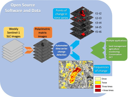
In this paper, we apply a polarimetric SAR-based time series change detection technique in two highly dynamic natural and semi-natural landscapes. We use a new method published in [16] where change detection is carried out by performing a simultaneous test of the hypothesis of homogeneity for a series of SAR images. Our research was conducted with three specific objectives in mind. First, we show the potential of using the time series change detection algorithm presented in [16] (referred to as S1-omnibus) and Sentinel-1 time series to capture short-term changes in highly dynamic areas. Second, we evaluate the performance of S1-omnibus vs. a pairwise comparison of consecutive images. According to [16], it is expected that a larger proportion of change will be detected using the whole time series as opposed to the commonly-used pairwise approach. Third, we compare the performance of S1-omnibus with a Landsat-based change detection approach. Since optical and SAR instruments detect different properties of objects, it cannot be considered as a validation process, but it is still relevant to compare the performance of the new S1-omnibus algorithm with more extended and common approaches.

2. Study Areas

Many wetlands experience several short-term changes mostly related to water surface dynamics (seasonal water bodies and water ways, intertidal flats, temporarily inundated forests, among others) or related to human activities, such as agriculture or salt production. To test the capacities of the S1-omnibus method, we chose two highly dynamic wetlands with different characteristics.

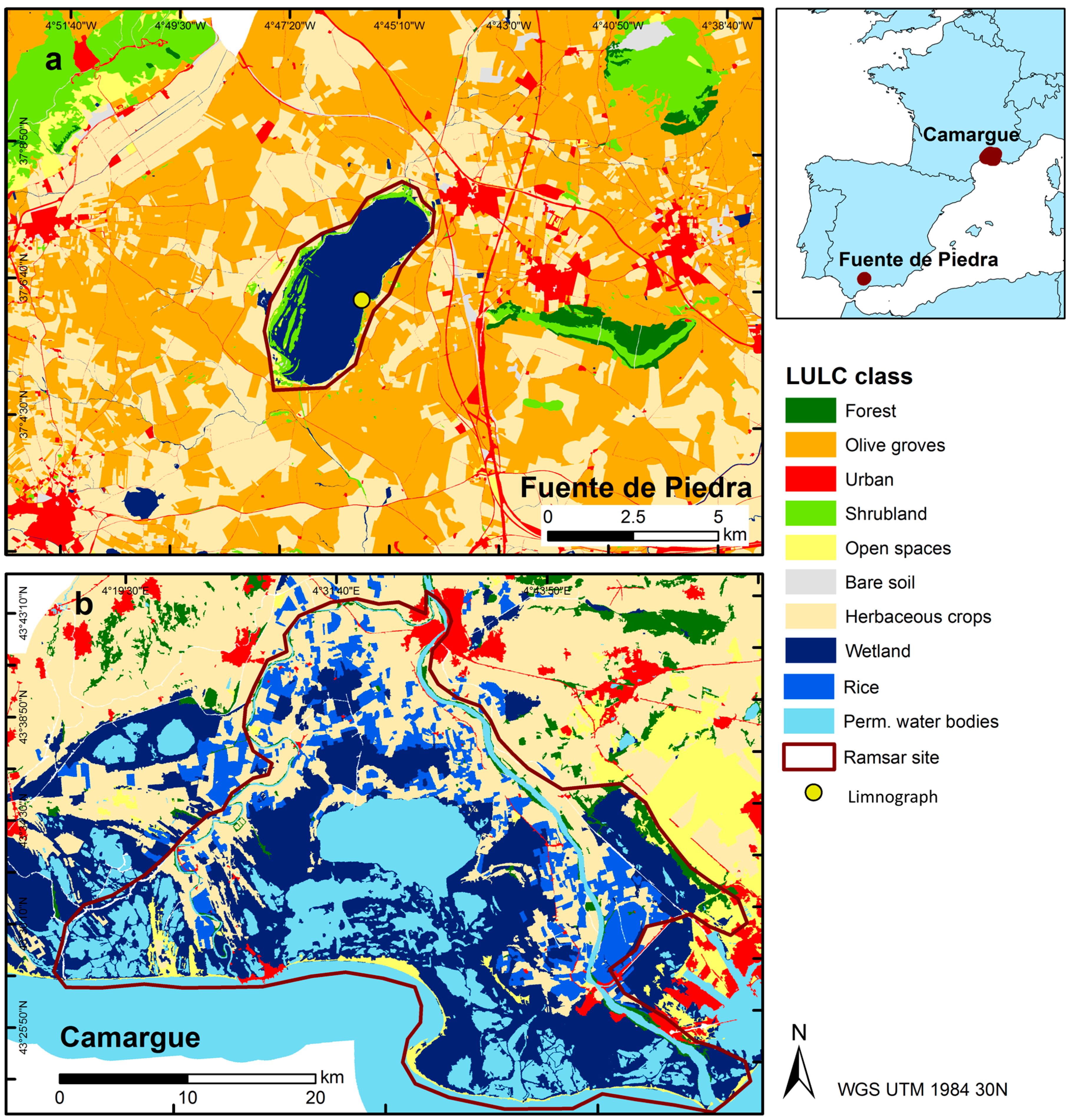
The first one is the Lagoon of Fuente de Piedra, in southern Spain: an endorheic salty lagoon of ~13 km² and less than 1 m deep. Its catchment occupies around 150 km², but we study all of the changes within a rectangular area of 490 km² (Figure 1). The lagoon is fed by two streams, although the most important supply of water is ground water inputs and rains [17]. Landscapes in the uplands are dominated by olive groves and herbaceous crops (e.g., wheat and barley), and the lagoon was used for salt extraction during the last century. Currently, it is a Ramsar site and a nature reserve. It usually dries out at the end of spring and fills up again with the first autumn rains. Despite its small size, it is a migratory stopover for many bird species and the second largest breeding ground in Europe for the European flamingo (Phoenicopterus roseus) [18].

The second study area is the largest flamingo breeding ground in Europe; the French Camargue. It is coastal wetland of 130 km² located in the south of France, between both arms of the Rhône River Delta. It belongs to a larger and complex system of coastal wetlands and lagoons that have been flooded, dredged, canaled and cultivated during many centuries. Currently, it is a Ramsar site and a national reserve, but water is still pumped in and out for salt production and for keeping some lagoons filled during summer in certain areas. The change detection method was applied to a rectangular area of 3500 km² (Figure 1). Landscapes are dominated by large permanent water bodies, rice fields and other crops, salt flats and marshes near the coast and pastures for extensive cattle. The salinity of the water bodies varies depending on the rain, but it generally increases from north to south. The deepest water body, the Vaccarés lagoon, in the center of the wetland, has a maximum depth of 2 m [19].

Both study areas are test sites of the SWOS project, which allowed access to ground information, as well as to mapping products that were used for the interpretation of the results (e.g., LULC maps from Figure 1). In these as in many other wetlands over the world, the presence/absence and quality of their water is influenced by land uses (mainly agricultural) in their area of hydric influence. Thus, we analyze not only the areas designated as wetland in our two study sites, but also their surroundings.

3. Materials and Methods

3.1. Imagery and Preprocessing

We used a set of several Sentinel-1 images from the ESA Scientific Data Hub acquired for 2014/2015 at a monthly resolution and with the same orbit path (

Table 1. Sentinel-1 and Landsat 7, 8 datasets used. Images used for the S1-omnibus and Landsat-based CVA change detection comparison are highlighted. Landsat 7 images are marked with an asterisk (*).

Fuente de Piedra (Spain)		Camargue (France)
Sentinel 1	Landsat	Sentinel 1	Landsat
		11 November 2014
		02 December 2014
		31 January 2015
		24 February 2015
15 March 2015	09 March 2015 *	08 March 2015
20 April 2015	02 April 2015	01 April 2015	15 April 2015
26 May 2015	12 May 2015 *	07 May 2015	17 May 2015
19 June 2015	05 June 2015	12 June 2015	02 June 2015
25 July 2015	07 July 2015	18 July 2015	20 July 2015
18 August 2015	16 August 2015 *	18 August 2015	21 August 2015
23 September 2015	25 September 2015	28 September 2015	06 September 2015
17 October 2015
22 November 2015	12 November 2015
28 December 2015
21 January 2016
26 February 2016

). Sentinel-1 imagery is offered in four different swath modes, three product types and with different polarization options. The swath mode used here is the Interferometric Wide (IW) swath, and the product type is the Single Look Complex (SLC), which consists of focused SAR data that uses the full C signal bandwidth and preserves the phase information. In the other product type for land masses, the Ground Range Detected (GRD), the phase information is lost, and thus, it cannot be used to produce the covariance matrix needed during the change detection. We used dual polarimetric images (VV-VH), which allow the measurement of the polarization properties of the terrain in addition to the backscatter that could be measured from a single polarization. The raw images were preprocessed in the Sentinel Application Platform (SNAP). The sub-swaths of the SLC image were split and de-bursted separately, and then, a 2 × 2 polarimetric matrix image was calculated. To reduce the speckle noise inherent to SAR data, a multilook spatial averaging was applied with 8 range looks and 2 azimuth looks. Finally, a terrain correction using 3 arcsec SRTM and bilinear interpolation was applied, resulting in an image with a nominal pixel size of 30 m × 30 m. The final polarimetric and multilooked matrix image that is used during the change detection has the form:

$$c2=\left(\begin{array}{cc}\langle {\left|S_{vv}\right|}^2\rangle & \langle S_{vv}{S}_{vh}^{*}\rangle \\ \langle S_{vh}{S}_{vv}^{*}\rangle & \langle {\left|S_{vh}\right|}^2\rangle \end{array}\right)$$

where $s_{tr}$ is the scattering amplitude for transmitted polarization t and received polarization r, $<\dots >$ denotes multilook averaging and v and h correspond to vertical and horizontal polarizations, respectively. When multiplied by the number of looks, the matrix c2 is known to follow a complex Wishart distribution parameterized by a covariance matrix ∑ [22].

3.2. SAR-Based Change Detection

The change detection algorithm applied in this research takes advantage of the known distributions of the observations c2. It detects changes within a series of k uncorrelated multilooked images by testing, pixel-wise, hypotheses on the values of the parameters ${{\displaystyle \sum }}_i, i=1\dots k$, characterizing the distributions. To test the null (no-change) hypothesis $H_0:{{\displaystyle \sum }}_1={{{\displaystyle \sum }}^{\text{}}}_2= \dots ={{{\displaystyle \sum }}^{\text{}}}_k$ against all alternative (change) hypotheses, we use an omnibus test statistic:

$$Q={\left[k^{2k}\frac{{{\displaystyle \prod }}_{i=1}^k\left|c{2}_i\right|}{{\left|C2\right|}^k}\right]}^n$$

where n is the number of looks and where $C2= {\displaystyle \sum }_{i=1}^{k}c{2}_i$. In order to set the significance for the test, the distribution of Q must be known. Approximate values are given in [16], the accuracy of which increases with the number of looks. We estimated the best equivalent number of looks to be 12, out of the total 16 (8 range × 2 azimuth). In addition, [16] derive a factorization of the test statistic Q, which allows the determination of the interval in which changes occur within the time series. Thus, we test, for example, the null hypothesis that, given ${{{\displaystyle \sum }}^{\text{}}}_1={{{\displaystyle \sum }}^{\text{}}}_2= \dots ={{{\displaystyle \sum }}^{\text{}}}_{j-1}$, it is also true that ${{{\displaystyle \sum }}^{\text{}}}_1={{{\displaystyle \sum }}^{\text{}}}_{j-1},$against the alternative that ${{{\displaystyle \sum }}^{\text{}}}_1\ne {{{\displaystyle \sum }}^{\text{}}}_{j-1}$. If the null hypothesis is rejected, the sequential testing procedure is restarted at the next observation. In this way, all time intervals in which changes occur can be identified.

To assess the capabilities of the omnibus time series change detection algorithm, we applied it to a series of consecutive Sentinel-1 images spanning one year (approximately one image per month; see Table 1). Using the same set of images, we compared the results of the S1-omnibus approach against the standard pairwise change detection approach, also based on the Wishart distribution [22]. All of the changes detected between pairs of consecutive images were summed up and compared. All changes are at the 1% significance level in the per pixel change hypothesis tests.

The analysis was performed using an innovative open source software implementation [23]. The python scripts for the change detection algorithms are encapsulated, together with all prerequisites, in a Docker container. No special software is required. The user interacts with the software in his or her browser in an IPhython notebook served from within the Docker container.

We used data from a limnograph and pluviometer placed towards the center-east of the lagoon in Fuente de Piedra to interpret the results of S1-omnibus.

3.3. S1-Based and Landsat-Based Change Detection Comparison

We used a smaller set of cloud-free Landsat 7 and 8 images acquired as closely as possible in time to the Sentinel-1 imagery for comparison purposes (Table 1). We performed an Iteratively Re-Weighted Multivariate Alteration Detection (IR-MAD) [24] to radiometrically adapt all of the Landsat images to the last one. Using Change Vector Analysis (CVA) [25], we extracted the changes between each pair of consecutive images and sum them up to create a Landsat-based change mask. Since there was not always a cloud-free Landsat image per Sentinel-1 image, for this comparison, we used only the Sentinel-1 images for which we had a corresponding cloudless Landsat image to create a Sentinel-1-based change mask and compare it to the Landsat-based change mask. This involved images from the period from March 2015–November 2015 for Fuente de Piedra, and from April 2015–November 2015 for Camargue. Table 1 shows detailed information about the images used for the different procedures. Due to the Scan Line Corrector failure in Landsat 7, images taken after June 2003 have no-data pixels along their edges, but the nadir of the scenes does not suffer such data loss. The test site of Fuente de Piedra is located at nadir, and thus, it was possible to use Landsat 7 images there. Only Landsat 8 images were used over the Camargue.

4. Results

4.1. S1-Omnibus Approach

S1-omnibus allows one to identify in time the changes detected within the time series. The output is a raster with one band per time interval analyzed (i.e., number of images −1). Each band contains the changes detected in each time interval. Figure 2 shows the results obtained for Fuente de Piedra in a closer look at the lagoon.

The changes detected in the outer part of the lagoon between March and April (Figure 2a) suggest that it starts drying there. Between April and May (Figure 2b), most of the lagoon dries out, which matches with the reduction in the water table recorded by the limnograph. No major changes are detected until October (Figure 2g), when the first autumn rains occur. These precipitations are not strong enough to raise the water table levels, but they seem to be enough to cause changes in the dry soils of the wetland. Note that the image from 17 October 2016 was taken right before major precipitations during 18 October 2016 (28.5 mm). Changes detected between October and November (Figure 2h), November and December (Figure 2i) and December and January (Figure 2j) match the records of the limnograph.

A second output of S1-omnibus is the frequency of short-term change (Figure 3). It shows where multiple changes have been detected and how many.

In Fuente de Piedra, the areas more prone to suffer changes are the herbaceous crops, as well as the wetland area. The northern part of the lagoon has experienced several changes (up to six), most of them during the rainy period (October–April), when the lagoon fills up and dries out several times, until it dries completely by June. Growth and harvest patterns of the different cereals grown are also detected, and the harvest frequency can be estimated. Crops in the northwestern corner seem to be the most intensively used. Olive groves, forests and shrublands remain unchanged through the year, as well as urban settlements. Similar change patterns can be spotted in Camargue (Figure 4). The marshlands to the south of the Vaccarés Lagoon exhibit multiple changes, up to eight in some areas. Some crops exhibit also very high rates of change, as well as some areas classified as urban tissue.

The rates of change found were grouped according to the LULC maps in both test sites (Figure 4). In Camargue, a large proportion of rice fields showed higher rates of change than other agricultural areas and also higher than wetlands. Forests, olive groves, shrublands and open spaces (areas with little or very sparse vegetation) showed the most static patterns.

4.2. Comparison of S1-Omnibus Time Series and Pairwise Change Detection Approaches

The S1-omnibus method detects more changes than the pairwise approach. In Fuente de Piedra, the S1-omnibus method classified as change an area of 114 km², compared to the 79 km² detected in the pairwise method (the whole analyzed area is a rectangular extension of 490 km²; Figure 1). Subsets A and B of Figure 5 show examples of the differences found between both approaches in areas of herbaceous crops in Fuente de Piedra. No changes were detected by the pairwise approach that were not also detected by S1-omnibus.

In Camargue, the S1-omnibus method also detected a larger proportion of change than the pairwise approach, creating more solid patches of change that correspond more to the vegetated object, whether it was a rice plot or natural herbaceous vegetation of the wetland. Other small sparse areas were reported as changed within large extensions of grasslands, changes that were not identified with the pairwise approach.

4.3. Landsat-Based and Sentinel-1-Based Change Detection Comparison

The comparison of S1-omnibus with Landsat-CVA change detection methods shows to a certain extent a good agreement (Figure 6), considering that optical and SAR sensors look at different properties of objects. As expected, using Sentinel-1 time series, one can detect a wider array of changes. Changes in water levels in the lagoon of Fuente de Piedra are detected equally well with Landsat and Sentinel-1. However, changes in certain areas of herbaceous crops are reported only by either Landsat or Sentinel-1 (Figure 6, Subsets A and B). In Fuente de Piedra, the total area reported as change by both Sentinel-1 and Landsat amounts to 56 km². On the other hand, the area reported as change only by either Landsat or by Sentinel-1 is 28 km² and 52 km², respectively (bar chart in Figure 6).

We performed the same S1-omnibus and Landsat-CVA comparison in Camargue, and the results were slightly different. S1-omnibus flagged as change an area of 424 km², and the Landsat-CVA reported change in 557 km². The area detected as change by both methods simultaneously has an extension of 250 km². The total area covers a rectangular extension of 3500 km².

5. Discussion

For effective land management and biodiversity conservation, it is essential to understand certain landscapes as mosaics of dynamic regimes rather than simplistic static cover types [7,8,9]. Temporarily-inundated wetlands belong to such category and require special approaches to assess their spatio-temporal dynamics. The statistically powerful approach we present uses free data and open source tools, which allows land planners and scientists to establish an automated and accurate monitoring service for short-term LULC change detection. We use the powerful factorization of the omnibus test statistic to perform unsupervised change analysis in two wetlands and detect areas and LULC classes of high change rates.

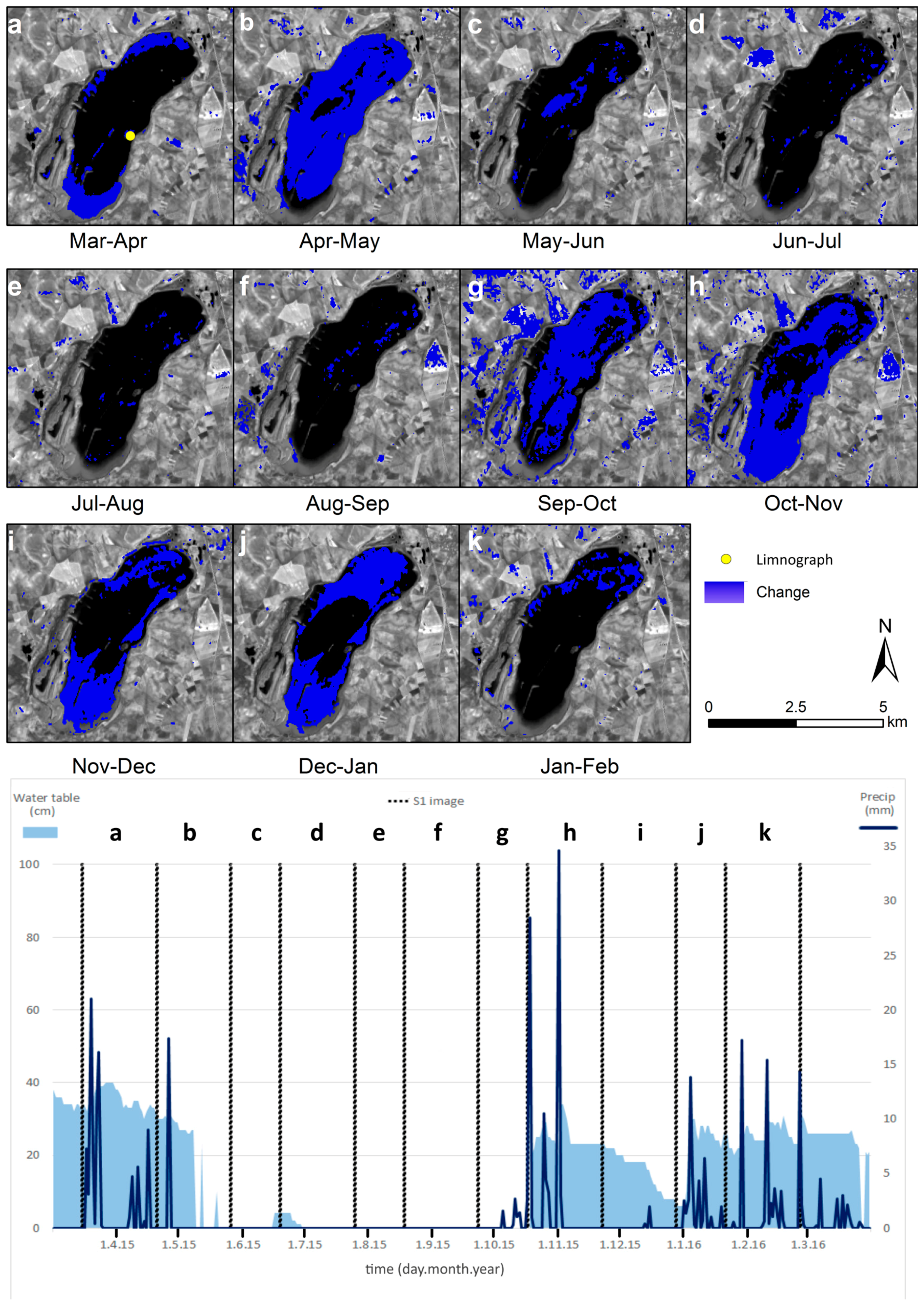
Locating the change patterns in space and time allows one to visualize change dynamics caused by variations in water flow or human activities. This enables us to estimate more precisely, for example, what areas dry out and when. Such estimations might be used in wetland wildlife management; breeding flamingos will abandon the single egg they lay if the wetland they are nesting in dries out too early or gets too flooded [26].

Limnographs and gauging stations have a very good temporal resolution, but poor spatial resolution. Combining these high cadence change maps with other in situ parameters, such as the ones given by limnographs, it is possible to improve hydrological models [27].

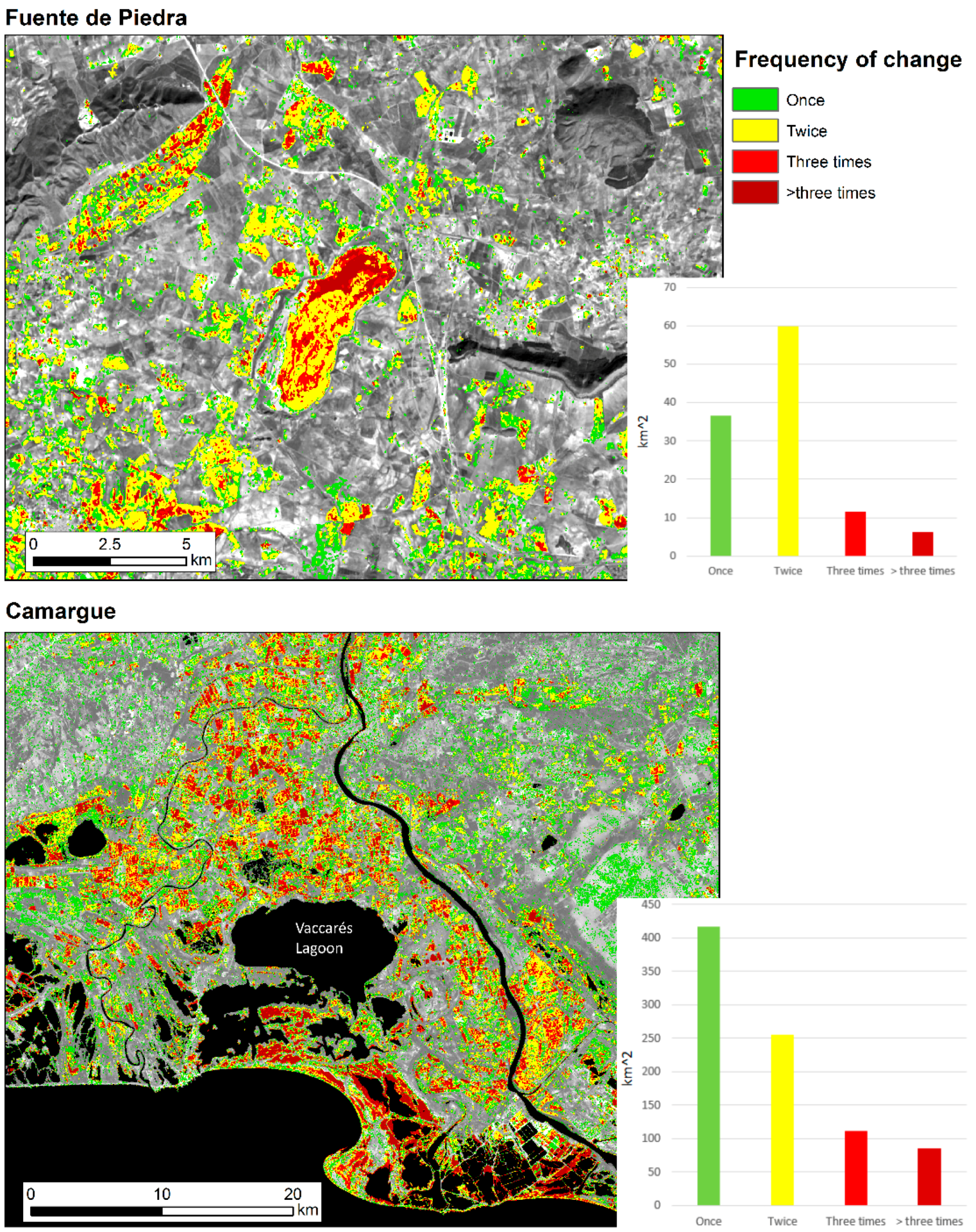
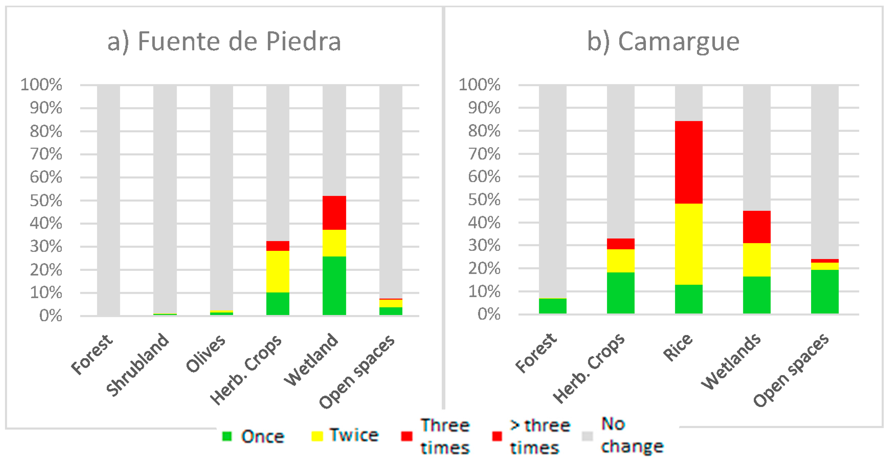
Maps depicting the frequency of change allow one to spot temporal and spatial patterns of short-term changes, as well as stable areas. For instance, the frequency of the change map in Fuente de Piedra shows high rates of change in the lagoon, as well as in some herbaceous crops, whereas olive groves, forest and natural shrublands remain mostly static throughout the year (Figure 3 and Figure 4). Most of the agricultural areas in Fuente de Piedra exhibit two changes, which suggest one harvest per year (one change from bare soil to crop and another one from crop to bare soil). Other areas of higher rates of change (three or more changes) can be spotted in agricultural areas northwest of the lagoon, suggesting several harvests per year.

In Camargue, high rates of change can be observed in the wetland south of the Vaccarés Lagoon, probably due to the influence of tides. False changes in permanent water bodies (e.g., the Mediterranean Sea) were reported when using Sentinel-1 in both approaches (i.e., S1-omnibus and the Sentinel-1 pairwise approach). Since these were not a real change and for a better visualization of the results, sea and other permanent water bodies were masked out in Figure 3 using a permanent water mask created out of a series of Landsat images for 2015. The reasons why SAR data report changes in permanent water bodies have yet to be studied, but this might be due to variations in the water table because of the tides or due to strong winds creating waves (Bragg scattering). Such changes were not detected in the Landsat images.

Change rates were grouped into LULC classes. This revealed two groups of classes: forests, olive groves and shrublands as more “static” classes and herbaceous crops, including rice fields and wetlands, as classes prone to suffer several changes throughout a year. This allows drawing estimations of land use. For example, during the period of study (one year), no changes were reported in around 70% of the area classified as herbaceous crops of both test sites. Although a field validation would be needed, this suggests that a large portion of the area destined to grow herbaceous crops other than rice may not be actually used, but remains fallow.

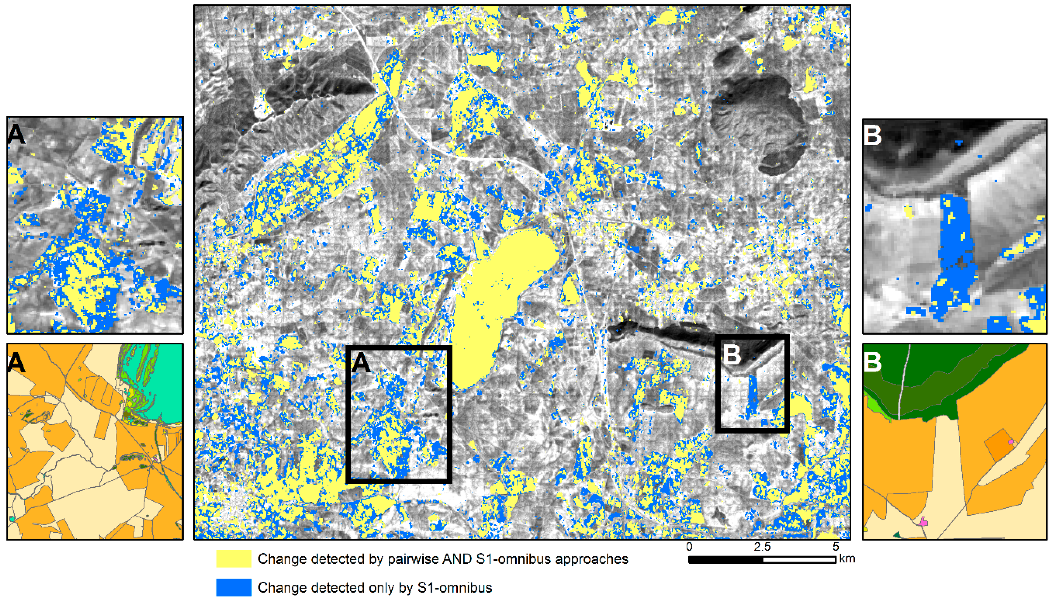
The S1-omnibus method reports a larger proportion of changes in the landscape than the pairwise approach in both study areas and in both agricultural and natural landscapes. As [16] suggested, detecting changes in consecutive pairs of images may leave undetected weak trends overtime, such as the slow growth of herbaceous vegetation after a disturbance, whether this is of anthropic origin, such as harvests, or of natural origin, like seasonal inundations. S1-omnibus seems to be able to detect these gradual changes.

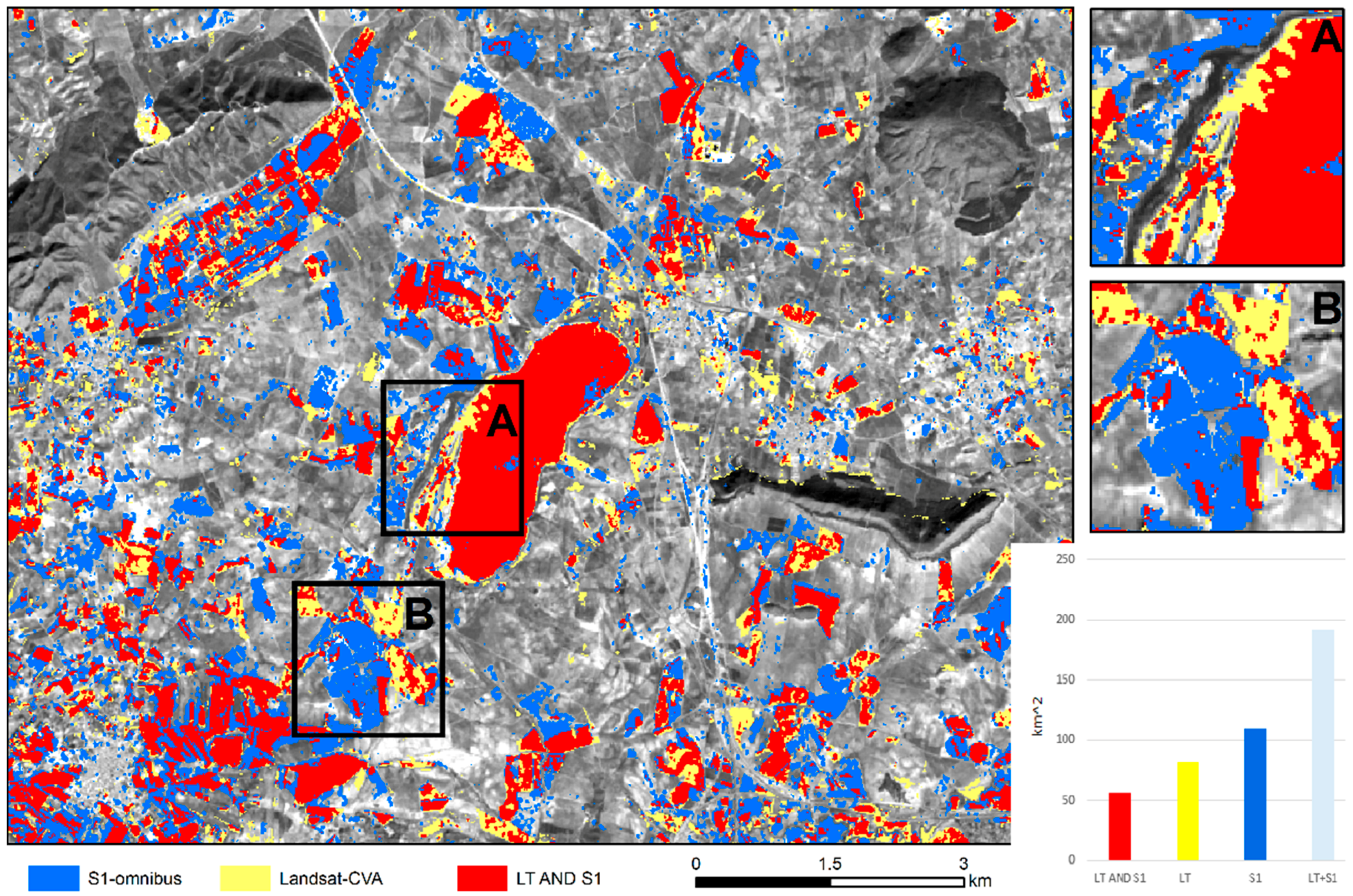
The comparison of S1-omnibus and Landsat-CVA showed generally good agreement in Fuente de Piedra, with changes in some patches of herbaceous crops missed by either of the methods (Figure 6). In Camargue, optical and SAR methods performed more differently. Landsat-CVA flagged as change a larger extent, mainly of herbaceous crops other than rice. This might be due to phenological changes in blooming vegetation that are difficult to detect with SAR imagery.

The comparison between the water table and precipitation data and the sequence of changes detected by S1-omnibus (Figure 2) reveal how important it is to have a high cadence of imagery to capture all of the changes produced in such dynamic ecosystems. We limited our research to one Sentinel-1 image per month (every 24 or 36 days) for simplification purposes, but with the recent launch of Sentinel-1B, it is now possible to map these dynamics every six days. It would not be possible to reach even a similar cadence using optical data. Although both study areas are relatively cloud-free throughout the year, we could only find 6–8 cloud-free Landsat scenes for our test sites, all restricted to the dry period. The lack of suitable optical images is greater for larger areas (the larger the area is, the more probable it is to find clouds in it), during rainy seasons and especially in the sub-humid and humid tropics. Some events, like fast floods or flooding of certain creeks or ponds, may take place only during the rainy season.

Potentials and Limitations of the Application

Although S1-omnibus cannot directly provide information on the type of change, this approach can still be useful for land managers with local knowledge or in situ data that allow them to interpret the changes and change rates. Knowing the short-term change patterns of certain land covers may aid in their classification, especially when classifying different types of wetlands, since some of them are defined by their dynamics. For instance, wet meadows are defined by seasonally- or temporally-saturated soils and brief periods of inundation [7]. Such periods of inundation can be accurately mapped using Sentinel-1 time series in order to define subclasses of wetlands and further describe the ecological status and condition of DCT. The increased temporal resolution of Sentinel-1 time series provides an information source for a better physically-based characterization of wetland types following a standardized nomenclature, e.g., Ramsar, or the Mapping and Assessment of Ecosystems and their Services (MAES). Integrating the S1-omnibus approach in operational wetland mapping activities fosters a more systematic monitoring of wetland dynamics. The broad change results thus provide a very flexible application for analyzing specific hydrological or plant phenology-driven analyses at very local scales.

Dual pol SAR data have been used before to monitor grass cutting practices for biodiversity management and subsidy control purposes, but the number of studies available is limited [28]. In fields of tall grass, meteorological conditions such as wind can influence the backscatter signal, reporting a change when there was actually none [28]. In a pairwise comparison of consecutive images, it is difficult to remove such influence, but it may be possible to filter that noise out by applying S1-omnibus; if using time series with a high temporal resolution, (e.g., weekly), the algorithm could be modified so that if ${{{\displaystyle \sum }}^{\text{}}}_1\ne {{{\displaystyle \sum }}^{\text{}}}_2$, but ${{{\displaystyle \sum }}^{\text{}}}_1={{{\displaystyle \sum }}^{\text{}}}_3$, the change reported between ${{{\displaystyle \sum }}^{\text{}}}_1$ and ${{{\displaystyle \sum }}^{\text{}}}_2$ could be flagged as a false positive.

The different changes recorded by Landsat-CVA and S1-omnibus show the potential of combining optical and SAR sensors for change detection. Sentinel-1-based change detection can also be combined with other sensors to determine the direction of change and to create a change mask to reduce error propagation in the labeling phase of the production of long-term LULCC maps [11].

Sentinel-1 does not always acquire dual-pol images, and for certain parts of the globe during certain periods, only single polarization (VV) images are available. Information on the schedule of different acquisition modes can be found at https://sentinel.esa.int/web/sentinel/missions/sentinel-1/observation-scenario. We also tested the S1-omnibus approach with single-pol VV Sentinel-1 images, and the results looked promising, but the accuracy has yet to be evaluated. An important limitation is the inherent low vegetation canopy penetration of C-band. This hinders its application for wet forests and mangroves, for which an L-band sensor would be more suitable.

It is still necessary to determine with more exactitude the change detection capabilities of S1-omnibus; e.g., how tall/thick the vegetation must be for it to be detected when it is removed or grows. Additional work to validate this change detection methodology with time series is underway using a variety of test sites where we have a higher level of control.

The open source character of our approach allows its incorporation with other tools where dense time series may be used, such as Google Earth Engine or the future SWOS portal and toolbox, which in turn may increase the number of applications of the S1-omnibus.

6. Conclusions

SAR-based change detection approaches offer a great opportunity to enhance our understanding of complex and dynamic ecosystems. S1-omnibus is capable of capturing accurately in space and time a wide array of LULC changes, and along with Sentinel-1 time series, it is possible to reach a six-day cadence at 30-m resolution. We demonstrate its potential for wetland monitoring by mapping change patterns caused by surface water dynamics and agricultural practices for a one-year period. Coupled with ground data like gauging stations, S1-omnibus and Sentinel-1 time series can be used to improve hydrological models [27]. Wetland managers can easily interpret the patterns of change and use them to locate and delineate areas of high rates of change, which are prone to have a high ecological value [8,9]. Incorporating a temporal variable into the LULC classification procedures may allow the separation of land cover categories that, to this date, have proven difficult. The S1-omnibus’s statistical soundness, higher control of false negatives and false positives [16] and the fact that it does not require complex parameterization make it an ideal method for operational monitoring services. We also demonstrate its advantages against standard change detection approaches that use pair-wise comparisons of SAR and optical images.

References

1. Mitsch, W.J.; Gosselink, J.G. The value of wetlands: Importance of scale and landscape setting. Ecol. Econ. 2000, 35, 25–33. [Google Scholar] [CrossRef]
2. Tiner, R. Introduction to wetland mapping and its challenges. In Remote Sensing of Wetlands; Tiner, R., Lang, M., Klemas, V., Eds.; CRC Press: Boca Raton, FL, USA, 2015; pp. 43–66. [Google Scholar]
3. Henderson, F.M.; Lewis, A.J. Radar detection of wetland ecosystems: A review. Int. J. Remote Sens. 2008, 29, 5809–5835. [Google Scholar] [CrossRef]
4. Brisco, B.; Schmitt, A.; Murnaghan, K.; Kaya, S.; Roth, A. SAR polarimetric change detection for flooded vegetation. Int. J. Digit. Earth 2013, 6, 103–114. [Google Scholar] [CrossRef]
5. Coppin, P.; Jonckheere, I.; Nackaerts, K.; Muys, B.; Lambin, E. Review ArticleDigital change detection methods in ecosystem monitoring: A review. Int. J. Remote Sens. 2004, 25, 1565–1596. [Google Scholar] [CrossRef]
6. Reschke, J.; Hüttich, C. Continuous field mapping of Mediterranean wetlands using sub-pixel spectral signatures and multi-temporal Landsat data. Int. J. Appl. Earth Obs. Geoinf. 2014, 28, 220–229. [Google Scholar] [CrossRef]
7. Dronova, I.; Gong, P.; Wang, L.; Zhong, L. Mapping dynamic cover types in a large seasonally flooded wetland using extended principal component analysis and object-based classification. Remote Sens. Environ. 2015, 158, 193–206. [Google Scholar] [CrossRef]
8. Parrott, L.; Meyer, W.S. Future landscapes: Managing within complexity. Front. Ecol. Environ. 2012, 10, 382–389. [Google Scholar] [CrossRef]
9. Watson, S.J.; Luck, G.W.; Spooner, P.G.; Watson, D.M. Land-use change: Incorporating the frequency, sequence, time span, and magnitude of changes into ecological research. Front. Ecol. Environ. 2014, 12, 241–249. [Google Scholar] [CrossRef]
10. Lu, D.; Mausel, P.; Brondízio, E.; Moran, E. Change detection techniques. Int. J. Remote Sens. 2004, 25, 2365–2401. [Google Scholar] [CrossRef]
11. Hecheltjen, A.; Thonfeld, F.; Menz, G. Recent advances in remote sensing change detection—A review. In Land Use and Land Cover Mapping in Europe; Manakos, I., Braun, M., Eds.; Springer: Dordrecht, The Netherlands, 2014; Volume 18, pp. 145–178. [Google Scholar]
12. Nguyen, D.; Clauss, K.; Cao, S.; Naeimi, V.; Kuenzer, C.; Wagner, W. Mapping rice seasonality in the Mekong delta with multi-year Envisat ASAR WSM data. Remote Sens. 2015, 7, 15868–15893. [Google Scholar] [CrossRef]
13. Bouvet, A.; le Toan, T. Use of ENVISAT/ASAR wide-swath data for timely rice fields mapping in the Mekong River Delta. Remote Sens. Environ. 2011, 115, 1090–1101. [Google Scholar] [CrossRef] [Green Version]
14. SWOS|Satellite-Based Wetland Observation Service. Available online: http://www.swos-service.eu/ (accessed on 30 May 2016).
15. GEO—Group on Earth Observations. Available online: https://www.earthobservations.org/index.php (accessed on 30 May 2016).
16. Conradsen, K.; Nielsen, A.A.; Skriver, H. Determining the points of change in time series of Polarimetric SAR Data. IEEE Trans. Geosci. Remote Sens. 2016, 54, 3007–3024. [Google Scholar] [CrossRef]
17. Conde-Álvarez, R.M.; Bañares-España, E.; Nieto-Caldera, J.M.; Flores-Moya, A.; Figueroa, F.L. Submerged macrophyte biomass distribution in the shallow saline lake Fuente de Piedra (Spain) as function of environmental variables. Anales del Jardín Botánico de Madrid 2012, 69, 119–127. [Google Scholar] [CrossRef]
18. Geraci, J.; Béchet, A.; Cézilly, F.; Ficheux, S.; Baccetti, N.; Samraoui, B.; Wattier, R. Greater flamingo colonies around the Mediterranean form a single interbreeding population and share a common history. J. Avian Biol. 2012, 43, 341–354. [Google Scholar] [CrossRef]
19. Britton, R.H.; Podlejski, V.D. Inventory and classification of the wetlands of the Camargue (France). Aquat. Bot. 1981, 10, 195–228. [Google Scholar] [CrossRef]
20. Descargar SIOSE. Available online: http://www.siose.es/descargar (accessed on 30 May 2016).
21. Tour du Valat. Available online: http://www.tourduvalat.org/ (accessed on 30 May 2016).
22. Conradsen, K.; Nielsen, A.A.; Schou, J.; Skriver, H. A test statistic in the complex wishart distribution and its application to change detection in polarimetric SAR data. IEEE Trans. Geosci. Remote Sens. 2003, 41, 4–19. [Google Scholar] [CrossRef] [Green Version]
23. SARDocker by Mortcanty. Available online: http://mortcanty.github.io/SARDocker/ (accessed on 30 May 2016).
24. Canty, M.J.; Nielsen, A.A. Automatic radiometric normalization of multitemporal satellite imagery with the iteratively re-weighted MAD transformation. Remote Sens. Environ. 2008, 112, 1025–1036. [Google Scholar] [CrossRef]
25. Malila, W.A. Change vector analysis: An approach for detecting forest changes with Landsat. In LARS Symposia; Laboratory for Applications of Remote Sensing: West Lafayette, IN, USA, 1980. [Google Scholar]
26. Béchet, A.; Germain, C.; Sandoz, A.; Hirons, G.J.M.; Green, R.E.; Walmsley, J.G.; Johnson, A.R. Assessment of the impacts of hydrological fluctuations and salt pans abandonment on Greater flamingos in the Camargue, South of France. Biodivers. Conserv. 2009, 18, 1575–1588. [Google Scholar] [CrossRef]
27. Wdowinski, S.; Hong, S.-H. Wetland InSAR: A review of the technique and applications. In Remote Sensing of Wetlands; Tiner, R., Lang, M., Klemas, V., Eds.; CRC Press: Boca Raton, FL, USA, 2015; pp. 137–154. [Google Scholar]
28. Voormansik, K.; Jagdhuber, T.; Olesk, A.; Hajnsek, I.; Papathanassiou, K.P. Towards a detection of grassland cutting practices with dual polarimetric TerraSAR-X data. Int. J. Remote Sens. 2013, 34, 8081–8103. [Google Scholar] [CrossRef]
Figure 1. LULC maps of the study areas (a,b). In Fuente de Piedra (a), the classification has been performed using photointerpretation and field inventories [20]. The classification in Camargue (b) is a product of the project SWOS, elaborated by Tour du Valat using Landsat images for 2015 and field inventories [21]. In order to make both classification compatible and for the sake of simplification, some classes have been merged, e.g., the class “wetlands” includes marshlands, temporal water bodies and salt marshes; “open spaces” includes areas with little vegetation, dunes and some pastures; “urban” includes all sorts of pavement or concrete; “forests” includes coniferous, as well as broad-leaved forests.
Remotesensing 08 00795 g001
Figure 2. Month by month changes detected by S1-omnibus in the Lagoon of Fuente de Piedra marked with letters (ak) in the upper left corner of each image. Their corresponding water table and precipitation levels can be found in the chart. Water table and precipitations were recorded by a limnograph and pluviometer at the center of the lagoon, marked with a yellow circle in “a”. The same Landsat 8 band 4 image has been used as the background in (ak).
Remotesensing 08 00795 g002
Figure 3. Frequency of change in Fuente de Piedra and Camargue. Colors indicate how many times a pixel has changed over the 12-month period. The charts aggregate the frequencies of change by area (Landsat 8 band 4 used as the background image).
Remotesensing 08 00795 g003
Figure 4. Frequencies of change aggregated in LULC classes in Fuente de Piedra (a) and Camargue (b). Each chart accounts for the proportion of pixels of each LULC class where a change was detected once, twice, three or four or more times. The gray portion of the bar corresponds to areas where no change was detected.
Remotesensing 08 00795 g004
Figure 5. Changes detected in Fuente de Piedra by the pairwise change detection approach (yellow) overlaid on top of the S1-omnibus change detection results (blue). Changes in water level and in most crops are well detected by both approaches. Subset A shows how the S1-omnibus is capable of detecting changes in patches of crops matching the LULC map better (in the LULC map, orange is olive groves and beige herbaceous crops); Subset B shows how S1-omnibus can even detect whole patches of change that are missed with the pairwise approach (Landsat 8 band 4 used as the background image).
Remotesensing 08 00795 g005
Figure 6. Changes detected by S1-omnibus (blue), by Landsat-CVA (yellow) and by both methods (red). Subsets A and B show a closer look at the two areas of change indicated in the main image. In chart, light blue color represents the area detected as change by either method.
Remotesensing 08 00795 g006