Spatially and Temporally Complete Satellite Soil Moisture Data Based on a Data Assimilation Method

Abstract

Multiple soil moisture products have been generated from data acquired by satellite. However, these satellite soil moisture products are not spatially or temporally complete, primarily due to track changes, radio-frequency interference, dense vegetation, and frozen soil. These deficiencies limit the application of soil moisture in land surface process simulation, climatic modeling, and global change research. To fill the gaps and generate spatially and temporally complete soil moisture data, a data assimilation algorithm is proposed in this study. A soil moisture model is used to simulate soil moisture over time, and the shuffled complex evolution optimization method, developed at the University of Arizona, is used to estimate the control variables of the soil moisture model from good-quality satellite soil moisture data covering one year, so that the temporal behavior of the modeled soil moisture reaches the best agreement with the good-quality satellite soil moisture data. Soil moisture time series were then reconstructed by the soil moisture model according to the optimal values of the control variables. To analyze its performance, the data assimilation algorithm was applied to a daily soil moisture product derived from the Advanced Microwave Scanning Radiometer for the Earth Observing System (AMSR-E), the Microwave Radiometer Imager (MWRI), and the Advanced Microwave Scanning Radiometer 2 (AMSR2). Preliminary analysis using soil moisture data simulated by the Global Land Data Assimilation System (GLDAS) Noah model and soil moisture measurements at a multi-scale Soil Moisture and Temperature Monitoring Network on the central Tibetan Plateau (CTP-SMTMN) was performed to validate this method. The results show that the data assimilation algorithm can efficiently reconstruct spatially and temporally complete soil moisture time series. The reconstructed soil moisture data are consistent with the spatial precipitation distribution and have strong positive correlations with the values simulated by the GLDAS Noah model over large areas of the region. Compared to the soil moisture measurements at the medium and large networks, the reconstructed soil moisture data have almost the same accuracy as the soil moisture product derived from AMSR-E/MWRI/AMSR2 for ascending and descending orbits.

1. Introduction

Soil moisture is one of the key parameters for the environment and climate system. It influences hydrological and agricultural processes and also impacts the climate system through atmospheric feedback loops. Conventional soil moisture observations made at a single localized point are too sparse to satisfy many research and application purposes.

Due to the penetrability of low frequency microwave signals through atmosphere, vegetation and superficial soil layer, microwave remote sensing has become one of the most useful tools for obtaining surface soil moisture data at regional and global scales [1,2]. Currently, multiple soil moisture products have been generated from data acquired by the Advanced Microwave Scanning Radiometer (AMSR-E) onboard the Aqua satellite [3], the Advanced Microwave Scanning Radiometer 2 (AMSR2) onboard the GCOM-W satellite [4], the Microwave Imaging Radiometer with Aperture Synthesis (MIRAS) onboard the Soil Moisture and Ocean Salinity (SMOS) satellite [1], and the Advanced Scatterometer (ASCAT) onboard the MetOP-A satellite [2]. A number of studies have assessed satellite soil moisture products through inter-comparisons with model simulations or other satellite soil moisture product [5,6,7,8,9], while other evaluation activities were performed against ground-based measurements [10,11,12,13,14,15]. However, current soil moisture products are not spatially or temporally complete [16]. The major reasons causing data gaps in these soil moisture products include track changes, radio-frequency interference, dense vegetation, and frozen soil. The presence of data gaps limits the application of soil moisture in land surface process simulation, climatic modeling, and global change research. Therefore, spatially and temporally complete soil moisture datasets are urgently needed nowadays for many practical applications [17].

Several methods have been used to fill gaps in remotely sensed data in recent years [18,19,20,21]. Generally speaking, these methods can be divided into two categories. The first involves smoothing and gap-filling in the time domain, mainly by asymmetric Gaussian function fitting [22], weighted least-squares linear regression [23], or a Savitzky-Golay (SG) filter [24]. The second involves smoothing and gap-filling in the frequency domain, e.g., the fitting method using a Fourier function [25]. These methods have been used mainly to restore normalized difference vegetation index (NDVI), leaf area index (LAI) [26], and albedo profiles [27]. Wang et al. [16] introduced a penalized least-squares method based on three-dimensional discrete cosine transforms for the purpose of filling data gaps in a global soil moisture product derived from satellite images. The method takes into account the full three-dimensionality of the spatio-temporal dataset and is an efficient way to fill data gaps in the rapidly growing volume and diversity of satellite datasets [16]. However, by using only statistical relationships for soil moisture data in space and time, the method does not consider the impact of precipitation and other factors on soil moisture changes when filling data gaps in soil moisture products.

To facilitate studies at a regional scale, some efforts have been made to simulate soil moisture using land surface models forced with precipitation and other atmospheric data. The Global Land Data Assimilation System (GLDAS) provides simulated soil moisture data at 1.0° and 0.25° resolution [28]. The simulated soil moisture data provide spatially and temporally consistent time series, but their accuracy is hindered by model deficiencies, and uncertainties in both model parameters and atmospheric forcing variables [14,29]. Recently, many studies have focused on the data assimilation of satellite observations into land surface models in attempt to produce optimal soil moisture estimates [30,31,32].

This study has developed a data assimilation method to assimilate satellite soil moisture into a soil moisture model and to generate spatially and temporally complete soil moisture data. Meteorological data were used to force the soil moisture model to simulate soil moisture data over time. The control variables of the soil moisture model were estimated from good-quality satellite soil moisture data covering one year. Soil moisture time series were then reconstructed by the soil moisture model according to the optimal values of the control variables. The data assimilation method was applied to a daily soil moisture product derived from AMSR-E, the Microwave Radiometer Imager (MWRI) onboard the FengYun-3B satellite, and AMSR2. The results were compared with the GLDAS soil moisture data simulated by the Noah model and with soil moisture measurements on the central Tibetan Plateau.

This paper is organized as follows. Section 2 introduces the proposed approach for reconstructing soil moisture time series. This includes the soil moisture model and soil moisture reconstruction. The meteorological data used to force the soil moisture model and the satellite soil moisture product used in this study are also briefly described in this section. Section 3 presents the results of the reconstructed soil moisture time series using the proposed method and a comparison of these results with the GLDAS soil moisture data simulated by the Noah model and with soil moisture measurements on the central Tibetan Plateau. Discussions are presented in Section 4, and the final section provides brief conclusions.

2. Methodology and Data

The data assimilation method developed in this study used good-quality satellite soil moisture data covering one year to estimate the initial state variables and model parameters of a soil moisture model. Soil moisture data over time are simulated by the soil moisture model. The method tunes the control variables of the soil moisture model until the temporal behavior of simulated soil moisture reaches the best agreement with the multi-temporal satellite soil moisture data with good-quality. Then the daily soil moisture for the year is reconstructed by the soil moisture model according to the optimal values of the control variables. Detailed descriptions of some important parts of the new algorithm are provided below.

2.1. Soil Moisture Model

Assume that the surface soil layer of thickness D is a lumped system. Accordingly, the following water content balance equation can be used to simulate soil moisture in the soil layer for time period t [33,34]:

$$\frac{dw\left(t\right)}{dt}=f\left(t\right)-e\left(t\right)-g\left(t\right)\text{ and }w\left(t\right)<w_{\max }$$

(1)

where $w\left(t\right)$ is the soil moisture in millimeters, $f\left(t\right)$ is the fraction of precipitation infiltrating into the soil, $e\left(t\right)$ is the evapotranspiration component, $g\left(t\right)$ is the drainage component due to deep percolation, and $w_{\max }$ is the maximum water capacity of the soil layer.

The fraction of precipitation infiltrating into the soil can be estimated using the following empirical equation [33,34]:

$$f\left(t\right)=p\left(t\right)\times \left(1-{\left(\frac{w\left(t\right)}{w_{\max }}\right)}^m\right)$$

(2)

where $p\left(t\right)$ is the precipitation in millimeters and $m$ is a parameter linked to the nonlinearity of the infiltration process.

The drainage component due to deep percolation is a nonlinear function of $w\left(t\right)$ [33,34]:

$$g\left(t\right)=k_s\times {\left(\frac{w\left(t\right)}{w_{\max }}\right)}^{3+2/\mathsf{\lambda }}$$

(3)

where $\mathsf{\lambda }$ is a pore size distribution index linked to the structure of the soil layer and $k_s$ is the field-saturated hydraulic conductivity. This equation assumes that the water flow through the soil layer is a gravity driven flow.

The evapotranspiration component is calculated using the following equation [33]:

$$e\left(t\right)=e{t}_p\left(t\right)\times \frac{w\left(t\right)}{w_{\max }}$$

(4)

where $e{t}_p\left(t\right)$ is the potential evapotranspiration (mm·day⁻¹) calculated using the Turc method [35]:

$$e{t}_p\left(t\right)=0.013\times \mathsf{\alpha }\times \frac{T_{\text{mean}}}{T_{\text{mean}}+15}\times \frac{23.8856\times R_s+50}{\mathsf{\gamma }}$$

(5)

where $T_{\text{mean}}$ is the daily mean air temperature (°C), $R_s$ is the daily solar radiation (MJ·m⁻²·day⁻¹), $\mathsf{\alpha }$ is a humidity-based value, and $\mathsf{\gamma }$ is the latent heat of vaporization (MJ·kg⁻¹). $\mathsf{\alpha }$ is calculated as follows [33]:

$$\mathsf{\alpha }=\{\begin{array}{ll}1.0,& r{h}_{\text{mean}}\ge 50\\ 1+\frac{50-r{h}_{\text{mean}}}{70},& r{h}_{\text{mean}}<50\end{array}$$

(6)

where $r{h}_{\text{mean}}$ is the daily mean relative humidity (%). The daily solar radiation was estimated using the Hargreaves model [36,37]:

$$R_s=k_{rs}\times \sqrt{\left(T_{\max }-T_{\min }\right)}\times R_a$$

(7)

where $k_{rs}$ is an adjustment coefficient, $T_{\max }$ and $T_{\min }$ are the daily maximum and minimum air temperatures (°C), and $R_a$ is the extraterrestrial radiation (MJ·m⁻²·day⁻¹) determined from latitude and the time of the year and was calculated by using the equations given in Allen et al. [38].

The soil moisture model has five parameters ($w_{\max }$, $m$, $\mathsf{\lambda }$, $k_s$, and $k_{rs}$). The model simulations also require an initial soil moisture value ($w_0$), which can considerably influence the simulated soil moisture values. In this study, the moisture model was applied using a daily time step. The model parameters and the initial soil moisture value were taken as control variables for which optimal values were determined according to the soil moisture values retrieved from satellite observations. The optimal values of the control variables were then used to reconstruct the daily soil moisture time series.

2.2. Cost Function and Optimization Method

In this study, a variational data assimilation technique was used to estimate the control variables of the soil moisture model from time-series soil moisture retrieved from satellite observations. The soil moisture model is used to simulate soil moisture at each point in time corresponding to satellite observations over one year. The variational data assimilation technique consists of adjusting the values of the control variables of the soil moisture model so that the soil moisture values simulated by the soil moisture model optimally match the soil moisture retrieved from satellite observations, i.e., to minimize the following functional:

$$J\left(x\right)={\displaystyle \sum _{i=1}^n{\left(y_i-w_i\left(x\right)\right)}^2}$$

(8)

where i represents the time index, y_i the surface soil moisture retrieved from satellite observation at time step i. $w_i(\cdot )$ represents the soil moisture model described above, and the vector x depicts the parameter set to be estimated. In this study, x includes the five parameters of the soil moisture model and the initial soil moisture value.

To minimize the objective function J(x), the shuffled complex evolution optimization method, developed at the University of Arizona (SCE-UA), was used to obtain the optimal control vector. This method does not require the derivatives of the function and can avoid being trapped by small pits and bumps on the function surface. The SCE search routine is a global optimization strategy that combines the strength of the simplex method with the concepts of a controlled random search, competitive evolution, and the strategy of complex shuffling. The synthesis of these four concepts makes the SCE-UA method more effective, robust, flexible and efficien,t and less sensitive to initial parameter values than the simplex method [39].

2.3. Data

2.3.1. Meteorological Data

Meteorological data were used to force the soil moisture model. The meteorological variables required by the soil moisture model include daily maximum temperature, daily minimum temperature, daily mean temperature, daily mean relative humidity, and daily total precipitation. This study used the meteorological data generated by the CMA Land Data Assimilation System Version 1.0 (CLDAS-V1.0) [40]. The meteorological data were generated by fusing the ground measurements, satellite observations, and numerical model products using data fusion and assimilation techniques. The coverage of the meteorological data was the East Asian region (0°–60°N, 70°E–150°E). The spatial resolution of the meteorological data was 1/16° × 1/16°, and the temporal resolution was one hour.

The hourly temperature data were used to calculate the daily maximum temperature, daily minimum temperature, and daily mean temperature. The hourly precipitation data were used to calculate the daily total precipitation. CLDAS-V1.0 provides specific humidity data, which were converted to the relative humidity values required by the soil moisture model used in this study by means of the following equation [41]:

$$rh=\frac{q}{qs}\times 100$$

(9)

where rh is relative humidity (%), q is specific humidity (g/g), and qs is the saturation-specific humidity (g/g), which can be calculated as [41]:

$$qs=\frac{0.62197\times es}{p-0.378\times es}$$

(10)

where p is air pressure in kilopascals and es is the saturation vapor pressure in kilopascals, which can be calculated by using an approximate equation [41]:

$$es=6.1078\times e^{\frac{17.269\times T}{273.16+T-35.86}}$$

(11)

where T is air temperature in degrees Celsius.

The meteorological data were aggregated to a 0.25° spatial resolution used in the following soil moisture product with a spatial-average method. The aggregated meteorological data were used to force the soil moisture model.

2.3.2. Soil Moisture Data

Based on zero-order radiative transfer theory and the Qp model [42], Liu et al. [43] proposed a two-channel retrieval algorithm to retrieve soil moisture from AMSR-E, which was validated in the Tibet region. The method was used to generate a global soil moisture product for the period 2002–2013 based on observations from AMSR-E (June 2002–September 2011) and similar sensors, including MWRI (October 2011–June 2012) and AMSR2 (July 2012–December 2013). To ensure consistent observations over different sensors, an inter-sensor calibration technique proposed in [44] was used to calibrate AMSR2 and MWRI brightness temperature datasets. The soil moisture product was provided in a geographic latitude/longitude projection at a spatial resolution of 0.25° (about 25 km at the Equator) and a daily temporal resolution. For clarification, the soil moisture product derived by the two-channel retrieval algorithm is denoted by TCRM. Jiang et al. [45] and Liu et al. [43] report that the accuracy of the TCRM soil moisture product is much better than that of other existing soil moisture products from AMSR-E, including the NASA standard soil moisture product [46], the Japan Aerospace Exploration Agency (JAXA) soil moisture product [4], and both the C-band and X-band soil moisture products developed using the Land Parameter Retrieval Model [47]. In this study, the TCRM soil moisture product for 2012 over the same area as the meteorological data (0°–60°N, 70°E–150°E) was used for testing the algorithm. Surface soil moisture is positively correlated with subsequent precipitation. Therefore, the TCRM soil moisture values are assumed to be of good quality in this work when both the soil moisture values and the precipitation are greater than their respective annual averages. At the same time, the soil moisture values are also considered to be of good quality when both the soil moisture values and the precipitation are less than their respective annual averages. Only the TCRM soil moisture with good-quality for the year was used to reconstruct spatially and temporally complete soil moisture data.

The Global Land Data Assimilation System was developed to generate optimal fields of land surface states and fluxes by integrating satellite- and ground-based observational data products, using land surface modeling and data assimilation techniques [28]. GLDAS data are archived and distributed on the Web site of the Goddard Earth Sciences Data and Information Services Center [48]. In this study, the three-hourly 0.25° soil moisture data simulated by the Noah model were used to evaluate the spatial consistency of the reconstructed soil moisture data. The Noah model provides depth-averaged soil moisture values in four different vertical soil layers with depths of 0–10, 10–40, 40–100, and 100–200 cm. To achieve a better depth match between the soil moisture values retrieved from satellite observations and those simulated by the Noah model, the satellite soil moisture was evaluated against the values for the first layer of the Noah model (0–10 cm).

To validate soil moisture retrieved from satellite observations at a variety of spatial scales, Yang et al. [49] developed a multi-scale Soil Moisture and Temperature Monitoring Network on the central Tibetan Plateau (CTP-SMTMN). The network consists of 56 stations that measure soil moisture and temperature in three cascaded networks, called the “large network”, the “medium network”, and the “small network”, with spatial extents of 1.0°, 0.3°, and 0.1°, respectively. The large network has 38 stations. The medium network is nested in the large one and consists of 22 stations. The small network is further nested in the medium grid and consists of nine stations. For more detailed information about the station distribution, referred to Yang et al. [49]. At each station, soil moisture, and temperature profiles are measured by four sensors. One sensor is obliquely inserted into 0–5 cm topsoil to measure the average near-surface soil moisture and temperature. This depth is comparable to that penetrated by ongoing and upcoming passive microwave sensors. The 0–5 cm topsoil is usually frozen at the beginning of November and is thawed at the beginning of May [29]. The other three sensors are horizontally inserted at 10-, 20-, and 40-cm depths. Data are recorded every 30 min. In this study, the station-averaged soil moisture measurements in the 0–5 cm layer from the large and medium networks were used to validate TCRM and reconstructed soil moisture.

3. Result Analysis

The consistency of the TCRM and reconstructed soil moisture data with the soil moisture simulated by the GLDAS Noah model was evaluated by examining the spatial distributions of absolute values, correlation maps, and frequency histograms. In addition, a validation of the reconstructed soil moisture data was performed with soil moisture measurements at two different spatial scales on the central Tibetan Plateau.

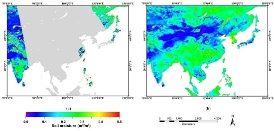
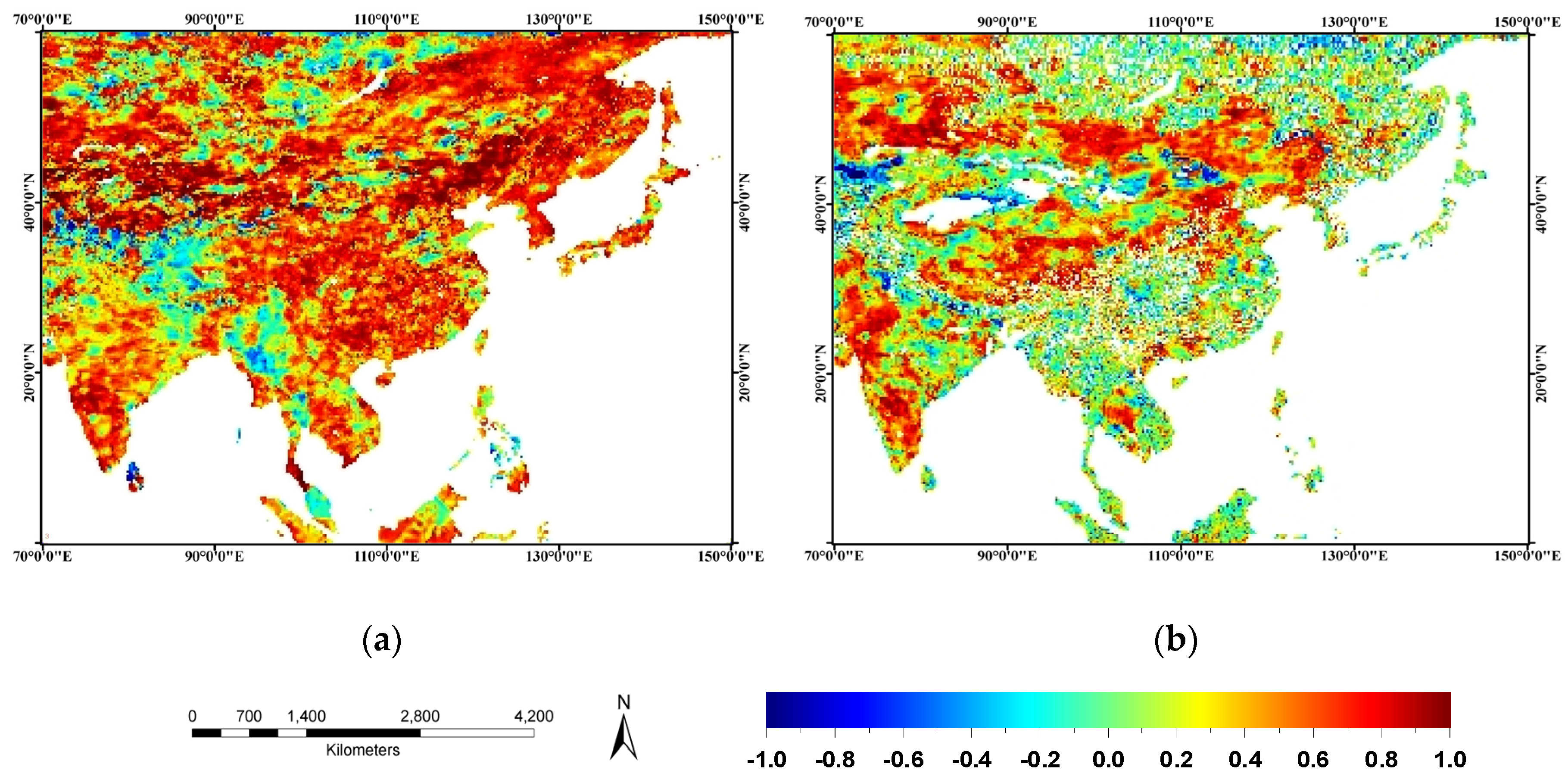
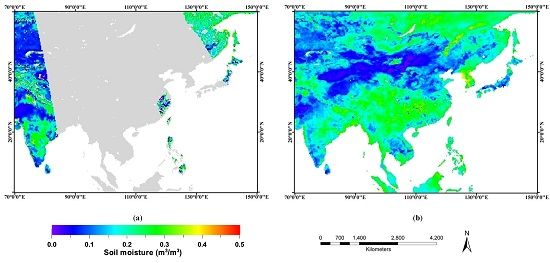
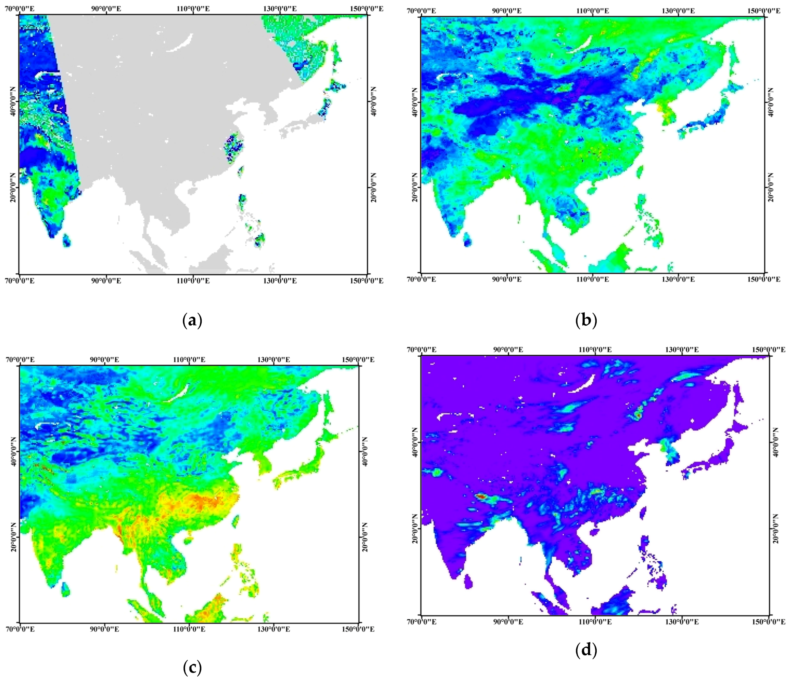
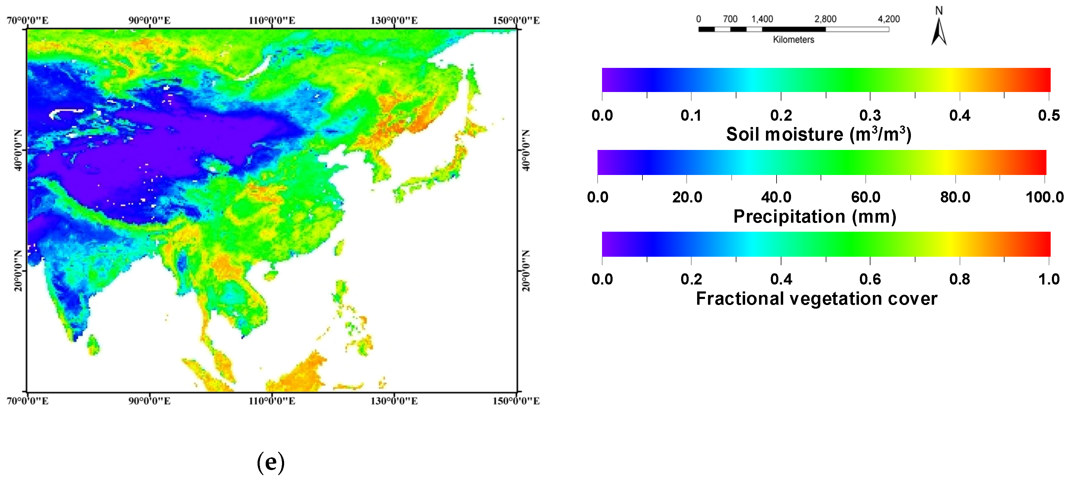
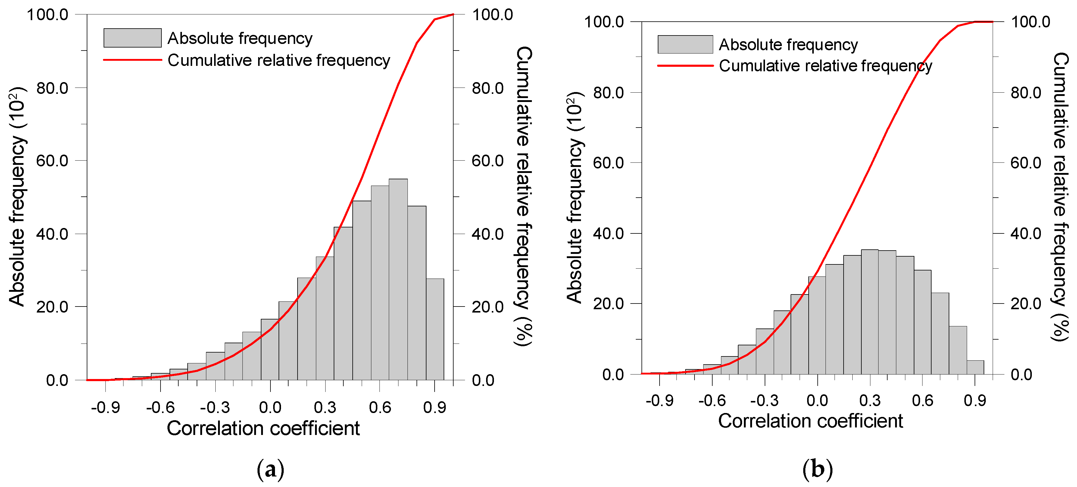
3.1. Comparison in Space

To investigate any discrepancies of the soil moisture data, as well to check the spatial distribution of missing data, maps of TCRM soil moisture for ascending orbits, reconstructed soil moisture, and soil moisture simulated by the GLDAS Noah model on Julian day 200, 2012 are shown in Figure 1. Areas masked in gray correspond to pixels where the soil moisture values are missing. Figure 1a shows a map of TCRM soil moisture for the ascending orbit on Julian day 200, 2012. Most soil moisture values for this day are missing. Soil moisture values are provided only in the eastern and western regions. Obviously, the missing soil moisture values are all filled in the reconstructed soil moisture data (Figure 1b). In other words, the reconstructed soil moisture product is spatially complete. The reconstructed soil moisture and the soil moisture simulated by the GLDAS Noah model are generally consistent in their spatial patterns. Higher soil moisture values are produced over the upper right and bottom areas of these images, whereas they are low over the upper left and middle areas of these images. However, discrepancies are evident in the relative magnitudes given by the soil moisture products. There is a relatively large discrepancy over the bottom areas of these images, where the TCRM and reconstructed soil moisture values are lower than the soil moisture values simulated by the GLDAS Noah model (Figure 1c). This discrepancy should be partly explained by the soil moisture values at different depths. The values simulated by the GLDAS Noah model correspond to the soil moisture in the surface 0–10 cm layer, while the TCRM and reconstructed values represent the soil moisture in the surface 0–5 cm layer. Figure 1d shows a map of precipitation on Julian day 200, 2012. The spatial distribution of the reconstructed soil moisture shows good consistency with the precipitation pattern. The reconstructed soil moisture values over areas with significant precipitation are clearly larger than those over other areas. For further analysis of the reconstructed soil moisture data, a map of fractional vegetation cover on Julian day 201, 2012 is shown in Figure 1e. The fractional vegetation cover is estimated on the basis of the measures of the transmittance of light through the canopy [50]. It is observed that the soil moisture values are generally larger over the area with higher land vegetation density.

Figure 1. (a) TCRM soil moisture for ascending orbits; (b) reconstructed soil moisture; (c) soil moisture simulated by the GLDAS Noah model; and (d) precipitation on Julian day 200, 2012; and (e) fractional vegetation cover on Julian day 201, 2012. All these maps are provided at the spatial resolution of 0.25°.

Figure 1. (a) TCRM soil moisture for ascending orbits; (b) reconstructed soil moisture; (c) soil moisture simulated by the GLDAS Noah model; and (d) precipitation on Julian day 200, 2012; and (e) fractional vegetation cover on Julian day 201, 2012. All these maps are provided at the spatial resolution of 0.25°.

Figure 2 displays the spatial variability of correlations between the reconstructed soil moisture data and those simulated by the GLDAS Noah model and of correlations between the TCRM soil moisture data and those simulated by the GLDAS Noah model for August 2012. For each pixel, the correlation was computed if there are 10 or more soil moisture values over the month. Note that the reconstructed soil moisture data in August have strong positive correlations with those simulated by the GLDAS Noah model over large areas of the region (Figure 2a), which indicates that the reconstructed soil moisture product provides reasonable soil moisture values for the pixels with missing data in the TCRM soil moisture product. However, the reconstructed soil moisture values in August have negative correlations with those simulated by the GLDAS Noah model over certain parts of the region, where the TCRM soil moisture product generally also has negative correlations with those simulated by the GLDAS Noah model (shown in Figure 2b).

Figure 2. Spatial variability of: (a) correlations between the reconstructed soil moisture data and those simulated by the GLDAS Noah model; and (b) correlations between TCRM soil moisture for the ascending orbit and those simulated by the GLDAS Noah model for August 2012. The maps are provided at the spatial resolution of 0.25°.

Figure 2. Spatial variability of: (a) correlations between the reconstructed soil moisture data and those simulated by the GLDAS Noah model; and (b) correlations between TCRM soil moisture for the ascending orbit and those simulated by the GLDAS Noah model for August 2012. The maps are provided at the spatial resolution of 0.25°.

Figure 3 shows frequency histograms of correlations between the reconstructed soil moisture data and those simulated by the GLDAS Noah model and of correlations between TCRM soil moisture data and those simulated by the GLDAS Noah model for August 2012. Pixels with positive correlations between the reconstructed soil moisture data and those simulated by the GLDAS Noah model constituted more than 90% of the total land pixels of the area under study, and pixels with relatively strong positive correlations of r > 0.5 also constituted more than 56% of the total land pixels (Figure 3a). However, the correlation between the TCRM soil moisture data and those simulated by the GLDAS Noah model is much lower. In this case, pixels with relatively strong positive correlations of r > 0.5 constituted only 30% of the total land pixels.

Figure 3. Frequency histograms of (a) correlations between the reconstructed soil moisture data and those simulated by the GLDAS Noah model; and (b) correlations between TCRM soil moisture values for the ascending orbit and those simulated by the GLDAS Noah model for August 2012.

Figure 3. Frequency histograms of (a) correlations between the reconstructed soil moisture data and those simulated by the GLDAS Noah model; and (b) correlations between TCRM soil moisture values for the ascending orbit and those simulated by the GLDAS Noah model for August 2012.

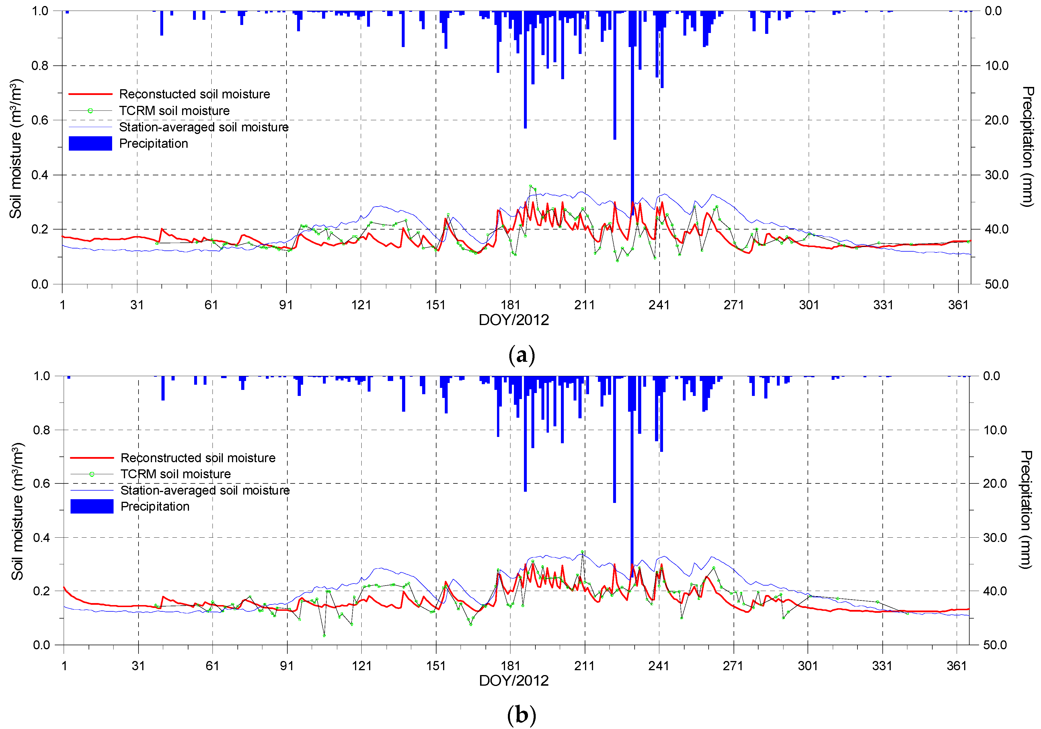
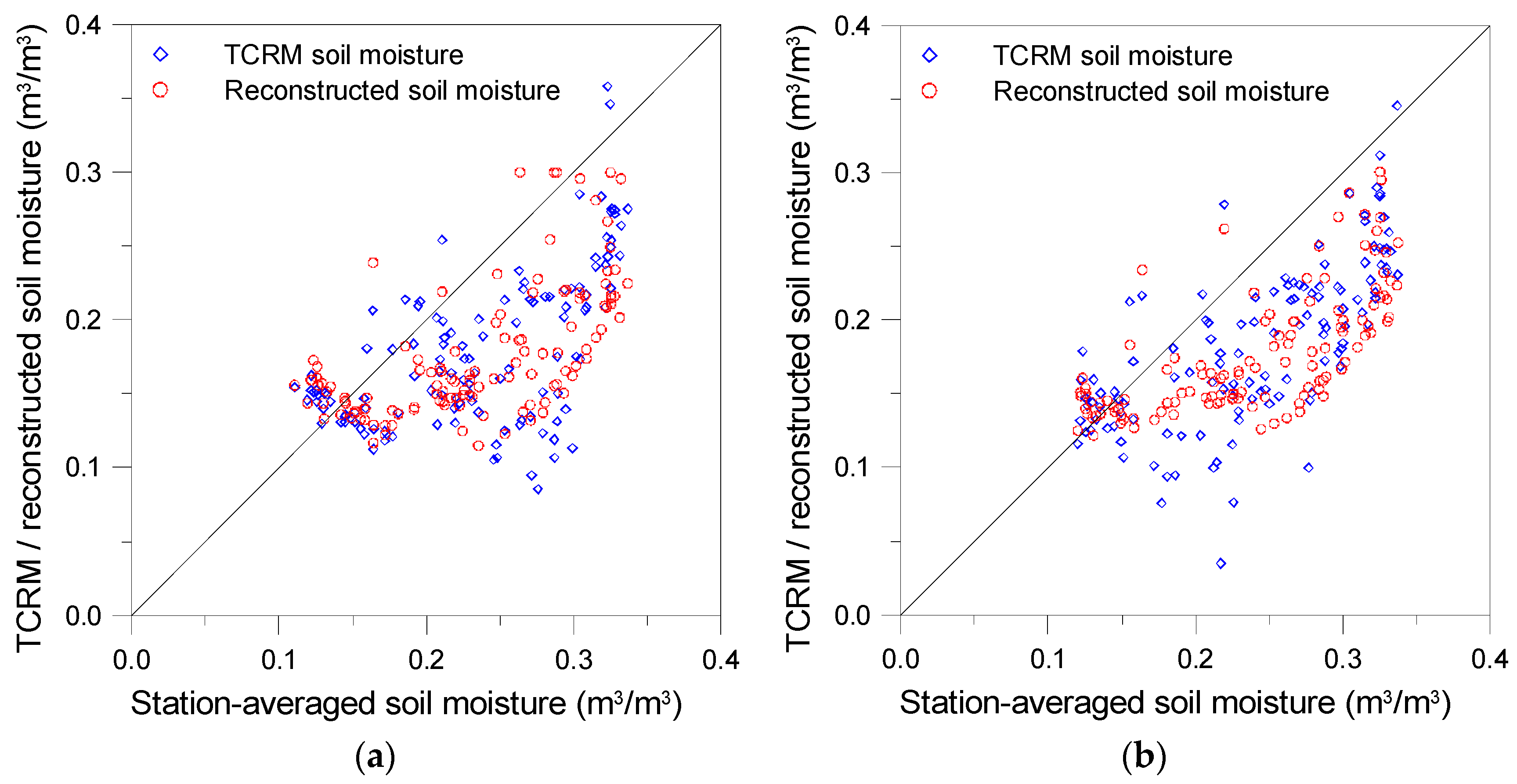
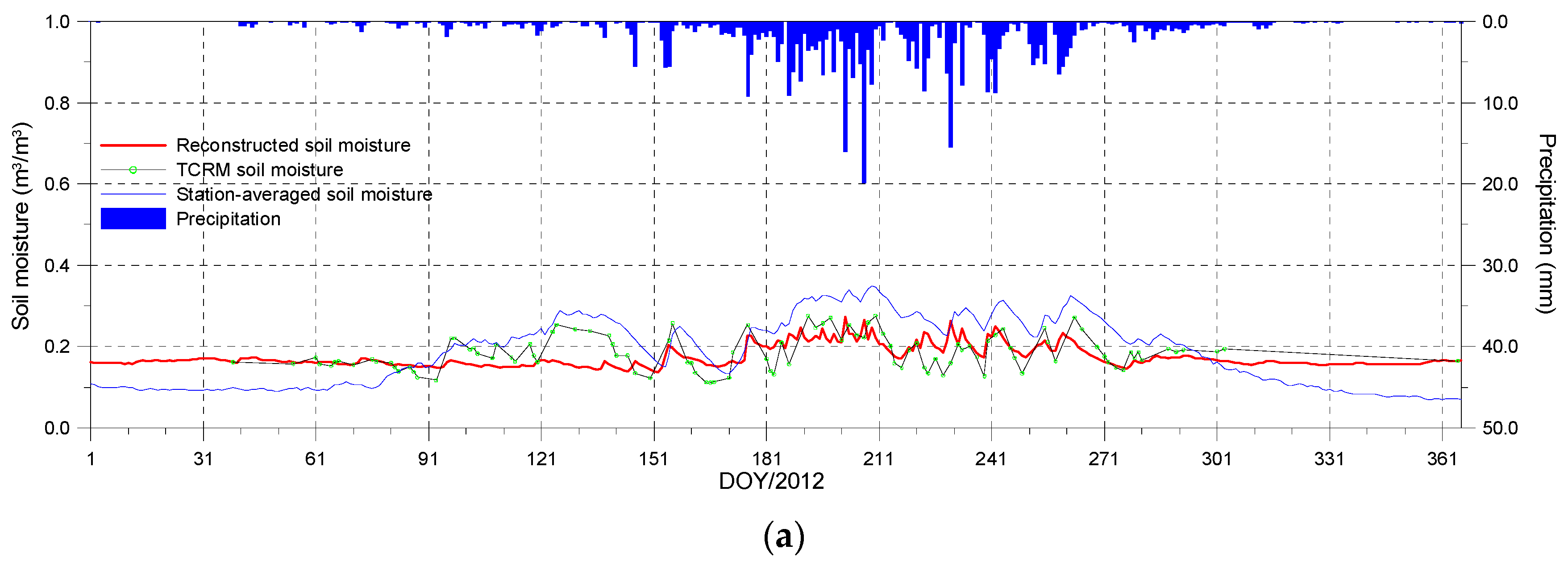
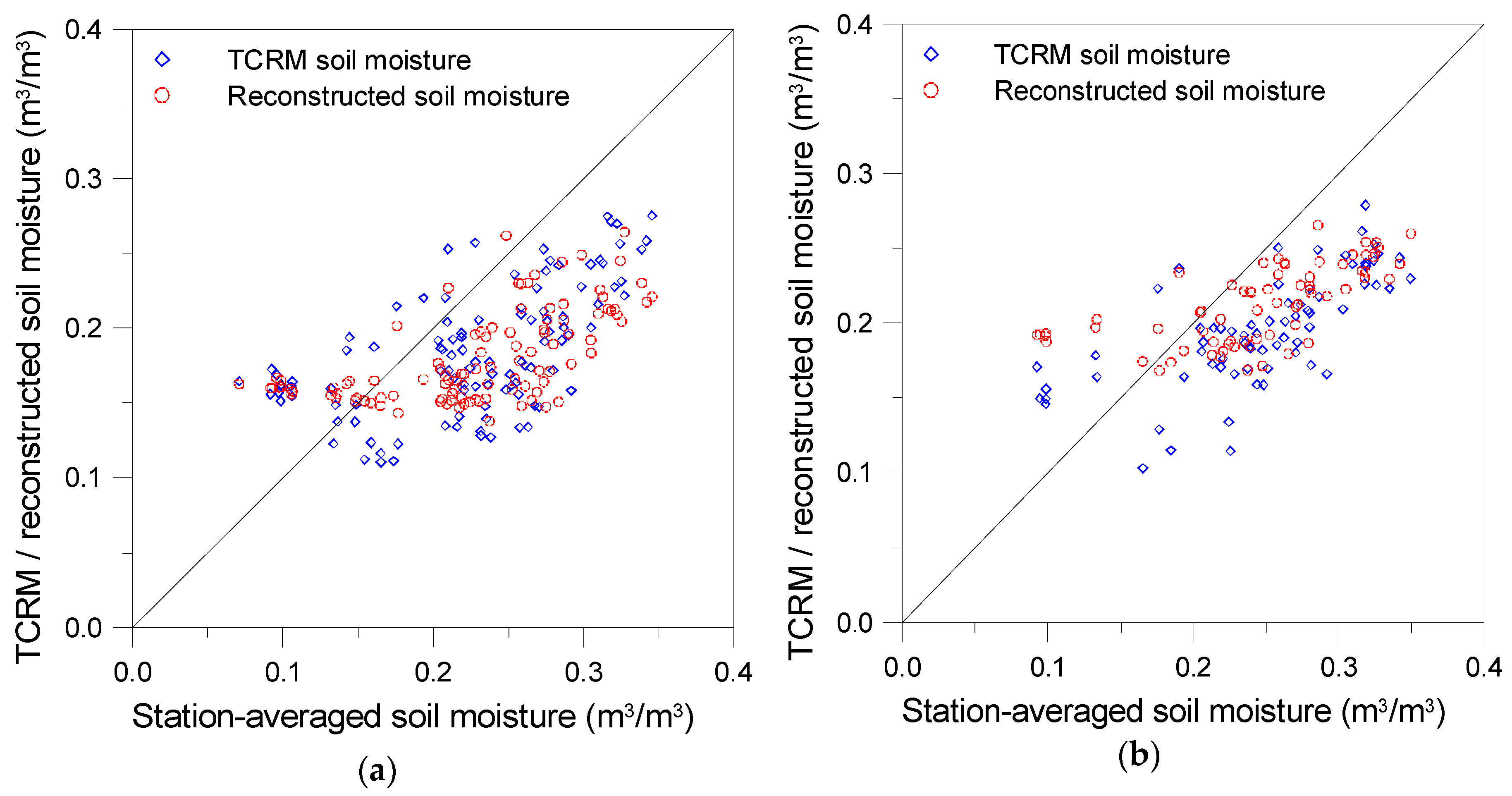
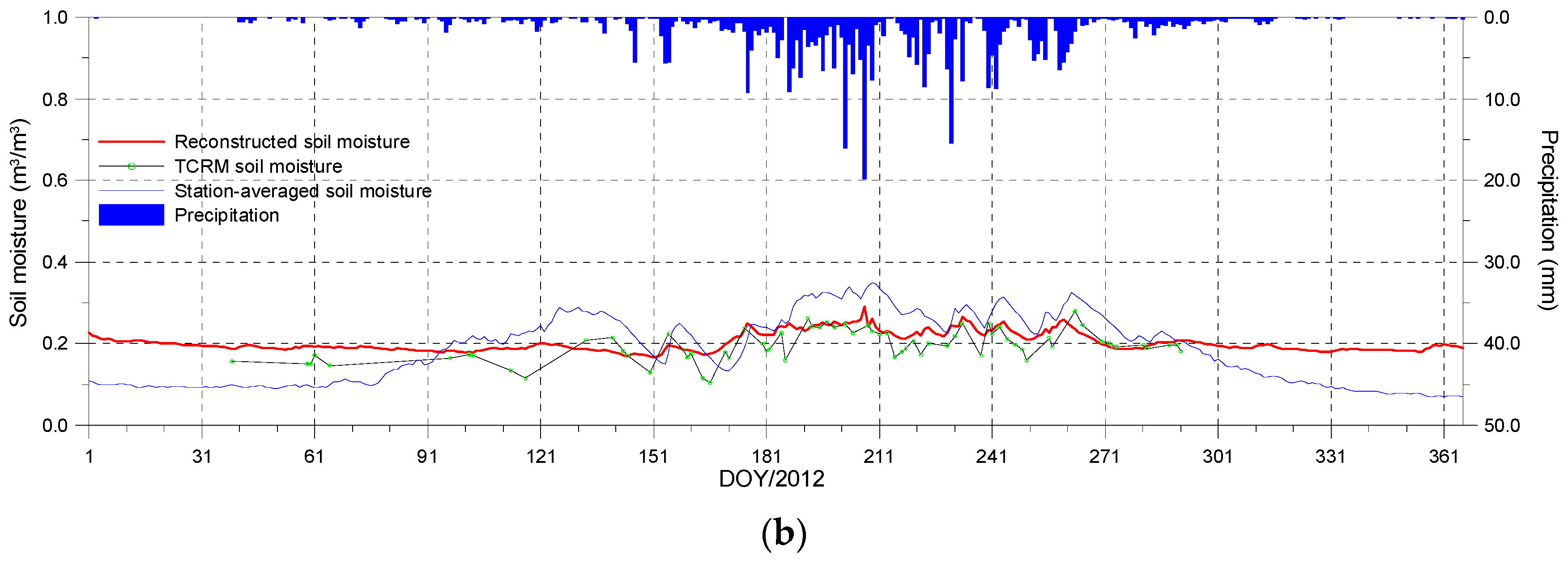
3.2. Comparison against Soil Moisture Measurements from Multi-Scale Networks

For the large network, time series of station-averaged soil moisture was calculated to represent the soil moisture values over the 1.0° × 1.0° region covered by the large network. The station-averaged soil moisture is defined as the arithmetic mean of the soil moisture measurements at the 38 stations of the large network. For time series comparison, average soil moisture profiles for the TCRM and reconstructed soil moisture data over the 1.0° × 1.0° region were calculated for the large network. The average soil moisture value over the 1.0° × 1.0° region was computed if more than 75% of the 0.25° pixels projected into the 1.0° × 1.0° region had soil moisture values. Otherwise, the average soil moisture value over the 1.0° × 1.0° region was set to fill value. Similarly, the station-averaged soil moisture and the average soil moisture of the TCRM and reconstructed soil moisture data for the medium network were also calculated. The average soil moisture profiles in 2012 were compared with time series of station-averaged soil moisture for the medium and large networks, respectively, to provide a qualitative assessment of seasonal variations and to analyze the precision of the TCRM and reconstructed soil moisture data in the time series.

Figure 4 displays time series of the TCRM and reconstructed soil moisture for descending and ascending orbits for the medium network in 2012. For convenience in comparison, time series of station-averaged soil moisture and precipitation for the medium network in 2012 is also shown in Figure 4. The reconstructed soil moisture is generally in good agreement with TCRM soil moisture. However, the reconstructed soil moisture has a more sensitive response to precipitation. The reconstructed soil moisture increases rapidly and then decreases slowly when there is significant precipitation.

Both TCRM and reconstructed soil moisture reflect seasonal changes in surface soil moisture and are generally in good agreement with station-averaged soil moisture for the medium network in terms of seasonal patterns. From Julian days 150 to 270, there is more precipitation, and soil moisture values can reach 0.3 or more and are higher than in other days. For the other days, soil moisture values are less than 0.2 as a result of less precipitation and frozen surface soil (0–5 cm). However, the station-averaged soil moisture values are larger than TCRM and reconstructed soil moisture during days 80–300, but lower than these soil moisture values at the beginning and end of the year.

Figure 4. Time series of TCRM and reconstructed soil moisture for (a) the ascending orbit; and (b) the descending orbit, with station-averaged soil moisture and precipitation for the medium networks in 2012. DOY (day of year) is Julian date.

Figure 4. Time series of TCRM and reconstructed soil moisture for (a) the ascending orbit; and (b) the descending orbit, with station-averaged soil moisture and precipitation for the medium networks in 2012. DOY (day of year) is Julian date.

Figure 5 presents a scatter plot of TCRM and reconstructed soil moisture against station-averaged soil moisture for the medium network in 2012. The error metrics are given in Table 1. Note that TCRM and reconstructed soil moisture for both ascending and descending orbits underestimate station-averaged soil moisture, as indicated by the negative bias values in Table 1. Most of the scatters below the 1:1 line belong to the unfrozen season. The TCRM data and reconstructed soil moisture data yield very close statistical values for R², RMSE, and Bias (Table 1). The statistical parameters in Table 1 also indicate that there is no obvious difference between the soil moisture values for ascending and descending orbits, a result which is in agreement with the findings of Jackson et al. [10].

Figure 5. Scatter plots of TCRM and reconstructed soil moisture for (a) the ascending orbit; and (b) the descending orbit against station-averaged soil moisture for the medium network in 2012.

Figure 5. Scatter plots of TCRM and reconstructed soil moisture for (a) the ascending orbit; and (b) the descending orbit against station-averaged soil moisture for the medium network in 2012.

Table 1. Soil moisture error metrics for the medium and large networks.

Area	Product	Ascending Orbit				Descending Orbit
		R2	RMSE	Bias	N	R2	RMSE	Bias	N
Medium network	TCRM	0.339	0.079	−0.056	124	0.479	0.075	−0.056	123
	DARM	0.378	0.078	−0.058	124	0.476	0.078	−0.061	123
Large network	TCRM	0.357	0.068	−0.042	107	0.473	0.068	−0.049	70
	DARM	0.373	0.072	−0.046	107	0.437	0.059	−0.032	70

DARM denotes the reconstructed soil moisture and N is the number of matched data pairs for each case.

Table 1. Soil moisture error metrics for the medium and large networks.

Area	Product	Ascending Orbit				Descending Orbit
		R2	RMSE	Bias	N	R2	RMSE	Bias	N
Medium network	TCRM	0.339	0.079	−0.056	124	0.479	0.075	−0.056	123
	DARM	0.378	0.078	−0.058	124	0.476	0.078	−0.061	123
Large network	TCRM	0.357	0.068	−0.042	107	0.473	0.068	−0.049	70
	DARM	0.373	0.072	−0.046	107	0.437	0.059	−0.032	70

DARM denotes the reconstructed soil moisture and N is the number of matched data pairs for each case.

Figure 6 shows the time series of TCRM and reconstructed soil moisture for descending and ascending orbits over the large network in 2012. For convenient comparison, the station-averaged soil moisture and precipitation over the large network in 2012 are also shown in Figure 6. Similarly to the results for the medium network, the TCRM and reconstructed soil moisture values reflected seasonal changes in surface soil moisture and showed similar seasonal changes to the station-averaged soil moisture in the large network. During the frozen season, there was very little precipitation. Time series of the reconstructed and station-averaged soil moisture also show very small variations.

Figure 6. Time series of TCRM and reconstructed soil moisture for (a) the ascending orbit; and (b) the descending orbit, with the station-averaged soil moisture and precipitation for the large network in 2012. The TCRM and reconstructed soil moisture values were aggregated to 1° spatial resolution. DOY (day of year) is Julian date.

Figure 6. Time series of TCRM and reconstructed soil moisture for (a) the ascending orbit; and (b) the descending orbit, with the station-averaged soil moisture and precipitation for the large network in 2012. The TCRM and reconstructed soil moisture values were aggregated to 1° spatial resolution. DOY (day of year) is Julian date.

Figure 7 shows scatter plots of TCRM and reconstructed soil moisture against station-averaged soil moisture for the large network in 2012. The error metrics are presented in Table 1. The negative bias values in Table 1 indicate that the TCRM and reconstructed soil moisture values for both ascending and descending orbits systematically underestimate station-averaged soil moisture. There is no obvious difference between the soil moisture for ascending and descending orbits. However, the statistical values of RMSE and Bias for the large network are slightly lower than those for the medium network.

Figure 7. Scatter plots of TCRM and reconstructed soil moisture for (a) the ascending orbit and (b) the descending orbit against station-averaged soil moisture for the large network in 2012.

Figure 7. Scatter plots of TCRM and reconstructed soil moisture for (a) the ascending orbit and (b) the descending orbit against station-averaged soil moisture for the large network in 2012.

4. Discussions

The method developed in this study has been used to reconstruct soil moisture time series from the TCRM soil moisture product. The results demonstrate that the method can efficiently reconstruct spatially and temporally complete soil moisture time series.

Nevertheless, the method relies solely on the TCRM soil moisture product to estimate the optimal values of the control variables. Therefore, the accuracy of the reconstructed soil moisture product largely depends on the accuracy of the TCRM soil moisture product. Comparison with station-averaged soil moisture for the medium and large networks indicates that the reconstructed soil moisture data have almost the same accuracy as TCRM soil moisture for ascending and descending orbits. In fact, there are very high RMSE (up to 0.08 m³/m³) and biases (about 0.06 m³/m³) for the TCRM and reconstructed soil moisture products. The high RMSE and biases between the satellite soil moisture and the station-averaged soil moisture are partly explained by measurement error of the station soil moisture. Yang et al. [49] showed that the sensors used to measure station soil moisture had an accuracy of ±2% volumetric water content. These high RMSE and biases should also be explained by the spatial representativeness of ground-based soil moisture measurements. For the large network, there are 38 stations located within an area of 1.0° × 1.0°, and the medium network consists of only 22 stations with a spatial extent of 0.3°. In this study, the station-averaged soil moisture values for the large and medium networks were calculated to evaluate the TCRM and reconstructed soil moisture products. More reliable strategies are needed to upscale the point-scale measurements to the grid-scale in the future. The retrieval algorithm assumption is the third factor that can lead to these high RMSE and biases in the TCRM and reconstructed soil moisture products. One potential solution to improve the accuracy of satellite soil moisture products is to estimate soil moisture from time series of brightness temperatures using a data assimilation method to integrate prior information from soil moisture models.

For the reconstructed soil moisture product, another source of uncertainty may come from the soil moisture model itself. In this study, empirical relationships were used to estimate the fraction of precipitation infiltrating into the soil, the evapotranspiration component and the drainage component due to deep percolation in the soil moisture model. Taking the potential evapotranspiration as an example, many methods have been developed to calculate the potential evapotranspiration. Among them, the Food and Agriculture Organisation (FAO) Penman-Monteith method [38] is considered to yield most accurate results [51]. However, the Penman-Monteith method is data-intensive [33]. In our further study, the Penman-Monteith method will be adopted to compute the potential evapotranspiration when the meteorological data are enough to support the use of the Penman-Monteith method.

5. Conclusions

Soil moisture products from satellite observations are not spatially and temporally complete due to track changes, radio-frequency interference, dense vegetation, and frozen soil. This research has developed a data assimilation algorithm to fill the gaps in the satellite soil moisture products and to generate spatially and temporally complete soil moisture data. Satellite soil moisture data covering one year were used to estimate the control variables of a soil moisture model. Soil moisture time series were then reconstructed by the soil moisture model using the optimal values of the control variables.

The method was used to reconstruct daily soil moisture time series from the soil moisture product derived from AMSR-E/MWRI/AMSR2 for ascending and descending orbits. The results show that the algorithm can efficiently reconstruct a spatially and temporally complete soil moisture time series. The reconstructed soil moisture data had strong positive correlations with those simulated by the GLDAS Noah model over large areas of the region. Comparisons with soil moisture measurements for the medium and large networks on the central Tibetan Plateau demonstrate that the reconstructed soil moisture data have almost the same accuracy as TCRM soil moisture for ascending and descending orbits.

The method developed in this study has been used only to reconstruct soil moisture data for 2012. In the near future, the authors will extend the methodology to long time series of soil moisture data from elsewhere in the world to satisfy the needs of different applications. Reconstruction of soil moisture data with a higher temporal resolution (e.g., one hour) will also be explored in a forthcoming study.

References

1. Kerr, Y.H.; Waldteufel, P.; Wigneron, J.P.; Martinuzzi, J.; Font, J.; Berger, M. Soil moisture retrieval from space: The Soil Moisture and Ocean Salinity (SMOS) mission. IEEE Trans. Geosci. Remote Sens. 2001, 39, 1729–1735. [Google Scholar] [CrossRef]
2. Bartalis, Z.; Wagner, W.; Naeimi, V.; Hasenauer, S.; Scipal, K.; Bonekamp, H.; Figa, J.; Anderson, C. Initial soil moisture retrievals from the METOPA Advanced Scatterometer (ASCAT). Geophys. Res. Lett. 2007, 34. [Google Scholar] [CrossRef]
3. Kawanishi, T.; Sezai, T.; Ito, Y.; Imaoka, K.; Takeshima, T.; Ishido, Y.; Shibata, A.; Miura, M.; Inahata, H.; Spencer, R.W. The Advanced Microwave Scanning Radiometer for the Earth Observing System (AMSR-E), NASDA’s contribution to the EOS for global energy and water cycle studies. IEEE Trans. Geosci. Remote Sens. 2003, 41, 184–194. [Google Scholar] [CrossRef]
4. Koike, T.; Nakamura, Y.; Kaihotsu, I.; Davva, G.; Matsuura, N.; Tamagawa, K.; Fujii, H. Development of an Advanced Microwave Scanning Radiometer (AMSR-E) algorithm of soil moisture and vegetation water content. Annu. J. Hydraul. Eng. Jpn. Soc. Civil Eng. 2004, 48, 217–222. [Google Scholar] [CrossRef]
5. Paris Anguela, T.; Zribi, M.; Habets, F.; Hasenauer, S.; Loumagne, C. Analysis of surface and root soil moisture dynamics with ERS scatterometer and the hydrometeorological model SAFRAN-ISBA-MODCOU at Grand Morin watershed (France). Hydrol. Earth Syst. Sci. 2008, 5, 1903–1926. [Google Scholar] [CrossRef]
6. Amri, R.; Zribi, M.; Lili-Chabaane, Z.; Wagner, W.; Hauesner, S. Analysis of ASCAT-C band scatterometer estimations derived over a semi-arid region. IEEE Trans. Geosci. Remote Sens. 2012, 50, 2630–2638. [Google Scholar] [CrossRef]
7. Wagner, W.; Scipal, K.; Pathe, C.; Gerten, D.; Lucht, W.; Rudolf, B. Evaluation of the agreement between the first global remotely sensed soil moisture data with model and precipitation data. J. Geophys. Res. 2003, 108. [Google Scholar] [CrossRef]
8. Rüdiger, C.; Calvet, J.; Gruhier, C.; Holmes, T.; de Jeu, R.; Wagner, W. An intercomparison of ERS-Scat and AMSR-E soil moisture observations with model simulations over France. J. Hydrometeorol. 2009, 10, 431–447. [Google Scholar] [CrossRef]
9. De Jeu, R.; Wagner, W.; Holmes, T.; Dolman, A.; van de Giesen, N.; Friesen, J. Global soil moisture patterns observed by space borne microwave radiometers and scatterometers. Surv. Geophys. 2008, 29, 399–420. [Google Scholar] [CrossRef]
10. Jackson, T.; Cosh, M.; Bindlish, R.; Starks, P.; Bosch, D.; Seyfried, M.; Goodrich, D.; Moran, S.; Du, J. Validation of advanced microwave scanning radiometer soil moisture products. IEEE Trans. Geosci. Remote Sens. 2010, 48, 4256–4272. [Google Scholar] [CrossRef]
11. Jackson, T.; Bindlish, R.; Cosh, M.; Zhao, T.; Starks, P.; Bosch, D.; Seyfried, M.; Moran, M.; Goodrich, D.; Kerr, Y.; et al. Validation of Soil Moisture and Ocean Salinity (SMOS) soil moisture over watershed networks in the U.S. IEEE Trans. Geosci. Remote Sens. 2012, 50, 1530–1543. [Google Scholar] [CrossRef] [Green Version]
12. Bitar, A.; Leroux, D.; Kerr, Y.; Merlin, O.; Richaume, P.; Sahoo, A.; Wood, E. Evaluation of SMOS soil moisture products over continental U.S. using the SCAN/SNOTEL network. IEEE Trans. Geosci. Remote Sens. 2012, 50, 1572–1586. [Google Scholar] [CrossRef] [Green Version]
13. Brocca, L.; Hasenauerb, S.; Lacavac, T.; Melonea, F.; Moramarcoa, T.; Wagnerb, W.; Dorigob, W.; Matgend, P.; Martínez-Fernándeze, J.; Llorensf, P.; et al. Soil moisture estimation through ASCAT and AMSR-E sensors: An intercomparison and validation study across Europe. Remote Sens. Environ. 2011, 115, 3390–3408. [Google Scholar] [CrossRef]
14. Draper, C.; Walker, J.; Steinle, P.; de Jeu, R.; Holmes, T. An evaluation of AMSR-E derived soil moisture over Australia. Remote Sens. Environ. 2009, 113, 703–710. [Google Scholar] [CrossRef]
15. Su, Z.; Wen, J.; Dente, L.; van der Velde, R.; Wang, L.; Ma, Y.; Yang, K.; Hu, Z. The Tibetan Plateau observatory of plateau scale soil moisture and soil temperature (Tibet-Obs) for quantifying uncertainties in coarse resolution satellite and model products. Hydrol. Earth Syst. Sci. 2011, 15, 2303–2316. [Google Scholar] [CrossRef]
16. Wang, G.; Garcia, D.; Liu, Y.; Jeu, R.D.; Dolman, A.J. A three-dimensional gap filling method for large geophysical datasets: Application to global satellite soil moisture observations. Environ. Model. Softw. 2012, 30, 139–142. [Google Scholar] [CrossRef]
17. Varella, H.; Guérif, M.; Buis, S. Global sensitivity analysis measures the quality of parameter estimation: The case of soil parameters and a crop model. Environ. Model. Softw. 2010, 25, 310–319. [Google Scholar] [CrossRef]
18. Viovy, N.; Arino, O.; Belward, A.S. The Best Index Slope Extraction (BISE)—A method for reducing noise in NDVI time-series. Int. J. Remote Sens. 1992, 13, 1585–1590. [Google Scholar] [CrossRef]
19. Hermance, J.F. Stabilizing high-order, non-classical harmonic analysis of NDVI data for average annual models by damping model roughness. Int. J. Remote Sens. 2007, 28, 2801–2819. [Google Scholar] [CrossRef]
20. Julien, Y.; Sobrino, J.A.; Verhoef, W. Changes in land surface temperatures and NDVI values over Europe between 1982 and 1999. Remote Sens. Environ. 2006, 103, 43–55. [Google Scholar] [CrossRef]
21. Xiao, Z.; Liang, S.; Wang, T.; Liu, Q. Reconstruction of satellite-retrieved land-surface reflectance based on temporally-continuous vegetation indices. Remote Sens. 2015, 7, 9844–9864. [Google Scholar] [CrossRef]
22. Jönsson, P.; Eklundh, L. Seasonality extraction by function fitting to time—Series of satellite sensor data. IEEE Trans. Geosci. Remote Sens. 2002, 40, 1824–1832. [Google Scholar] [CrossRef]
23. Sellers, P.; Tucker, C.; Collatz, G.; Los, S.; Justice, C.; Dazlich, D.; Randall, D. A global 1 by 1 NDVI data set for climate studies. Part 2: The generation of global fields of terrestrial biophysical parameters from the NDVI. Int. J. Remote Sens. 1994, 15, 3519–3546. [Google Scholar] [CrossRef]
24. Jönsson, P.; Eklundh, L. TIMESAT—A program for analyzing time-series of satellite sensor data. Comput. Geosci. 2004, 30, 833–845. [Google Scholar] [CrossRef]
25. Roerink, G.J.; Menenti, M.; Verhoef, W. Reconstructing cloud free NDVI composites using Fourier analysis of time series. Int. J. Remote Sens. 2000, 21, 1911–1917. [Google Scholar] [CrossRef]
26. Fang, H.; Liang, S.; Townshend, J.; Dickinson, R. Spatially and temporally continuous LAI data sets based on an integrated filtering method: Examples from North America. Remote Sens. Environ. 2008, 112, 75–93. [Google Scholar] [CrossRef]
27. Moody, E.G.; King, M.D.; Platnick, S.; Schaaf, C.B.; Gao, F. Spatially complete global spectral surface albedos: Value-add datasets derived from Terra MODIS land products. IEEE Trans. Geosci. Remote Sens. 2005, 43, 144–157. [Google Scholar] [CrossRef]
28. Rodell, M.; Houser, P.R.; Jambor, U.; Gottschalck, J.; Mitchell, K.; Meng, C-J.; Arsenault, K.; Cosgrove, B.; Radakovich, J.; Bosilovich, M.; et al. The global land data assimilation system. Bull. Am. Meteor. Soc. 2004, 85, 381–394. [Google Scholar] [CrossRef]
29. Chen, Y.; Yang, K.; Qin, J.; Zhao, L.; Tang, W.; Han, M. Evaluation of AMSR-E retrievals and GLDAS simulations against observations of a soil moisture network on the central Tibetan plateau. J. Geophys. Res. Atmos. 2013, 118, 4466–4475. [Google Scholar] [CrossRef]
30. Hain, C.R.; Crow, W.T.; Anderson, M.C.; Mecikalski, J.R. An ensemble Kalman filter dual assimilation of thermal infrared and microwave satellite observations of soil moisture into the Noah land surface model. Water Resour. Res. 2012, 48. [Google Scholar] [CrossRef]
31. Crow, W.T.; Wood, E.F. The assimilation of remotely sensed soil brightness temperature imagery into a land surface model using ensemble Kalman filtering: A case study based on ESTAR measurements during SGP97. Adv. Water Resour. 2003, 26, 137–149. [Google Scholar] [CrossRef]
32. Reichle, R.H.; Koster, R.D. Global assimilation of satellite surface soilmoisture retrievals into the NASA catchment land surface model. Geophys. Res. Lett. 2005, 32. [Google Scholar] [CrossRef]
33. Venkatesh, B.; Nandagiri, L.; Purandara, B.K.; Reddy, V.B. Modelling soil moisture under different land covers in a sub-humid environment of Western Ghats. India J. Earth Syst. Sci. 2011, 120, 387–398. [Google Scholar] [CrossRef]
34. Brocca, L.; Melone, F.; Moramarco, T. On the estimation of antecedent wetness conditions in rainfall-runoff modelling. Hydrol. Process. 2008, 22, 629–642. [Google Scholar] [CrossRef]
35. Turc, L. Evaluation des besoins en eau d’irrigation, évapotranspiration potentielle. Ann. Agron. 1961, 12, 13–49. [Google Scholar]
36. Hargreaves, G.H.; Samani, Z.A. Estimating potential evapotranspiration. J. Irrig. Drain. E-Asce 1982, 108, 225–230. [Google Scholar]
37. Hargreaves, G.H.; Samani, Z.A. Reference crop evapotranspiration from temperature. Appl. Eng. Agric. 1985, 1, 96–99. [Google Scholar] [CrossRef]
38. Allen, R.; Pereira, L.S.; Raes, D.; Smith, M. Crop evapotranspiration. In Guidelines for Computing Crop Water Requirements; Irrigation Drainage Paper No.56; Food and Agriculture Organization of the United Nations: Rome, Italy, 1998. [Google Scholar]
39. Duan, Q.; Sorooshian, S.; Gupta, V.K. Effective and efficient global optimization for conceptual rainfall-runoff models. Water Resour. Res. 1992, 28, 1015–1031. [Google Scholar] [CrossRef]
40. Shi, C.; Xie, Z.; Qian, H.; Liang, M.; Yang, X. China land soil moisture EnKF data assimilation based on satellite remote sensing data. Sci. China Earth Sci. 2011, 54, 1430–1440. [Google Scholar] [CrossRef]
41. Sheng, P.; Mao, J.; Li, J.; Zhang, A.; Sang, J.; Pan, N. Atmospheric Physics; Peking University Press: Beijing, China, 2003. [Google Scholar]
42. Shi, J.; Jiang, L.; Zhang, L.; Chen, K.; Wigneron, J.P.; Chanzy, A. A parameterized multifrequency-polarization surface emission model. IEEE Trans. Geosci. Remote Sens. 2005, 43, 2831–2841. [Google Scholar]
43. Liu, Q.; Du, J.; Shi, J.; Jiang, L.M. Analysis of spatial distribution and multi-year trend of the remotely sensed soil moisture on the Tibetan Plateau. Sci. China Earth Sci. 2013, 56, 2173–2185. [Google Scholar] [CrossRef]
44. Du, J.; Kimball, J.S.; Shi, J.; Jones, L.A.; Wu, S.; Sun, R.; Yang, H. Inter-calibration of satellite passive microwave land observations from AMSR-E and AMSR2 using overlapping FY3B-MWRI sensor measurements. Remote Sens. 2014, 6, 8594–8616. [Google Scholar] [CrossRef]
45. Jiang, L.; Lu, L.; Qi, Y.; Du, J.; Tao, J. Comparison of satellite soil moisture products with field observations and model simulation in the Tibetan Plateau. Remote Sens. Environ. 2015, submitted. [Google Scholar]
46. Njoku, E.; Chan, S. Vegetation and surface roughness effects on AMSR-E land observations. Remote Sens. Environ. 2006, 100, 190–199. [Google Scholar] [CrossRef]
47. Owe, M.; de Jeu, R.; Holmes, T. Multisensor historical climatology of satellite-derived global land surface moisture. J. Geophys. Res. 2008, 113, F01002. [Google Scholar] [CrossRef]
48. Goddard Earth Sciences Data and Information Services Center. Available online: http://disc.sci.gsfc.nasa.gov/hydrology/data-holdings (accessed on 19 September 2015).
49. Yang, K.; Qin, J.; Zhao, L.; Chen, Y.; Tang, W.; Han, M.; Zhu, L.; Chen, Z.Q.; Lv, N.; Ding, B.H.; et al. A multi-scale soil moisture and freeze-thaw monitoring network on the Third Pole. Bull. Am. Meteorol. Soc. 2013, 94, 1907–1916. [Google Scholar] [CrossRef]
50. Xiao, Z.; Wang, T.; Liang, S.; Sun, R. Estimating the fractional vegetation cover from GLASS leaf area index product. Remote Sens. 2015. under review. [Google Scholar] [CrossRef]
51. Nandagiri, L.; Kovoor, G. Performance evaluation of reference evapotranspiration equations across a range of Indian climates. J. Irrig. Drain. Eng. 2006, 132, 238–249. [Google Scholar] [CrossRef]