
Scaling up Ecological Measurements of Coral Reefs Using Semi-Automated Field Image Collection and Analysis

 ,
,  and
and
Abstract
:
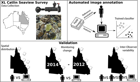
1. Introduction
2. Material and Methods
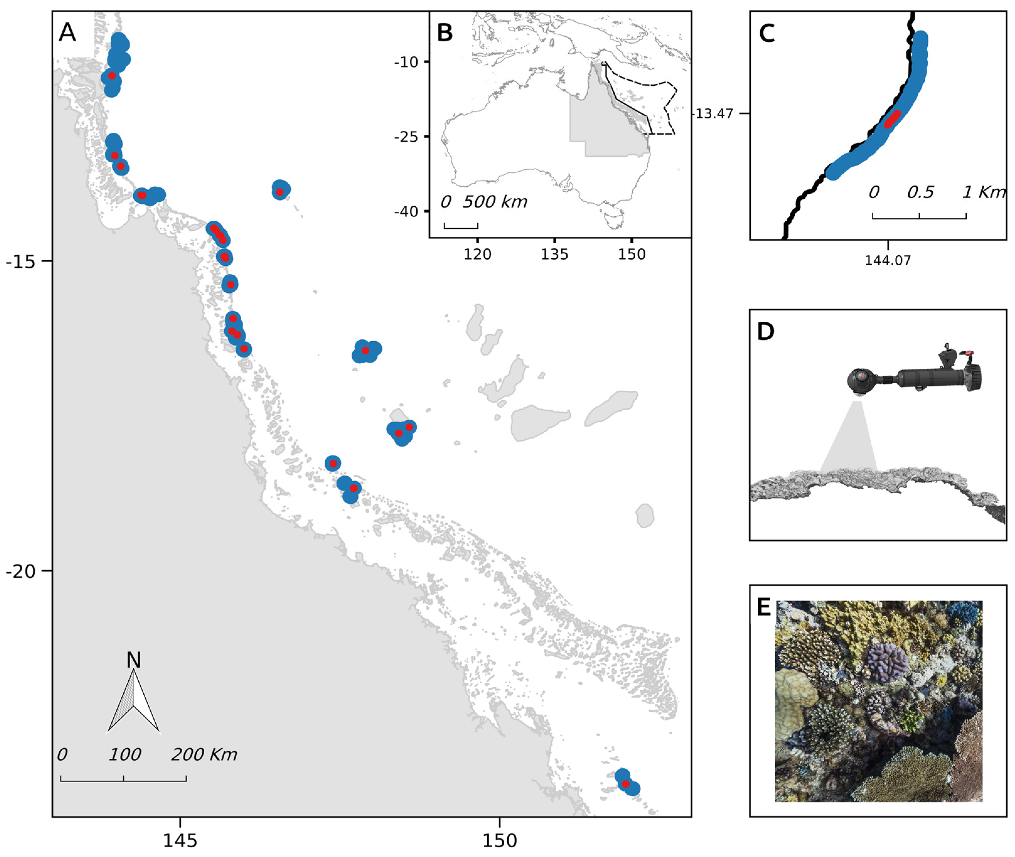
2.1. Study Site

2.2. Field Image Collection
2.3. Image Analysis
2.3.1. Label Set for Benthic Categories

| Group | Short Name | Taxonomic Description | Overall Functional Attributes | Ref. |
|---|---|---|---|---|
| Hard Coral | Acr. branching | Family Acroporidae, branching morphology (excluding hispidose type branching). | Major reef framework builders. Competitive life-history strategy: fast-growing species, spawning reproduction, high susceptibility to thermal stress (bleaching) and wave action. Provide habitat to a range of other reef-dwelling species. | [41,42,43,44,45,46,47] |
| Acr. hispidose | Family Acroporidae, hispidose morphology | Competitive life-history strategy: fast-growing species, spawning reproduction, high susceptibility to thermal stress (bleaching) and wave action. | [44,45,46,47] | |
| Acr. other | Other corals from the family Acroporidae (e.g., Isopora) | Brooding reproduction, severe/high susceptibility to thermal stress, and low/moderate susceptibility to wave action. | [44,45,47,48] | |
| Acr. encrusting | Family Acroporidae, plate and encrusting morphologies | Major reef framework builders. Competitive and generalist life-history strategies: fast/moderate growth rates, spawning reproduction, high/severe susceptibility to thermal stress, moderate to low susceptibility to wave action. | [43,44,45,46,48] | |
| Acr. Tabular | Family Acroporidae, table, corymbose and digitate morphologies | Major reef framework builders. Competitive life-history strategy: fast-growing species, spawning reproduction, high/severe susceptibility to thermal stress (bleaching), and high to low susceptibility to wave action. High to moderate susceptibility to disease outbreaks. Largely contribute to reef structural complexity. | [43,44,45,46,49,50] | |
| Massive meandroid | Families Favidae and Mussidae, massive and meandroid morphologies | Major reef framework builders. Stress-tolerant life history: slow-growing species, spawning reproduction, moderate susceptibility to thermal stress, and low susceptibility to wave action. | [43,44,45,46,48] | |
| Other corals | Other hard coral including all other groups not represented by the other coral categories of this label set. | Mixed attributes. Low/moderate susceptibility to thermal stress. | [51] | |
| Pocillopora | Family Pocilloporidae | Reef framework builders. Competitive and weedy life-history strategies: early colonisers in reef succession trajectories, fast-growing species, brooding reproduction, highly susceptible to thermal stress, but moderate resistant to wave action. High prevalence of coral diseases. | [43,44,45,46,48,51,52] | |
| Por. branching | Family Poritidae, branching morphology | Weedy life-history strategy: spawning reproduction, high/moderate susceptibility to thermal stress. | [45,46,53] | |
| Por. encrusting | Family Poritidae, encrusting morphology | Brooding reproduction. Low/moderate susceptible to thermal stress. | [51,54] | |
| Por. massive | Family Poritidae, massive morphology | Major reef framework builders. Stress-tolerant life history: slow-growing species, spawning reproduction, low/moderate susceptibility to thermal stress, and low susceptibility to wave action. | [43,44,45,46,48] | |
| Algae | CCA | Crustose Coralline Algae | Major reef framework builders and cementers. Provide key contribution to coral reef primary production. Facilitation of coral recruitment. | [55,56,57,58] |
| Macroalgae | Macroalgae. All genera. | Key contribution to coral reef primary production. Provide food source and habitat to a range of other reef dwelling species. Critical role during phase shifts. | [59,60,61,62] | |
| Turf | Multi-specific algal assemblage of 1 cm or less in height | Provide key contribution to coral reef primary production. Nitrogen fixation. Provide food source and habitat to a range of other reef dwelling species. | [63,64,65,66] | |
| Others | Sand | Unconsolidated reef sediment | Not applicable (N/A) | N/A |
| Other Invert. | Other sessile invertebrates | Mixed attributes. | N/A | |
| Soft Coral | Alc. Soft coral | Soft coral, family Alcyoniidae, genera Lobophytum and Sarcophytum. | An important contributor to reef’s structural complexity and biodiversity, providing habitat to a range of other reef-dwelling species. Slow-growing and suspension feeders. Spawning and asexual propagation. Deplete large amounts of suspended particulate matter. | [67,68,69,70] |
| Gorg. Soft coral | Sea fans and plumes | Provide habitat to a range of other reef-dwelling species. Spawning and brooding reproduction. Suspension feeders. | [67,68,69] | |
| Other Soft coral | Other Soft corals | Mixed attributes. | N/A |
2.3.2. Point Annotations
| Description | # Images | # Points·Image−1 | # Sites |
|---|---|---|---|
| Training of automated annotator | 1237 | 100 | N/A |
| Spatial error | 1042 | 40 | 41 |
| Temporal error | 335 | 40 | 7 |
| Inter-observer variability | 124 | 40 | 5 |
2.3.3. Automated Estimation of Benthic Composition
2.4. Validation of Automated Analysis of Field Imagery
2.4.1. Evaluation Sites
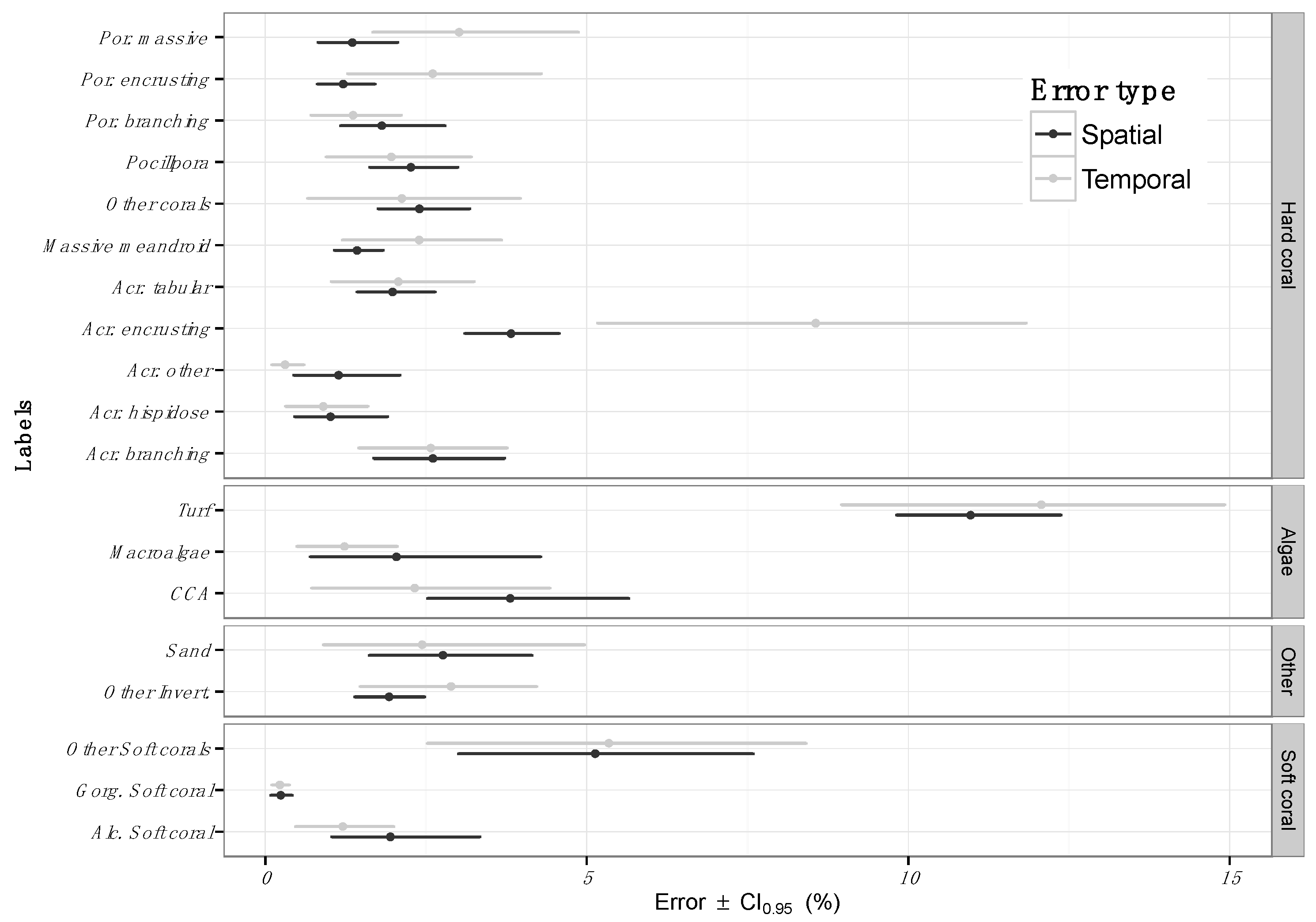
2.4.2. Estimating Error across Space
2.4.3. Estimating Error in Detecting Change over Time
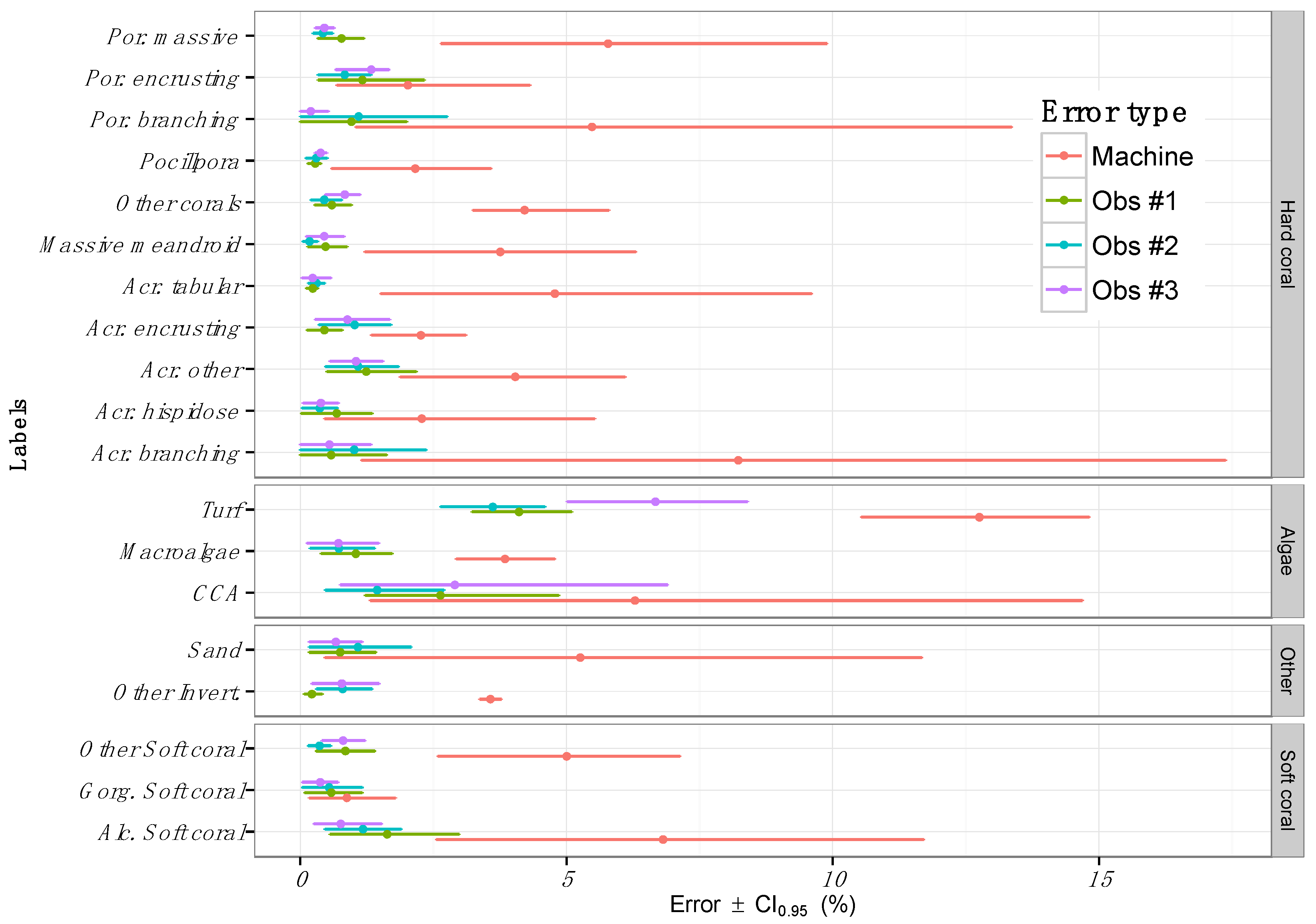
2.4.4. Inter-Observer Variability
3. Results
3.1. Estimating Error across Space

3.2. Estimating Error in Detecting Change over Time
3.3. Inter-Observer Variability

4. Discussion
4.1. Error across Space
4.2. Error in Detecting Change over Time
4.3. Sources of Error
4.4. Future Directions
5. Conclusions
Acknowledgments
Author Contributions
Conflicts of Interest
Appendix
Defining Sampling Units by Structure Functions

References
- Hughes, T.P.; Graham, N.A.J.; Jackson, J.B.C.; Mumby, P.J.; Steneck, R.S. Rising to the challenge of sustaining coral reef resilience. Trends Ecol. Evol. 2010, 25, 633–642. [Google Scholar] [CrossRef] [PubMed]
- Knowlton, N.; Jackson, J.B.C. Shifting baselines, local impacts, and global change on coral reefs. PLoS Biol. 2008, 6. [Google Scholar] [CrossRef] [PubMed]
- Fabricius, K.E.; Okaji, K.; De’ath, G. Three lines of evidence to link outbreaks of the crown-of-thorns seastar acanthaster planci to the release of larval food limitation. Coral Reefs 2010, 29, 593–605. [Google Scholar] [CrossRef]
- Baker, A.C.; Glynn, P.W.; Riegl, B. Climate change and coral reef bleaching: An ecological assessment of long-term impacts, recovery trends and future outlook. Estuar Coast. Shelf Sci. 2008, 80, 435–471. [Google Scholar] [CrossRef]
- Hoegh-Guldberg, O. Climate change, coral bleaching and the future of the world’s coral reefs. Mar. Freshw. Res. 1999, 50, 839–866. [Google Scholar] [CrossRef]
- De’ath, G.; Fabricius, K.E.; Sweatman, H.; Puotinen, M. The 27-year decline of coral cover on the great barrier reef and its causes. Proc. Natl. Acad. Sci. USA 2012, 109, 17995–17999. [Google Scholar] [CrossRef] [PubMed]
- Brodie, J.; Fabricius, K.; De’ath, G.; Okaji, K. Are increased nutrient inputs responsible for more outbreaks of crown-of-thorns starfish? An appraisal of the evidence. Mar. Pollut. Bull. 2005, 51, 266–278. [Google Scholar] [CrossRef] [PubMed]
- Hoegh-Guldberg, O.; Cai, R.; Poloczanska, E.S.; Brewer, P.G.; Sundby, S.; Hilmi, K.; Fabry, V.J.; Jung, S. The ocean. In Climate Change 2014: Impacts, Adaptation, and Vulnerability. Part B: Regional Aspects; Barros, V.R., Field, C.B., Dokken, D.J., Mastrandrea, M.D., Mach, K.J., Bilir, T.E., Chatterjee, M., Ebi, K.L., Estrada, Y.O., Genova, R.C., et al., Eds.; Cambridge University Press: Cambridge, UK, 2014; pp. 1655–1734. [Google Scholar]
- Gattuso, J.P.; Magnan, A.; Billé, R.; Cheung, W.; Howes, E.; Joos, F.; Allemand, D.; Bopp, L.; Cooley, S.; Eakin, C. Contrasting futures for ocean and society from different anthropogenic CO2 emissions scenarios. Science 2015, 349. [Google Scholar] [CrossRef] [PubMed] [Green Version]
- Gardner, T.A.; Cote, I.M.; Gill, J.A.; Grant, A.; Watkinson, A.R. Long-term region-wide declines in caribbean corals. Science 2003, 301, 958–960. [Google Scholar] [CrossRef] [PubMed]
- Schutte, V.G.; Selig, E.R.; Bruno, J.F. Regional spatio-temporal trends in caribbean coral reef benthic communities. Mar. Ecol. Prog. Ser. 2010, 402, 115–122. [Google Scholar] [CrossRef]
- Hughes, T.; Baird, A.; Dinsdale, E.; Harriott, V.; Moltschaniwskyj, N.; Pratchett, M.; Tanner, J.; Willis, B. Detecting regional variation using meta-analysis and large-scale sampling: Latitudinal patterns in recruitment. Ecology 2002, 83, 436–451. [Google Scholar] [CrossRef]
- Parmesan, C.; Yohe, G. A globally coherent fingerprint of climate change impacts across natural systems. Nature 2003, 421, 37–42. [Google Scholar] [CrossRef] [PubMed]
- Côté, I.; Gill, J.; Gardner, T.; Watkinson, A. Measuring coral reef decline through meta-analyses. Philos. Trans. R. Soc. B Biol. Sci. 2005, 360, 385–395. [Google Scholar] [CrossRef] [PubMed]
- Scopélitis, J.; Andréfouët, S.; Largouët, C. Modelling coral reef habitat trajectories: Evaluation of an integrated timed automata and remote sensing approach. Ecol. Model. 2007, 205, 59–80. [Google Scholar] [CrossRef]
- Mumby, P.J.; Hastings, A.; Edwards, H.J. Thresholds and the resilience of caribbean coral reefs. Nature 2007, 450, 98–101. [Google Scholar] [CrossRef] [PubMed]
- Roelfsema, C.; Phinn, S. Integrating field data with high spatial resolution multispectral satellite imagery for calibration and validation of coral reef benthic community maps. J. Appl. Remote Sens. 2010, 4. [Google Scholar] [CrossRef] [Green Version]
- Mumby, P.J.; Skirving, W.; Strong, A.E.; Hardy, J.T.; LeDrew, E.F.; Hochberg, E.J.; Stumpf, R.P.; David, L.T. Remote sensing of coral reefs and their physical environment. Mar. Pollut. Bull. 2004, 48, 219–228. [Google Scholar] [CrossRef] [PubMed]
- Hedley, J.D.; Roelfsema, C.M.; Phinn, S.R.; Mumby, P.J. Environmental and sensor limitations in optical remote sensing of coral reefs: Implications for monitoring and sensor design. Remote Sens. 2012, 4, 271–302. [Google Scholar] [CrossRef]
- Wooldridge, S.; Done, T. Learning to predict large-scale coral bleaching from past events: A bayesian approach using remotely sensed data, in-situ data, and environmental proxies. Coral Reefs 2004, 23, 96–108. [Google Scholar]
- Roelfsema, C.; Phinn, S.; Udy, N.; Maxwell, P. An integrated field and remote sensing approach for mapping seagrass cover, moreton bay, australia. J. Spat. Sci. 2009, 54, 45–62. [Google Scholar] [CrossRef]
- Carleton, J.H.; Done, T.J. Quantitative video sampling of coral reef benthos: Large-scale application. Coral Reefs 1995, 14, 35–46. [Google Scholar] [CrossRef]
- Ninio, R.; Delean, J.; Osborne, K.; Sweatman, H. Estimating cover of benthic organisms from underwater video images: Variability associated with multiple observers. Mar. Ecol. Prog. Ser. 2003, 265, 107–116. [Google Scholar] [CrossRef]
- González-Rivero, M.; Bongaerts, P.; Beijbom, O.; Pizarro, O.; Friedman, A.; Rodriguez-Ramirez, A.; Upcroft, B.; Laffoley, D.; Kline, D.; Bailhache, C.; et al. The Catlin Seaview Survey—Kilometre-scale seascape assessment, and monitoring of coral reef ecosystems. Aquat. Conserv. Mar. Freshw. Ecosyst. 2014, 24, 184–198. [Google Scholar] [CrossRef]
- Williams, S.B.; Pizarro, O.; Webster, J.M.; Beaman, R.J.; Mahon, I.; Johnson-Roberson, M.; Bridge, T.C. Autonomous underwater vehicle–assisted surveying of drowned reefs on the shelf edge of the Great Barrier Reef, Australia. J. Field Robot. 2010, 27, 675–697. [Google Scholar] [CrossRef]
- Armstrong, R.A.; Singh, H.; Torres, J.; Nemeth, R.S.; Can, A.; Roman, C.; Eustice, R.; Riggs, L.; Garcia-Moliner, G. Characterizing the deep insular shelf coral reef habitat of the hind bank marine conservation district (US Virgin islands) using the seabed autonomous underwater vehicle. Cont. Shelf Res. 2006, 26, 194–205. [Google Scholar] [CrossRef]
- Roelfsema, C.; Lyons, M.; Dunbabin, M.; Kovacs, E.M.; Phinn, S. Integrating field survey data with satellite image data to improve shallow water seagrass maps: The role of auv and snorkeller surveys? Remote Sens. Lett. 2015, 6, 135–144. [Google Scholar] [CrossRef]
- Mountrakis, G.; Im, J.; Ogole, C. Support vector machines in remote sensing: A review. ISPRS J. Photogram. Remote Sens. 2011, 66, 247–259. [Google Scholar] [CrossRef]
- Culverhouse, P.F.; Williams, R.; Benfield, M.; Flood, P.R.; Sell, A.F.; Mazzocchi, M.G.; Buttino, I.; Sieracki, M. Automatic image analysis of plankton: Future perspectives. Mar. Ecol. Prog. Ser. 2006, 312, 297–309. [Google Scholar] [CrossRef]
- Beijbom, O.; Edmunds, P.J.; Roelfsema, C.; Smith, J.; Kline, D.I.; Neal, B.P.; Dunlap, M.J.; Moriarty, V.; Fan, T.-Y.; Tan, C.-J. Towards automated annotation of benthic survey images: Variability of human experts and operational modes of automation. PLoS ONE 2015, 10. [Google Scholar] [CrossRef] [PubMed]
- Gleason, A.C.R.; Reid, R.P.; Voss, K.J. Automated classification of underwater multispectral imagery for coral reef monitoring. In Proceedings of the 2007 OCEANS, Vancouver, BC, USA, 29 September–4 October 2007; pp. 1–8.
- Marcos, M.S.A.; Soriano, M.; Saloma, C. Classification of coral reef images from underwater video using neural networks. Opt. Express 2005, 13, 8766–8771. [Google Scholar] [CrossRef] [PubMed]
- Friedman, A.; Pizarro, O.; Williams, S.B. Rugosity, slope and aspect from bathymetric stereo image reconstructions. In Proceedings of the 2010 IEEE OCEANS, Sydney, NSW, Australia, 24–27 May 2010; pp. 1–9.
- Leon, J.X.; Roelfsema, C.M.; Saunders, M.I.; Phinn, S.R. Measuring coral reef terrain roughness using “Structure-from-Motion”close-range photogrammetry. Geomorphology 2015, 242, 21–28. [Google Scholar] [CrossRef]
- Boom, B.J.; He, J.; Palazzo, S.; Huang, P.X.; Beyan, C.; Chou, H.M.; Lin, F.P.; Spampinato, C.; Fisher, R.B. A research tool for long-term and continuous analysis of fish assemblage in coral-reefs using underwater camera footage. Ecol. Inform. 2014, 23, 83–97. [Google Scholar] [CrossRef]
- Shihavuddin, A.; Gracias, N.; Garcia, R.; Gleason, A.C.; Gintert, B. Image-based coral reef classification and thematic mapping. Remote Sens. 2013, 5, 1809–1841. [Google Scholar] [CrossRef]
- Pizarro, O.; Rigby, P.; Johnson-Roberson, M.; Williams, S.B.; Colquhoun, J. Towards image-based marine habitat classification. In Proceedings of the 2008 OCEANS, Quebec City, QC, Canada, 15–18 September 2008; pp. 1–7.
- Beijbom, O.; Edmunds, P.J.; Kline, D.I.; Mitchell, B.G.; Kriegman, D. Automated annotation of coral reef survey images. In Proceedings of the 2012 IEEE Conference on Computer Vision and Pattern Recognition (CVPR), Providence, RI, USA, 16–21 June 2012; pp. 1170–1177.
- Wallace, C. Staghorn Corals of the World: A Revision of the Genus Acropora; CSIRO Publishing: Clayton, VIC, Australia, 1999. [Google Scholar]
- Althaus, F.; Hill, N.; Ferrari, R.; Edwards, L.; Przeslawski, R.; Schönberg, C.H.L.; Stuart-Smith, R.; Barrett, N.; Edgar, G.; Colquhoun, J.; et al. A standardised vocabulary for identifying benthic biota and substrata from underwater imagery: The catami classification scheme. PLoS ONE 2015, 10. [Google Scholar] [CrossRef] [PubMed]
- Graham, N.A.J.; Nash, K.L. The importance of structural complexity in coral reef ecosystems. Coral Reefs 2013, 32, 315–326. [Google Scholar] [CrossRef]
- Vytopil, E.; Willis, B. Epifaunal community structure in Acropora spp. (Scleractinia) on the Great Barrier Reef: Implications of coral morphology and habitat complexity. Coral Reefs 2001, 20, 281–288. [Google Scholar]
- Van Woesik, R.; Done, T.J. Coral communities and reef growth in the southern great barrier reef. Coral Reefs 1997, 16, 103–115. [Google Scholar] [CrossRef]
- Marshall, P.A.; Baird, A.H. Bleaching of corals on the great barrier reef: Differential susceptibilities among taxa. Coral Reefs 2000, 19, 155–163. [Google Scholar] [CrossRef]
- Richmond, R.H.; Hunter, C.L. Reproduction and recruitment of corals: Comparisons among the Caribbean, the Tropical Pacific, and the Red Sea. Mar. Ecol. Prog. Ser. Oldendorf. 1990, 60, 185–203. [Google Scholar] [CrossRef]
- Darling, E.S.; Alvarez-Filip, L.; Oliver, T.A.; McClanahan, T.R.; Côté, I.M. Evaluating life-history strategies of reef corals from species traits. Ecol. Lett. 2012, 15, 1378–1386. [Google Scholar] [CrossRef] [PubMed]
- Madin, J. Mechanical limitations of reef corals during hydrodynamic disturbances. Coral Reefs 2005, 24, 630–635. [Google Scholar] [CrossRef]
- Hughes, T.P.; Connell, J.H. Multiple stressors on coral reefs: A long-term perspective. Limnol. Oceanogr. 1999, 44, 932–940. [Google Scholar] [CrossRef]
- Madin, J.S.; Baird, A.H.; Dornelas, M.; Connolly, S.R. Mechanical vulnerability explains size-dependent mortality of reef corals. Ecol. Lett. 2014, 17, 1008–1015. [Google Scholar] [CrossRef] [PubMed] [Green Version]
- Bruno, J.F.; Selig, E.R. Regional decline of coral cover in the indo-pacific: Timing, extent, and subregional comparisons. PLoS ONE 2007, 2. [Google Scholar] [CrossRef] [PubMed]
- Wooldridge, S. Differential thermal bleaching susceptibilities amongst coral taxa: Re-posing the role of the host. Coral Reefs 2014, 33, 15–27. [Google Scholar] [CrossRef]
- Willis, B.L.; Page, C.A.; Dinsdale, E.A. Coral disease on the Great Barrier Reef. In Coral Health and Disease; Springer: Berlin, Germany, 2014; pp. 69–104. [Google Scholar]
- Guest, J.R.; Baird, A.H.; Maynard, J.A.; Muttaqin, E.; Edwards, A.J.; Campbell, S.J.; Yewdall, K.; Affendi, Y.A.; Chou, L.M. Contrasting patterns of coral bleaching susceptibility in 2010 suggest an adaptive response to thermal stress. PLoS ONE 2012, 7. [Google Scholar] [CrossRef] [PubMed]
- Kolinski, S.P.; Cox, E.F. An update on modes and timing of gamete and planula release in Hawaiian scleractinian corals with implications for conservation and management. Pac. Sci. 2003, 57, 17–27. [Google Scholar] [CrossRef]
- Chisholm, J.R. Primary productivity of reef-building crustose coralline algae. Limnol. Oceanogr. 2003, 48, 1376–1387. [Google Scholar]
- Chisholm, J.R.M. Calcification by crustose coralline algae on the northern great barrier reef, Australia. Limnol. Oceanogr. 2000, 45, 1476–1484. [Google Scholar] [CrossRef]
- Harrington, L.; Fabricius, K.; De’Ath, G.; Negri, A. Recognition and selection of settlement substrata determine post-settlement survival in corals. Ecology 2004, 85, 3428–3437. [Google Scholar] [CrossRef]
- Heyward, A.J.; Negri, A.P. Natural inducers for coral larval metamorphosis. Coral Reefs 1999, 18, 273–279. [Google Scholar] [CrossRef]
- Diaz-Pulido, G. Macroalgae. In The Great Barrier Reef: Biology, Environment and Management; Hutchings, P., Kingsford, M.J., Hoegh-Guldberg, O., Eds.; CSIRO Publishing: Clayton, VIC, Australia, 2008; pp. 145–155. [Google Scholar]
- Done, T.J. Effects of tropical cyclone waves on ecological and geomorphological structures on the Great Barrier Reef. Cont. Shelf Res. 1992, 12, 859–872. [Google Scholar] [CrossRef]
- Hughes, T.P. Catastrophes, phase-shifts, and large-scale degradation of a caribbean coral reef. Science 1994, 265, 1547–1551. [Google Scholar] [CrossRef] [PubMed]
- Schaffelke, B.; Klumpp, D. Biomass and productivity of tropical macroalgae on three nearshore fringing reefs in the central Great Barrier Reef, Australia. Bot. Mar. 1997, 40, 373–384. [Google Scholar] [CrossRef]
- Hatcher, B.; Larkum, A. An experimental analysis of factors controlling the standing crop of the epilithic algal community on a coral reef. J. Exp. Mar. Biol. Ecol. 1983, 69, 61–84. [Google Scholar] [CrossRef]
- Hatcher, B.G. Coral reef primary productivity: A beggar’s banquet. Trends Ecol. Evol. 1988, 3, 106–111. [Google Scholar] [CrossRef]
- Klumpp, D.D.; McKinnon, D.A. Community structure, biomass and productivity of epilithic algal communities on the Great Barrier reef: Dynamics at different spatial scales. Mar. Ecol. Prog. Ser. 1992, 86, 77–89. [Google Scholar] [CrossRef]
- Larkum, A.; Kennedy, I.; Muller, W. Nitrogen fixation on a coral reef. Mar. Biol. 1988, 98, 143–155. [Google Scholar] [CrossRef]
- Alderslade, P.P.; Fabricius, K.K. Octocorals. In The Great Barrier Reef: Biology, Environment and Management; Hutchings, P., Kingsford, M.J., Hoegh-Guldberg, O., Eds.; CSIRO Publishing: Clayton, VIC, Australia, 2008; pp. 222–245. [Google Scholar]
- Fabricius, K.K.; Alderslade, P.P. Soft Corals and Sea Fans: A Comprehensive Guide to the Tropical Shallow Water Genera of the Central-West Pacific, the Indian Ocean and the Red Sea; Australian Institute of Marine Science (AIMS): Cape Ferguson, QLD, Australia, 2001. [Google Scholar]
- Kahng, S.E.; Benayahu, Y.; Lasker, H.R. Sexual reproduction in octocorals. Mar. Ecol. Prog. Ser. 2011, 443, 265–283. [Google Scholar] [CrossRef]
- Van Oppen, M.J.H.; Mieog, J.C.; Sanchez, C.A.; Fabricius, K.E. Diversity of algal endosymbionts (zooxanthellae) in octocorals: The roles of geography and host relationships. Mol. Ecol. 2005, 14, 2403–2417. [Google Scholar] [CrossRef] [PubMed]
- Pante, E.; Dustan, P. Getting to the point: Accuracy of point count in monitoring ecosystem change. J. Mar. Biol. 2012, 2012. [Google Scholar] [CrossRef]
- Beijbom, O.; Chan, S.; Sampat, D.; Hu, A.; Sandvik, J.; Kriegman, D.; Belongie, S.; Kline, D.I.; Treibitz, T.; Neal, B.; et al. Coralnet. Available online: http://www.coralnet.ucsd.edu (accessed on 1 June 2014).
- Cortes, C.; Vapnik, V. Support-vector networks. Mach. Learn. 1995, 20, 273–297. [Google Scholar] [CrossRef]
- Fan, R.-E.; Chang, K.-W.; Hsieh, C.-J.; Wang, X.-R.; Lin, C.-J. Liblinear: A library for large linear classification. J. Mach. Learn. Res. 2008, 9, 1871–1874. [Google Scholar]
- Beijbom, O.; Edmunds, P.J.; Kline, D.I.; Mitchell, B.G.; Kriegman, D. Moorea Labeled Corals. Available online: http://vision.ucsd.edu/content/moorea-labeled-corals (accessed on 15 October 2014).
- Liblinear—A Library for Large Linear Classification. Available oneline: https://www.csie.ntu.edu.tw/~cjlin/liblinear/ (accessed on 20 October 2014).
- Levin, S.A. The problem of pattern and scale in ecology: The robert H. Macarthur award lecture. Ecology 1992, 73, 1943–1967. [Google Scholar] [CrossRef]
- Habeeb, R.L.; Johnson, C.R.; Wotherspoon, S.; Mumby, P.J. Optimal scales to observe habitat dynamics: A coral reef example. Ecol. Appl. 2007, 17, 641–647. [Google Scholar] [CrossRef] [PubMed]
- Rietkerk, M.; van de Koppel, J. Regular pattern formation in real ecosystems. Trends Ecol. Evol. 2008, 23, 169–175. [Google Scholar] [CrossRef] [PubMed]
- Wiens, J.A. Spatial scaling in ecology. Funct. Ecol. 1989, 3, 385–397. [Google Scholar] [CrossRef]
- Wickham, H. Ggplot2: Elegant Graphics for Data Analysis; Springer: Berlin, Germany, 2009. [Google Scholar]
- Magurran, A.E. Measuring biological diversity. Afr. J. Aquat. Sci. 2004, 29, 285–286. [Google Scholar]
- Ninio, R.; Meekan, M. Spatial patterns in benthic communities and the dynamics of a mosaic ecosystem on the great barrier reef, australia. Coral Reefs 2002, 21, 95–104. [Google Scholar] [CrossRef]
- Jupiter, S.; Roff, G.; Marion, G.; Henderson, M.; Schrameyer, V.; McCulloch, M.; Hoegh-Guldberg, O. Linkages between coral assemblages and coral proxies of terrestrial exposure along a cross-shelf gradient on the southern great barrier reef. Coral Reefs 2008, 27, 887–903. [Google Scholar] [CrossRef]
- Colwell, R.K. Biodiversity: Concepts, patterns, and measurement. In The Princeton Guide to Ecology; Princeton University Press: Princeton, NJ, USA, 2009; pp. 257–263. [Google Scholar]
- Faith, D.P.; Minchin, P.R.; Belbin, L. Compositional dissimilarity as a robust measure of ecological distance. Vegetatio 1987, 69, 57–68. [Google Scholar] [CrossRef]
- Done, T.J. Patterns in the distribution of coral communities across the central great barrier reef. Coral Reefs 1982, 1, 95–107. [Google Scholar] [CrossRef]
- Todd, P.A. Morphological plasticity in scleractinian corals. Biol. Rev. 2008, 83, 315–337. [Google Scholar] [CrossRef] [PubMed]
- Krizhevsky, A.; Sutskever, I.; Hinton, G.E. Imagenet classification with deep convolutional neural networks. In Proceedings of the 26th Annual Conference on Neural Information Processing Systems, Lake Tahoe, NV, USA, 3–6 December 2012; pp. 1097–1105.
- Girshick, R.; Donahue, J.; Darrell, T.; Malik, J. Rich feature hierarchies for accurate object detection and semantic segmentation. In Proceedings of the 2014 IEEE Conference on Computer Vision and Pattern Recognition (CVPR), Columbus, OH, USA, 23–28 June 2014; pp. 580–587.
- Treibitz, T.; Neal, B.P.; Kline, D.I.; Beijbom, O.; Roberts, P.L.; Mitchell, B.G.; Kriegman, D. Wide field-of-view fluorescence imaging of coral reefs. Sci. Rep. 2015, 5, 1–9. [Google Scholar] [CrossRef] [PubMed]
- Mumby, P.J. Stratifying herbivore fisheries by habitat to avoid ecosystem overfishing of coral reefs. Aquac. Fish. Fish Sci. 2014. [Google Scholar] [CrossRef]
- Beger, M.; McGowan, J.; Treml, E.A.; Green, A.L.; White, A.T.; Wolff, N.H.; Klein, C.J.; Mumby, P.J.; Possingham, H.P. Integrating regional conservation priorities for multiple objectives into national policy. Nat. Commun. 2015, 6. [Google Scholar] [CrossRef] [PubMed]
- Tobler, W.R. A computer movie simulating urban growth in the Detroit Region. Econ. Geogr. 1970, 46, 234–240. [Google Scholar] [CrossRef]
- Dale, M.R.; Fortin, M.J. Spatial Analysis: A Guide for Ecologists; Cambridge University Press: Cambridge, UK, 2014. [Google Scholar]
- Fortin, M.J.; Dale, M.R. Spatial autocorrelation in ecological studies: A legacy of solutions and myths. Geogr. Anal. 2009, 41, 392–397. [Google Scholar] [CrossRef]
- Legendre, P.; Gallagher, E.D. Ecologically meaningful transformations for ordination of species data. Oecologia 2001, 129, 271–280. [Google Scholar] [CrossRef]
- BjØrnstad, O.N.; Falck, W. Nonparametric spatial covariance functions: Estimation and testing. Environ. Ecol. Stat. 2001, 8, 53–70. [Google Scholar] [CrossRef]
- Borcard, D.; Gillet, F.; Legendre, P. Numerical Ecology with R; Springer: Berlin, Germany, 2011. [Google Scholar]
© 2016 by the authors; licensee MDPI, Basel, Switzerland. This article is an open access article distributed under the terms and conditions of the Creative Commons by Attribution (CC-BY) license (http://creativecommons.org/licenses/by/4.0/).
Share and Cite
González-Rivero, M.; Beijbom, O.; Rodriguez-Ramirez, A.; Holtrop, T.; González-Marrero, Y.; Ganase, A.; Roelfsema, C.; Phinn, S.; Hoegh-Guldberg, O. Scaling up Ecological Measurements of Coral Reefs Using Semi-Automated Field Image Collection and Analysis. Remote Sens. 2016, 8, 30. https://doi.org/10.3390/rs8010030
González-Rivero M, Beijbom O, Rodriguez-Ramirez A, Holtrop T, González-Marrero Y, Ganase A, Roelfsema C, Phinn S, Hoegh-Guldberg O. Scaling up Ecological Measurements of Coral Reefs Using Semi-Automated Field Image Collection and Analysis. Remote Sensing. 2016; 8(1):30. https://doi.org/10.3390/rs8010030
Chicago/Turabian StyleGonzález-Rivero, Manuel, Oscar Beijbom, Alberto Rodriguez-Ramirez, Tadzio Holtrop, Yeray González-Marrero, Anjani Ganase, Chris Roelfsema, Stuart Phinn, and Ove Hoegh-Guldberg. 2016. "Scaling up Ecological Measurements of Coral Reefs Using Semi-Automated Field Image Collection and Analysis" Remote Sensing 8, no. 1: 30. https://doi.org/10.3390/rs8010030