Article

Long-Term Pattern of Primary Productivity in the East/Japan Sea Based on Ocean Color Data Derived from MODIS-Aqua

1
Department of Oceanography, Pusan National University, Geumjeong-gu, Busan 46241, Korea
2
CIRA, Colorado State University, Fort Collins, CO 80523, USA
3
Korea Institute of Ocean Science and Technology, Ansan 15627, Korea
4
Department of Marine Bioscience, GangneungWonju National University, Kangwon 25457, Korea
5
School of Environmental Science and Engineering, Gwangju Institute of Science and Technology, Gwangju 500-712, Korea
*
Author to whom correspondence should be addressed.
Remote Sens. 2016, 8(1), 25; https://doi.org/10.3390/rs8010025
Submission received: 26 August 2015 / Revised: 21 December 2015 / Accepted: 25 December 2015 / Published: 31 December 2015
(This article belongs to the Special Issue Remote Sensing of Water Resources)

Abstract

:
The East/Japan Sea (hereafter, the East Sea) is highly dynamic in its physical phenomena and biological characteristics, but it has changed substantially over the last several decades. In this study, a recent decadal trend of primary productivity in the East Sea was analyzed based on Moderate-Resolution Imaging Spectroradiometer (MODIS)-derived monthly values to detect any long-term change. The daily primary productivities averaged using monthly values from 2003 to 2012 were 719.7 mg·C·m−2·d−1 (S.D. ± 197.5 mg·C·m−2·d−1, n = 120) and 632.3 mg·C·m−2·d−1 (S.D. ± 235.1 mg·C·m−2·d−1, n = 120) for the southern and northern regions of the East Sea, respectively. Based on the daily productivities, the average annual primary production in the East Sea was 246.8 g·C·m−2·y−1, which was substantially higher than that previously reported in deep oceans. However, a decreasing trend (13% per 10 years) in the annual primary production was observed in the East Sea within the study period from 2003 to 2012. The shallower mixed layers caused by increased temperature could be a potential cause for the decline in annual production. However, this decline could also be part of an oscillation pattern that is strongly governed by the Pacific Decadal Oscillation (PDO). A better understanding of primary productivity patterns and their subsequent effects on the marine ecosystem is required for further interdisciplinary studies in the East Sea.

Graphical Abstract

1. Introduction

The East/Japan Sea (hereafter, the East Sea) is located in the northwest region of the Pacific Ocean. The East Sea ecosystem is largely influenced by the warm Tsushima currents passing through the Korea Strait, which supply heat, water, and materials to the East Sea [1]. There are many different types of eddies and sub-polar fronts between the warm and cold water masses in the East Sea, which make it a highly dynamic environment with respect to its physical phenomena and biological characteristics [2,3,4]. During the last 50–60 years, a shift in the ventilation system in the East Sea has caused a dramatic change in the vertical distribution of the chemical properties [5]. Many previous studies reported substantial changes in the physical structure and vertical distribution of chemical properties over the last several decades [5,6,7,8]. Moreover, Kang et al. [8] reported that the sea surface temperature during winter and spring in the southern region of the East Sea steadily increased after the 1980s. Climate change and the associated changes in physical oceanographic conditions could alter the lower trophic levels in terms of their biomass and seasonality, e.g., the specific El Niño Southern Oscillation (ENSO) scale variation in bloom timing over the North Pacific [9] and the Pacific Decadal Oscillation (PDO)-related scale variation in the seasonal peak abundance of phytoplankton in the western North Pacific Ocean [5,10]. In addition, climate forcing causes some changes in the phytoplankton community structure [11]. Consequently, these structures and the functioning of the lower trophic levels may also impact the recruitment, biomass, and productivity of fishery resources in the East Sea [12].
The primary productivity of phytoplankton can normally be measured using a shipboard incubation technique by obtaining water samples from different light depths within euphotic water depths. However, shipboard measurements with a continuous sampling limitation and relatively small area coverage could cause a temporal and spatial under or overestimation of overall primary productivity [13,14,15]. Over the past several decades, estimates of primary productivity were attempted in various regions using satellite ocean color data to overcome the lack of in situ spatial and temporal data e.g., [16,17,18,19]. The standard primary productivity models are generally based on chlorophyll-a (Chl-a) concentration, surface solar irradiance, light attenuation, and sea surface temperature from satellite data. Global time series of satellite-measured data allow the monitoring of intra-annual, inter-annual, multi-annual, and long-term changes in phytoplankton productivity [20]. The remote sensing program of ocean color measurements from satellite data was applied to estimate Chl-a concentrations and primary productivity based on a regional productivity model [13]. Chl-a is a photosynthetic pigment that is common to all microscopic algae (i.e., phytoplankton), which are the main primary producers that comprise the base of most oceanic food webs. This important pigment imparts color to the water that can be detected using advanced radiometers. The primary productivity of phytoplankton in aquatic systems is carried out throughout the photosynthetic process to combine and convert water and carbon dioxide into organic compounds that are available to herbivores [21]. There are many environmental and biological parameters for detecting changes in various marine ecosystems that face ongoing climate changes. Among these parameters, the primary productivity of phytoplankton can be a useful indicator for assessing the impacts of climate change on marine ecosystems [14,22,23], because phytoplankton is both the principal photosynthetic organisms in the ocean and the base of oceanic food webs [24,25].
In this study, a recent decadal pattern of annual primary production was analyzed in the East Sea. The pattern was estimated using the size-fractionated primary productivity algorithm [19,26,27] based on ocean color data derived from Moderate-Resolution Imaging Spectroradiometer (MODIS). Yamada, et al. [19] reported the spatial and seasonal variability of primary productivity in the East Sea for a relatively short period (from 1998 to 2002) using Sea-viewing Wide Field of View Sensor (SeaWiFS) satellite data (9 km × 9 km). This study was performed with a better spatial resolution (1 km × 1 km) and for a longer period of time (from 2003 to 2012). Our main objectives were to characterize the seasonal and inter-annual variations in annual primary production, detect a long-term trend of recent primary productivity, and explain some potential causes of the trend in the East Sea.

2. Materials and Methods

2.1. Satellite Ocean Color Data

The ocean color products from MODIS on the Aqua satellite have been available from the NASA Ocean Biology Process Group (OBPG) and date back to July 2002. Daily MODIS-Aqua Level-2 data, including Chl-a, the diffuse attenuation coefficient at 490 nm (Kd(490)), photosynthetically available radiation (PAR), and sea surface temperature (SST) were obtained for the East Sea from January 2003 to December 2012. Those Level-2 data were remapped to a standard Mercator projection at a 1 km × 1 km spatial resolution for the East Sea (Figure 1). The regional primary productivity model [19] was applied to the projected daily MODIS data to generate primary productivity maps in the East Sea. For the estimation of primary productivity, MODIS-derived Chl-a data were used for Chltotal, and Kd(490) data were converted to the euphotic depth, as Zeu = 4.6/Kd(490) [28]. Monthly and climatology monthly composite primary productivity images were generated using the daily MODIS-derived primary productivity data to characterize the spatial and temporal variation of the primary productivity in the East Sea and the variation in the Chl-a data. The time series of monthly and monthly climatology images from the MODIS-derived primary productivity data were constructed for the four sub research areas in this study: Northwestern (NW), Northeastern (NE), Southwestern (SW), and Southeastern (SE), as shown in Figure 1.
Figure 1. Study site in the East Sea (NW = northwestern, NE = northeastern, SW = southwestern, and SE = southeastern). SPF stands for the sub-polar front.
Remotesensing 08 00025 g001

2.2. Primary Productivity Algorithm

The regional primary productivity model for the satellite ocean color data based on the Vertically Generalized Productivity Model (VGPM) [17] was developed for the East Sea [19] as follows:
P P eu = 0.66125 × P o p t B × [ E 0 / ( E 0 + 4.1 ) ] × Z eu × C h l - a × D L
where PPeu is the daily integrated primary productivity within the euphotic zone (mg·C·m−2·d−1), P o p t B is the optimal carbon fixation rate (mg·C (mg·Chl)−1·h−1), E0 is the daily PAR at the sea surface (mol photons·m−2·d−1), Zeu is the euphotic depth (m), Chl-a is the Chl-a concentration (mg·m−3), and DL is the day length (photoperiod) in hours.
In the regional primary productivity model [19], P o p t B is derived from a multi regression equation of SST and Chl-a, and P o p t B is derived using only SST in the original VGPM as follows:
P o p t B = 0.071 × T 3.2 × 10 3 × T 2 + 3.0 × 10 5 × T 3 C h l t o t a l + [ 1.0 + 0.17 × T 2.5 × 10 3 × T 2 8.0 × 10 5 × T 3 ]
where T is SST (°C) and Chltotal is the sum of the Chl-a concentration of small and large sizes.
A recent study reported that the MODIS-derived primary productivity using the regional primary productivity algorithm [19] was strongly correlated with in situ primary productivity measurements in the Ulleung Basin of the East Sea [13].

3. Results

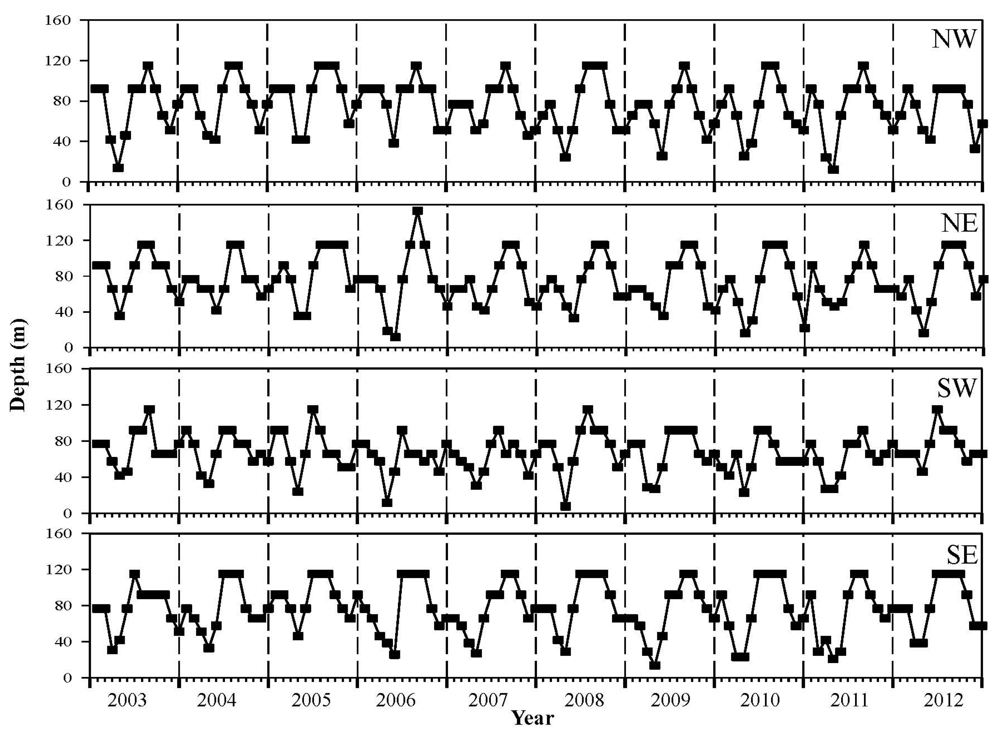
3.1. Temporal Variations of Euphotic Depths

The euphotic depth estimated from the equation referenced in the method section (Zeu = 4.6/Kd(490)) ranged from 7.9 m to 153.3 m for the entire East Sea from 2003 to 2012 (Figure 2). For specific areas, the euphotic depths ranged from 13.5 m to 115.0 m in the SE area and from 7.9 m to 115.0 m in the SW area. Compared with that in the southern East Sea, the range of euphotic depths in the northern East Sea was from 11.5 m to 153.3 m in the NE area and from 12.1 m to 115.0 m in the NW area. In general, the euphotic depth became shallower from January to April, was deepest in August, and then shoaled in November. For the entire East Sea (averaged from the four sub-research areas), the shallowest euphotic depth was found in April with a mean value of 33.9 m (±5.77 m), and the deepest euphotic depth occurred in August with a mean value of 106.9 m (±15.96 m). The second shallowest euphotic depth was observed in November with a mean value of 57.7 m (±5.70 m). There was no specific trend found during the years for the East Sea as a whole.
Figure 2. Monthly variability of euphotic depths for the four sub-research areas in the East Sea from January 2003 to December 2012.
Remotesensing 08 00025 g002

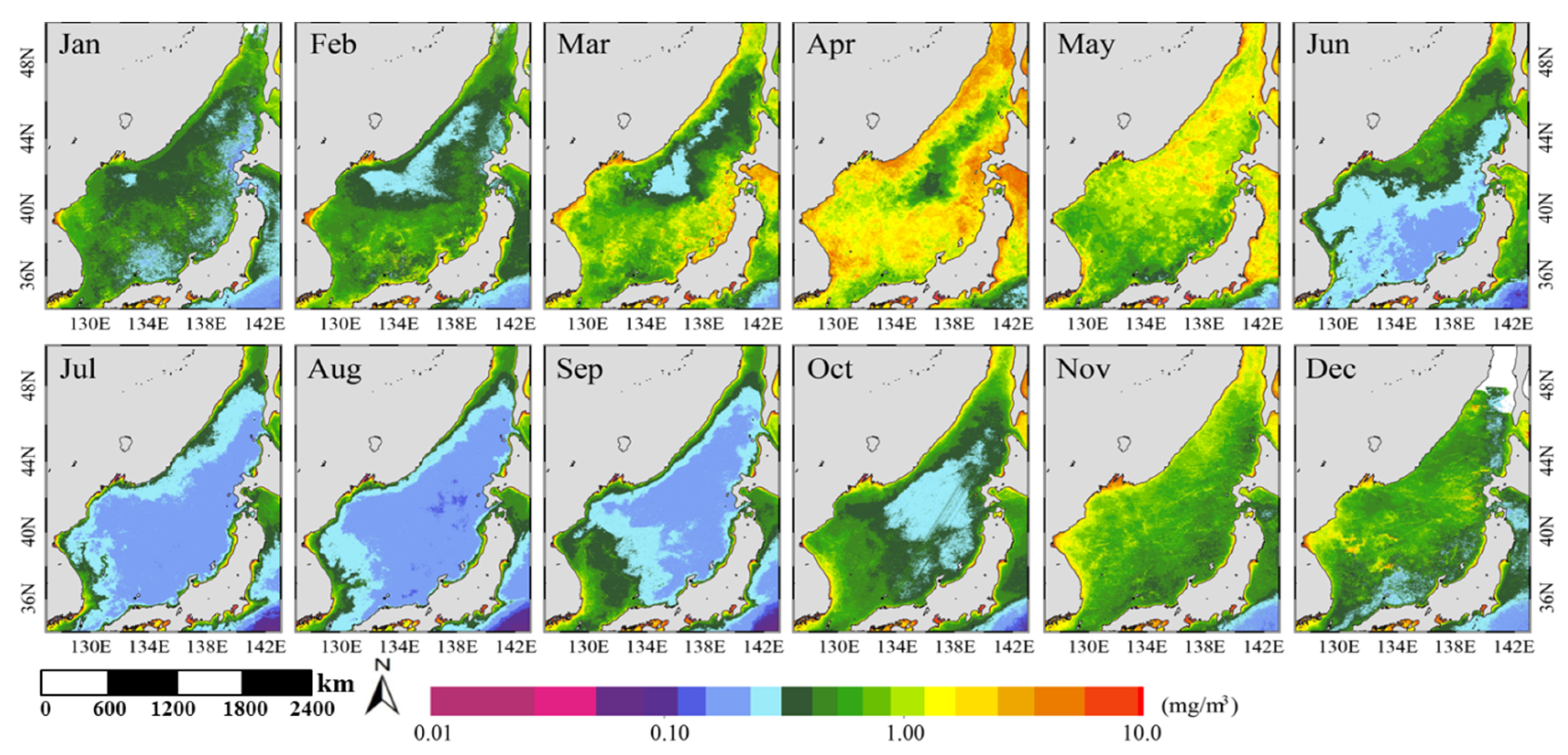
3.2. Spatial and Temporal Variation of MODIS-Derived Chl-a

MODIS-derived climatological monthly (from January 2003 to December 2012) Chl-a maps in the East Sea are shown in Figure 3. The MODIS Chl-a images provided the typical seasonal pattern of phytoplankton biomass in the mid-latitude oceans with the bimodal peaks suggested by Cushing [29] in the East Sea. Spring phytoplankton blooms appeared from March to May, and relatively small fall blooms occurred from October to December, depending on the area. The spring bloom started in the southern area of the East Sea (south of the sub-polar front) and along the coasts in March. The spring bloom peak appeared in April over most of the East Sea, except for the northeastern East Sea. The spring bloom shifted to the northern area of the East Sea (north of the sub-polar front) in May. The lowest Chl-a concentrations occurred in July and August due to strong stratification in the surface water. The fall bloom started in the southwestern East Sea in October and occurred throughout most of the East Sea in November. The Chl-a concentration in the whole region of the East Sea ranged from 0.12 µg·L−1 to 5.09 µg·L−1 from 2003 to 2012 (Figure 3). More specifically, the Chl-a concentration ranged from 0.13 µg·L−1 to 2.51 µg·L−1 in the SE area and from 0.12 µg·L−1 to 5.09 µg·L−1 in the SW area. In comparison, the Chl-a concentration range was from 0.12 µg·L−1 to 4.66 µg·L−1 in the NE area and from 0.15 µg·L−1 to 3.68 µg·L−1 in the NW area. For the entire East Sea (averaged from the four sub-research areas), the spring maximum Chl-a concentration occurred in April, with a median value of 1.59 µg·L−1 (range: 1.15–2.41 µg·L−1), and the summer minimum occurred in August, with a median value of 0.20 µg·L−1 (range: 0.16–0.25 µg·L−1). The fall maximum Chl-a was observed in November, with a median value of 0.59 µg·L−1 (range: 0.39–0.68 µg·L−1), and the winter minimum was observed in January, with a median value of 0.38 µg·L−1 (range: 0.23–0.48 µg·L−1).
Figure 3. Climatological monthly Chl-a maps in the East Sea.
Remotesensing 08 00025 g003

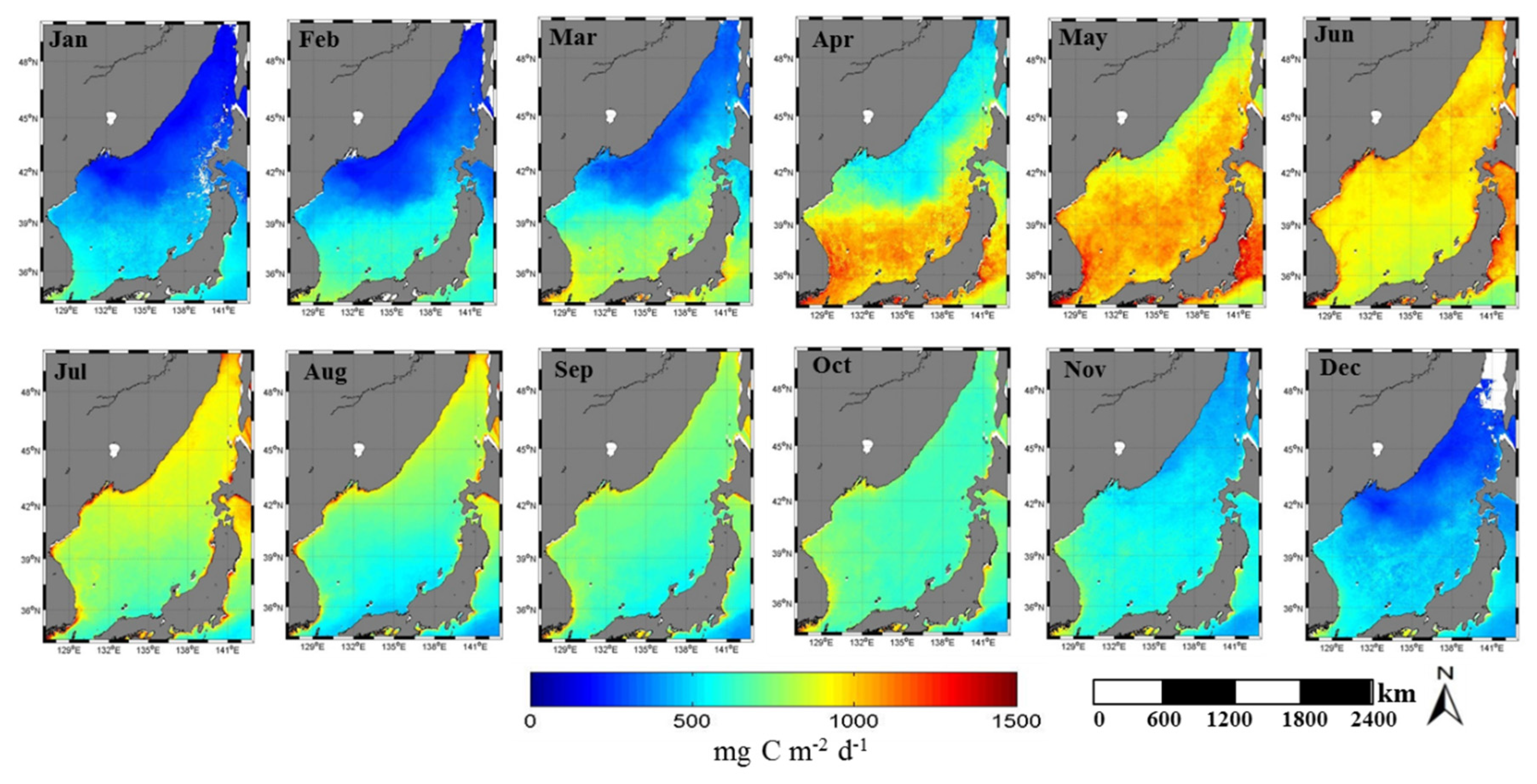
3.3. Spatial and Temporal Variation of MODIS-Derived Primary Productivity

Climatological (January 2003–December 2012) primary productivity data from MODIS for the East Sea were derived using the regional primary productivity model for the East Sea [19]. Figure 4 provides the monthly climatology images from the MODIS-derived primary productivity data in the East Sea. In general, the seasonal pattern of the MODIS primary productivity was somewhat different from that of the MODIS Chl-a, revealing that the primary productivity was higher in spring to early summer (April to June) and lower in winter (December to February). Unlike Chl-a, there was no bimodal peak in the seasonal distribution of the primary productivity (only in the northern areas; however, there was a slight peak in fall in the southern area). The lowest primary productivity occurring in winter was mainly due to the limited light incident for the entire East Sea. More light was available to phytoplankton in spring; therefore, primary productivity increased over the entire East Sea. This increase was especially prominent in the southern area of the sub-polar fronts, which was likely due to the intense stratification. The highest primary productivity appeared in April and May in the southern East Sea (south of the sub-polar front) and in May and June in the northern East Sea. The primary productivity during the summer period (July to August) decreased, but it was not as low as that observed during the winter period. Primary productivity slightly increased in September and October compared with summer and decreased again in November. However, primary productivity in the northern East Sea (north of the sub-polar front) from November to February was generally lower than that in the southern East Sea, which may be related to the deeper mixed layer in the colder water masses and the lower light intensity in the northern latitudes.
Figure 4. Spatial distribution of climatological monthly primary productivity in the East Sea.
Remotesensing 08 00025 g004
Time series of the monthly averages of MODIS-derived primary productivity were generated from January 2003 to December 2012 for the four sub-research areas (NW, NE, SW, and SE) in the East Sea (Figure 5). There was strong seasonal variability in the primary productivity over all of the areas similar to that generated from the climatology monthly primary productivity (Figure 4). No significant inter-annual variability of the primary productivity appeared during the last decade. However, higher primary productivity values were observed in the NW in May 2009 (1181 mg·C·m−2·d−1) and in the SE in May 2006 (1246 mg·C·m−2·d−1). Relatively lower winter primary productivity values were observed in November 2011 (195 mg·C·m−2·d−1) in the NW and in December 2012 (193 mg·C·m−2·d−1) in the NE. Although the primary productivity was highest in April in the southern East Sea (Figure 4), the highest peaks clearly appeared in May 2006 and 2011 in the SE.
Figure 5. Time series of monthly variability in primary productivity for the four sub-research areas in the East Sea from January 2003 to December 2012.
Remotesensing 08 00025 g005
The monthly contributions of primary productivity to the annual production averaged from 2003 and 2012 for the four sub-research areas and the entire East Sea are shown in Table 1. The monthly contributions ranged from 3.8% to 13.2% in the NW and from 3.9% to 13.5% in the NE. In comparison, the monthly contributions ranged from 5.9% to 12.2% in the SW and from 5.6% to 12.5% in the SE. The highest primary productivity level appeared one month later in the northern area than it appeared in the southern area. The contributions during the spring bloom from March to May were 28.4% and 29.5% in the NW and NE, respectively, whereas the contributions were 33.0% and 34.0% in the SW and SE, respectively. The contributions during the summer from June to August were 32.5% and 32.8% in the NW and NE, respectively, whereas the contributions were 25.5% and 25.9% in the SW and SE, respectively. During the fall (from September to November), the contributions were 26.3% and 24.2% in the NW and NE, respectively, whereas the contributions were 22.5% and 21.7% in the SW and SE, respectively. For the winter period (from December to February), the contributions were 12.9% and 13.5% in the NW and NE, respectively, whereas the contributions were 18.8% and 18.1% in the SW and SE, respectively.
Because there was no significant difference in the seasonal primary productivity between the NW and NE in the northern area and the SW and SE in the southern area (Figure 5), we combined the primary productivity values in the NW and NE to form the northern area and the SW and SE to form the southern area (Figure 6). The seasonal pattern of primary productivity averaged over 10 years from 2003 to 2012 in the southern area was somewhat different from that of the northern area. The highest primary productivity was observed in spring followed by summer in the southern area, whereas the highest productivity was observed in summer in the northern area (Figure 6). In general, the primary productivity in the winter and spring seasons was relatively higher in the southern area than in the northern area. The daily primary productivity averaged from the monthly-estimated values in the southern area was 719.7 mg·C·m−2·d−1 (S.D. ± 197.5 mg·C·m−2·d−1, n = 120), which was significantly (paired t-test, p < 0.001) higher than the daily primary productivity in the northern area (632.3 ± 235.1 mg·C·m−2·d−1, n = 120).
Figure 6. Climatological seasonal patterns of primary productivity for the southern and northern areas in the East Sea. Dashed and solid boxes represent annual averaged primary productivity values in the southern and northern areas, respectively. The error bars stand for standard deviation.
Remotesensing 08 00025 g006

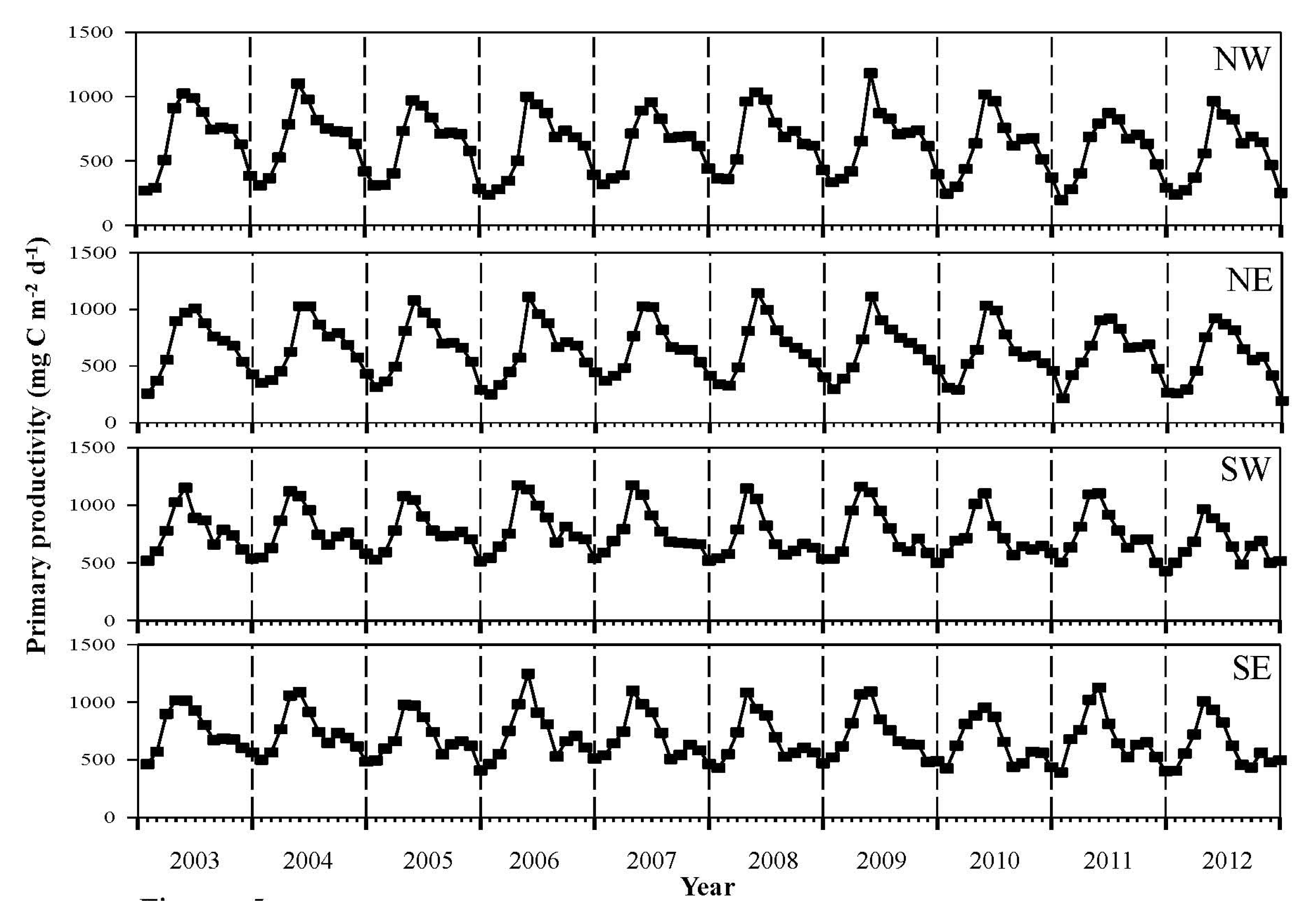
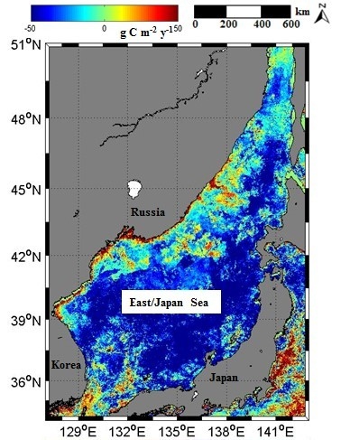
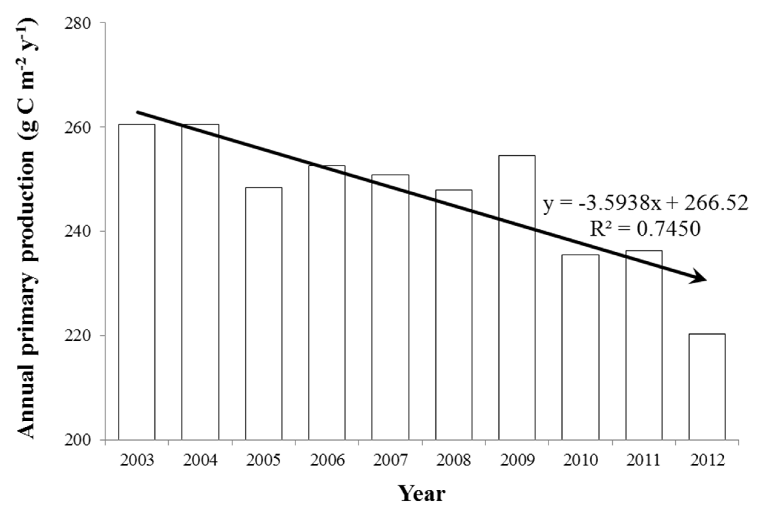
3.4. Long-Term Variation of the Annual Primary Production in the East Sea

To determine the long-term pattern of the primary productivity in the East Sea, the annual primary production values estimated from our daily productivities were plotted for our observation period from 2003 to 2012 (Figure 7). Although there were some oscillations in the annual productivities during the observation years, general decreasing trends were distinct in the northern and southern areas. The decreasing trends were rather similar between the southern and northern areas, although the patterns of productivity were different (Figure 7). For the entire East Sea, the annual primary production also declined during the study period (Figure 8; y = −3.5938x + 266.5, R2 = 0.7450). Primary productivity in the East Sea from 2003 to 2012 decreased a total of 40 g·C·m−2·y−1. The spatial distribution of differences in the annual primary production in the East Sea between 2003 and 2012 is shown in Figure 9. The areas with decreased annual primary production accounted for approximately 79.1% of the total area (mean decreased annual production = 39.3 g·C·m−2·y−1). In comparison, the areas with increased annual primary production contributed 20.9% of the total (mean increased annual production = 25.2 g·C·m−2·y−1). The regions with increased annual production were near the Russian coastal regions in the northwestern coastal area around Russia and the Korea Strait in the southwestern East Sea (Figure 9). However, most of the open ocean areas in the East Sea displayed a decreasing trend in annual primary production.
Figure 7. Long-term patterns of annual primary productions for the southern and northern areas in the East Sea from 2003 to 2012. Dashed and solid lines represent decadal trends in annual primary productions in the southern and northern areas, respectively.
Remotesensing 08 00025 g007
Figure 8. Long-term pattern of annual primary production in the East Sea from 2003 to 2012.
Remotesensing 08 00025 g008
Figure 9. Spatial distribution of annual production difference between 2003 and 2012 in the East Sea.
Remotesensing 08 00025 g009

4. Discussion

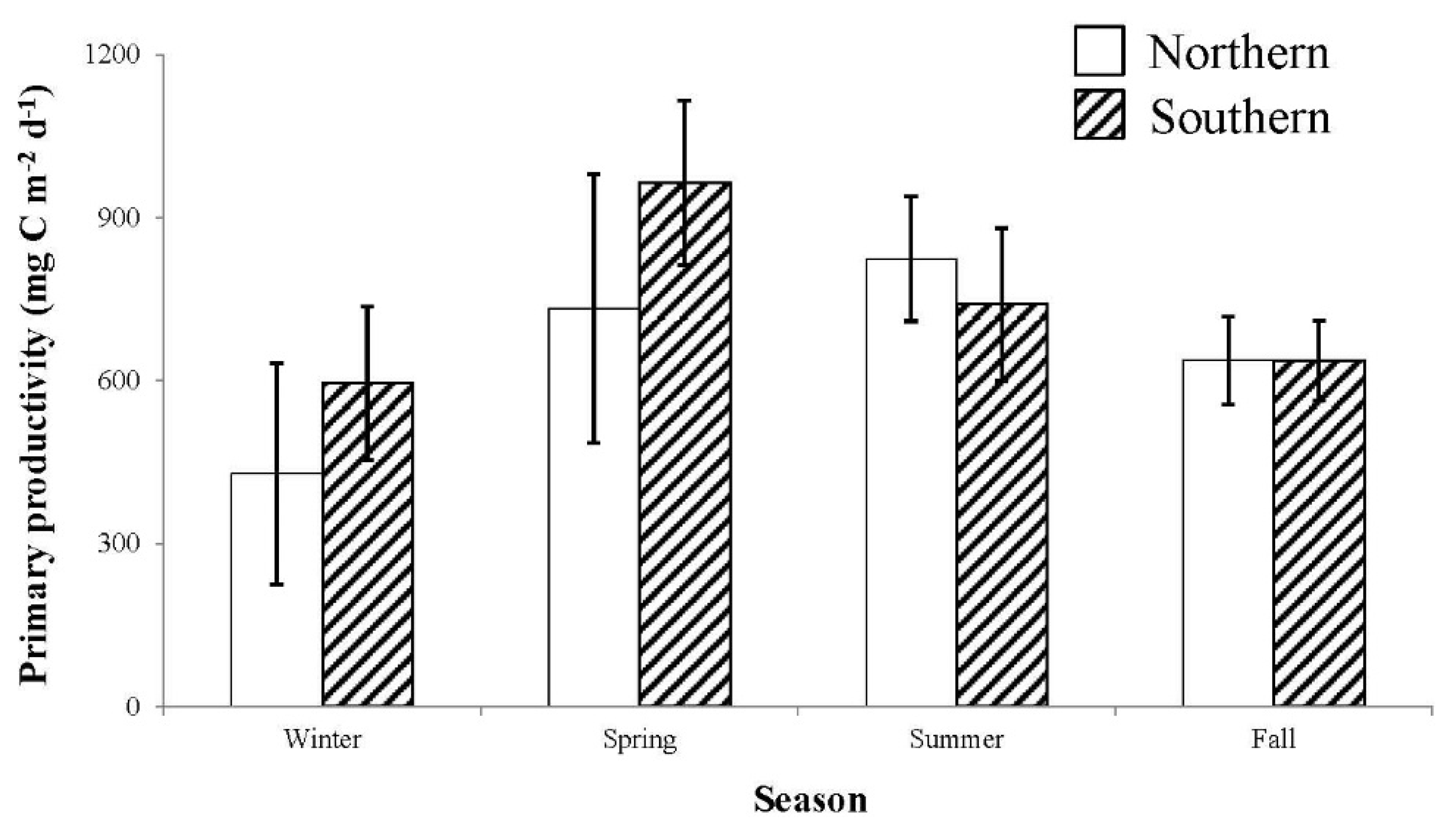
4.1. The Spatial and Seasonal Variations in Chl-a Concentrations in the East Sea

Generally, the seasonal distribution of the MODIS-derived Chl-a concentrations was similar to those presented in previous studies conducted in the East Sea using other ocean color satellite data, such as the Coastal Zone Color Scanner (CZCS) [30] and the SeaWiFS [31]. A distinct seasonal cycle of Chl-a concentrations, especially one showing seasonal patterns of spring and fall booms [20,31], was observed in the East Sea from the time-series ocean color data from 2003 to 2012. However, there were some differences in peak times and magnitudes of Chl-a concentration among the four sub-research areas (Figure 2). High concentrations of Chl-a were observed in spring and fall, and relatively lower Chl-a concentrations were observed in summer and winter, although the patterns of Chl-a concentration were somewhat different among the various regions (Figure 2). In general, spring blooms of phytoplankton started relatively earlier in the southern area than in the northern area in the East Sea.

4.2. Primary Productivity in the East Sea

The monthly contributions to the annual production were not largely variable among the different months in the East Sea, although the contributions of primary productivity in the winter season (from December to February) were relatively lower than those in the other seasons (Table 1). The contribution to the annual primary production in the entire East Sea during the spring bloom (from March to May) was 31.5% and the contribution during the fall bloom (from September to November) was 23.6% (Table 1). Yamada, et al. [19] reported that the contribution of spring and fall blooms was more than 70% of the annual primary production and that the spring and fall blooms had a large effect on the annual primary production in the East Sea. However, the contribution of the spring and fall blooms in this study was 55.1%, which was lower than the value (>70%) found by Yamada et al. [19].
Table 1. The contribution of monthly primary productivity to the annual production for the four sub-research areas (NW, NE, SW, and SE) and the entire East Sea.
MonthNW (%)NE (%)SW (%)SE (%)East Sea (%)
13.83.96.05.64.9
24.24.77.07.25.8
35.76.48.89.27.7
49.59.612.212.311.0
513.213.512.012.512.8
612.412.710.010.611.3
711.011.08.58.79.7
89.19.17.06.67.9
99.58.87.77.28.3
109.18.57.97.78.3
117.66.86.96.87.0
124.95.05.95.75.4
Based on the daily primary productivity estimated using the regional primary productivity algorithm developed by [19], the average annual primary production in the southern area was 262.7 g·C·m−2·y−1 (S.D ± 17.6 g·C·m−2·y−1, n = 10) which is significantly (paired t-test, p < 0.001) higher than the value (230.8 ± 13.5 g·C·m−2·y−1, n = 10) in the northern area of the East Sea. The East Sea can be divided into southern and northern regions based on the sub-polar front (Figure 1; [32]). The southern and northern regions in the East Sea are hydrographically and biologically very distinct; the southern region has more tropical biological characteristics and species [33]. The higher annual primary production in the southern area compared to the northern area in this study was consistent with results from previous studies in the East Sea [18,31], although Nishimura [34] and Nagata [35] reported that the primary productivity was higher in the northern area than in the southern area.
In this study, the average annual primary production in the entire East Sea was 246.8 g·C·m−2·y−1, which was relatively higher than the previously reported values [18,34,36]. Nishimura [34] reported that the range of annual primary production was 75–200 g·C·m−2·y−1 based on several measurements and estimates around Japan. Based on SeaWiFS data, Yamada et al. [19] reported a range of 161–222 g·C·m−2·y−1, depending on the different areas in the East Sea. Further, Yoo and Kim [36] reported a similar annual primary production of 240 g·C·m−2·y−1 in the East Sea based on the CZCS data from 1978 to 1986. However, Yoo and Kim [36] estimated annual primary production based on the VGPM developed by Behrenfeld and Falkowski [17]. The depth integrated primary productivity estimated by the VGPM tends to be inflated by the overestimation of high Chl-a concentrations [27]; therefore, the annual primary production reported by Yoo and Kim [36] of 240 g·C·m−2·y−1, which might be an overestimation, was lower than the average annual primary production in this study (246.8 g·C·m−2·y−1). Our estimated annual primary production (246.8 g·C·m−2·y−1) in the East Sea was considerably higher than the Mediterranean Sea values, which were based on the CZCS data (range: 109–158 g·C·m−2·y−1) [37], though the Mediterranean has similar environmental conditions as the East Sea.

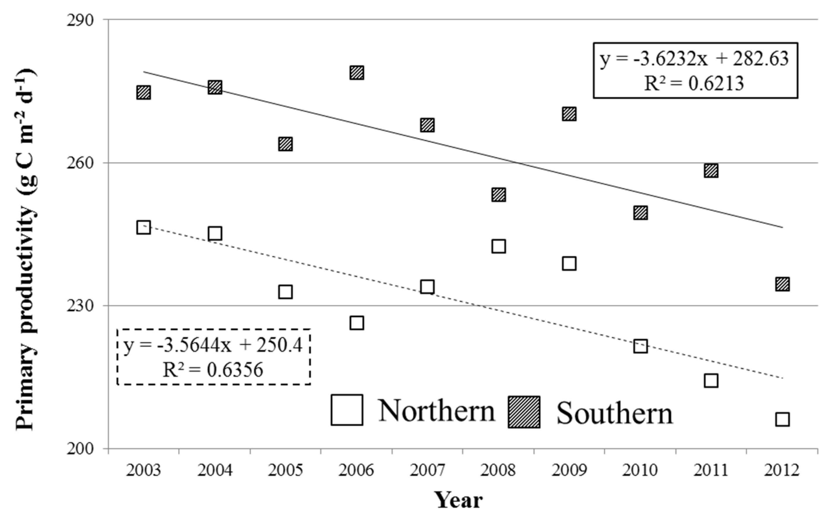
4.3. Long-Term Pattern of the Annual Primary Production in the East Sea

The annual primary production in the entire East Sea declined during the study period starting in 2003 (Figure 8). The Pearson correlation coefficient with time is significant at p = 0.01 from 2003 to 2012. However, the spatial patterns of the decadal trend in the annual primary production differed among regions (Figure 9). The annual primary production decreased in wider areas of the East Sea, which was mostly the open ocean. In contrast, the annual primary production increased near the Russian coastal regions in the northwestern coastal area around Russia and the southern coastal area in the East Sea. Although PAR and euphotic depth are also important components for controlling the primary production in our productivity algorithm, we did not find any strong relationship between the declined annual primary production and PAR and euphotic depth in this study. An increased SST may have caused the increased stratification of the surface mixed layer and, consequently, reduced the entrainment of major nutrients into the upper euphotic layer [38,39]. In fact, the SST in the East Sea rapidly increased over several decades [7,8,40]. Recently, Jo et al. [40] reported that the rate of the SST increase was 0.041 °C·y−1 in the east coast of Korea, which was much faster than the global average (0.005 °C·y−1). However, no substantial increased SST was observed in this study during our investigation period (2003–2012), most likely because the observation period was not long enough to detect any small changes in the SST [13]. Gregg et al. [39] argued that increased temperature and shallower mixed layers via surface stratification could result in increased Chl-a concentrations in early spring and that more severe nutrient exhaustion in late spring and summer could reduce the Chl-a concentrations and, consequently, annual primary production [41]. In fact, the concentrations of major inorganic nutrients decreased in euphotic water layers (0–50 m water depth) in the Ulleung Basin (located in the middle of the East Sea) during our observation period [13]. The decrease in nitrate concentrations was also distinct during both the summer time and the winter season in the study region from 2003 to 2012 [13].
Various authors found a strong correlation between the annual primary production in the East Sea and the PDO [5,13,42]. Chiba et al. [5] suggested that the reduced warm Tsushima surface current and shoaling cold subsurface water during the negative phase of PDO caused a reduction in lower-trophic level productivity due to the nutrient depletion triggered by strong stratification in the East Sea. Joo et al. [13] found a strong correlation between PDO and nutrient concentration integrated from the surface to a water depth of 50 m in the Ulleung Basin. Therefore, the recent declining trend of annual primary production from 2003 to 2012 in this study could be part of an oscillation pattern of annual primary production in the East Sea governed by PDO, not solely a decreasing trend.

5. Conclusions

The East Sea has very dynamic environmental conditions caused by many physical properties such as a warm–cold strong fronts, many eddies, and frequent coastal upwellings. Over recent decades, few reports have been made of the biological change in the East Sea, although substantial marine environmental changes have been observed. In this study, we found that the annual primary production of phytoplankton had been noticeably decreasing over the recent decade, based on the recent decadal primary productivity derived by Moderate-Resolution Imaging Spectroradiometer (MODIS) algorithm. Increasing temperature and subsequent shallower mixed layers and an oscillation pattern strongly governed by the Pacific Decadal Oscillation (PDO) could be potential causes for the decline in the annual production of the East Sea. During the recent decade from 2003 to 2012 in this study, the annual primary production decreased approximately 40 g·C·m−2·y−1 in the East Sea. This decrease in annual primary production would lead to a decrease in fishery landings (approximately 9.5 kg·ha−1·y−1) in the East Sea based on Nixon and Thomas [43]. Our observation holds an important implication for future fishery management in the East Sea. This aspect warrants further intensive interdisciplinary field studies to better understand the declining trend of annual primary production and the subsequent effects on the marine ecosystem in the East Sea.

Acknowledgments

We especially thank the anonymous reviewers who greatly improved an earlier version of the manuscript. This research was a part of the project entitled “Long-term change of structure and function in marine ecosystems of Korea” and “Development of Korea Operational Oceanographic System (KOOS)” funded by the Ministry of Oceans and Fisheries, Korea.

Author Contributions

HuiTae Joo and Sang Heon Lee are responsible for the overall paper while all other authors contributed equally to the work. HuiTae Joo, SeungHyun Son, Sang Heon Lee, and Chang-Keun Kang designed the overall study and prepared this paper. HuiTae Joo, Jung-Woo Park and SeungHyun Son processed the major satellite data sources. Jae Jung Kang, Jin-Yong Jeong, and Chung Il Lee helped with data analysis and manuscript preparation.

Conflicts of Interest

The authors declare no conflict of interest.

References

  1. Onitsuka, G.; Yanagi, T.; Yoon, J.H. A numerical study on nutrient sources in the surface layer of the Japans Sea using a coupled physical-ecosystem model. J. Geophys. Res. 2007, 112, C05042. [Google Scholar] [CrossRef]
  2. Kang, Y.S.; Kim, J.Y.; Kim, H.G.; Park, J.H. Long_term changes in zooplankton and its relation_ship with squid, Todarodes pacificus, catch in Japan/East Sea. Fish. Oceanogr. 2002, 11, 337–346. [Google Scholar] [CrossRef]
  3. Kim, D.; Yang, E.J.; Kim, K.H.; Shin, C.-W.; Park, J.; Yoo, S.; Hyun, J.-H. Impact of an anticyclonic eddy on the summer nutrient and Chl-a a distributions in the Ulleung Basin, East Sea (Japan Sea). ICES J. Mar. Sci. 2012, 69, 23–29. [Google Scholar] [CrossRef]
  4. Lim, J.-H.; Son, S.; Park, J.-W.; Kwak, J.H.; Kang, C.-K.; Son, Y.B.; Kwon, J.-N.; Lee, S.H. Enhanced biological activity by an anticyclonic warm eddy during early spring in the East Sea (Japan Sea) detected by the geostationary ocean color satellite. Ocean Sci. J. 2012, 47, 377–385. [Google Scholar] [CrossRef]
  5. Chiba, S.; Aita, M.N.; Tadokoro, K.; Saino, T.; Sugisaki, H.; Nakata, K. From climate regime shifts to lower-trophic level phenology: Synthesis of recent progress in retrospective studies of the western North Pacific. Prog. Oceanogr. 2008, 77, 112–126. [Google Scholar] [CrossRef]
  6. Kim, K.-R.; Kim, K.; Kang, D.-J.; Park, S.Y.; Park, M.-K.; Kim, Y.-G.; Min, H.S.; Min, D. The East Sea (Japan Sea) in change: A story of dissolved oxygen. Mar. Technol. Soc. J. 1999, 33, 15–22. [Google Scholar] [CrossRef]
  7. Kim, K.; Kim, K.-R.; Min, D.-H.; Volkov, Y.; Yoon, J.-H.; Takematsu, M. Warming and structural changes in the East (Japan) Sea: A clue to future changes in global oceans? Geophys. Res. Lett. 2001, 28, 3293–3296. [Google Scholar] [CrossRef]
  8. Kang, D.J.; Park, S.; Kim, Y.G.; Kim, K.; Kim, K.-R. A moving-boundary box model (MBBM) for oceans in change: An application to the East/Japan Sea. Geophys. Res. Lett. 2003, 30, 1299. [Google Scholar] [CrossRef]
  9. Sasaoka, K.; Chiba, S.; Saino, T. Climatic forcing and phytoplankton phenology over the subarctic North Pacific from 1998 to 2006, as observed from ocean color data. J. Geophys. Lett. 2011, 38, L15609. [Google Scholar] [CrossRef]
  10. Chiba, S.; Batten, S.; Sasaoka, K.; Sasai, Y.; Sugisaki, H. Influence of the Pacific Decadal Oscillation on phytoplankton phenology and community structure in the western North Pacific. Geophys. Res. Lett. 2012, 39, L15603. [Google Scholar] [CrossRef]
  11. Chiba, S.; Saino, T. Variation in mesozooplankton community structure in the Japan/East Sea (1991–1999) with possible influence of the ENSO scale climatic variability. Prog. Oceanogr. 2002, 213, 23–25. [Google Scholar] [CrossRef]
  12. Zhang, C.I.; Lee, J.B.; Young, I.S.; Yoon, S.C.; Kim, S. Variations in the abundance of fisheries resources and ecosystem structure in the Japan/East Sea. Prog. Oceanogr. 2004, 61, 245–265. [Google Scholar] [CrossRef]
  13. Joo, H.; Park, J.W.; Son, S.; Noh, J.-H.; Jeong, J.-Y.; Kwak, J.H.; Saux-Picart, S.; Choi, J.H.; Kang, C.-K.; Lee, S.H. Long-term annual primary production in the Ulleung Basin as a biological hot spot in the East/Japan Sea. J. Geophys. Res. Oceans 2014, 119, 3002–3011. [Google Scholar] [CrossRef]
  14. Grebmeier, J.M.; Bluhm, B.A.; Cooper, L.W.; Danielson, S.L.; Arrigo, K.R.; Blanchard, A.I.; Clarke, J.T.; Day, R.H.; Frey, K.E.; Gradinger, R.R.; et al. Ecosystem characteristics and processes facilitating persistent macrobenthic biomass hotspots and associated benthivory in the Pacific Arctic. Prog. Oceanogr. 2015, 136, 92–114. [Google Scholar] [CrossRef]
  15. Lee, S.H.; Joo, H.T.; Lee, J.H.; Kang, J.J.; Lim, J.-H.; Yun, M.S.; Lee, J.H.; Kang, C.-K. Potential overestimation in primary and new productivitys of phytoplankton from a short time incubation method. Ocean Sci. J. 2015, 50, 509–517. [Google Scholar] [CrossRef]
  16. Platt, T.; Sathyendranath, S. Oceanic primary productivity: Estimation by remote sensing at local and regional scales. Science 1988, 241, 1613–1620. [Google Scholar] [CrossRef] [PubMed]
  17. Behrenfeld, M.J.; Falkowski, P.G. Photosynthetic rates derived from satellite-based Chl-a concentration. Limnol. Oceanogr. 1997, 42, 1–20. [Google Scholar] [CrossRef]
  18. Son, S.; Campbell, J.; Dowell, M.; Yoo, S.; Noh, J. Primary productivity in the Yellow Sea determined by ocean color remote sensing. Mar. Ecol. Prog. Ser. 2005, 303, 91–103. [Google Scholar] [CrossRef]
  19. Yamada, K.; Ishizaka, J.; Nagata, H. Spatial and temporal variability of satellite primary productivity in the Japan Sea from 1998 to 2002. J. Oceanogr. 2005, 61, 857–869. [Google Scholar] [CrossRef]
  20. Lee, S.H.; Son, S.; Dahms, H.-U.; Park, J.W.; Lim, J.-H.; Noh, J.-H.; Kwon, J.-I.; Joo, H.T.; Jeong, J.Y.; Kang, C.-K. Decadal changes of phytoplankton Chl-a-a in the East Sea/Sea of Japan. Oceanology 2014, 6, 771–779. [Google Scholar] [CrossRef]
  21. Helbling, E.W.; Villafañe, V.E. Phytoplankton and primary productivity. In Fisheries and Aquaculture; Safran, P., Ed.; Eolss Publishers: Paris, France, 2009; Volume 5. [Google Scholar]
  22. Wassmann, P.; Duarte, C.M.; Agusti, S.; Sejr, M.K. Footprints of climate change in the Arctic marine ecosystem. Glob. Chang. Biol. 2011, 17, 1235–1249. [Google Scholar] [CrossRef]
  23. Arrigo, K.R.; Dijken, G.L.V. Continued increases in Arctic Ocean primary productivity. Prog. Ocenogr. 2015, 136, 60–70. [Google Scholar] [CrossRef]
  24. Falkowski, P.G.; Rave, J.A. Aquatic Photosynthesis, 2nd ed.; Blackwell: Oxford, UK, 1997. [Google Scholar]
  25. Yoder, J.A.; Kennelly, M.A. Seasonal and ENSO variability in global ocean phytoplankton Chl-a derived from 4 years of Sea WiFS measurements. Glob. Biogeochem. Cycles 2003, 17, 1112. [Google Scholar] [CrossRef]
  26. Kameda, T. Studies on oceanic primary productivity using ocean color remote sensing data. Bull. Fish. Res. Agency 2003, 9, 118–148. [Google Scholar]
  27. Kameda, T.; Ishizaka, J. Size-fractionated primary productivity estimated by a two-phytoplankton community model applicable to ocean color remote sensing. J. Oceanogr. 2005, 61, 663–672. [Google Scholar] [CrossRef]
  28. Kirt, J.T.O. Light and Photosynthesis in Aquatic Ecosystems, 2nd ed.; Cambridge University Press: Cambridge, UK, 1994. [Google Scholar]
  29. Cushing, D.H. The seasonal variation in oceanic productivity as a problem in population dynamics. J. Cons. Int. Explor. Mer. 1959, 24, 455–464. [Google Scholar] [CrossRef]
  30. Son, S. The Chl-a Pigment Distribution in the East/Japan Sea Observed by Coastal Zone Color Scanner (CZCS). Master’s Thesis, Pusan National University, Busan, Korea, 1998. [Google Scholar]
  31. Yamada, K.; Ishizaka, J.; Yoo, S.; Kim, H.-C.; Chiba, S. Seasonal and interannual variability of sea surface Chl-a a concentration in the Japan/East Sea (JES). Prog. Oceanogr. 2004, 61, 193–211. [Google Scholar] [CrossRef]
  32. Senjyu, T. The Japan Sea intermediate water; characteristics and circulation. J. Oceanogr. 1999, 55, 111–122. [Google Scholar] [CrossRef]
  33. Ashjian, C.J.; Davis, C.S.; Gallager, S.M.; Alatalo, P. Characterization of the zooplankton community, size composition, and distribution in relation to hydrography in the Japan/East Sea. Deep Sea Res. II 2005, 52, 1363–1392. [Google Scholar] [CrossRef]
  34. Nishimura, S. Okhotsk Sea, Japan Sea, East China Sea. In Estuaries and Enclosed Seas; Ketchum, B.H., Ed.; Elsevier Scientific Publishing Company: Amsterdam, The Netherlands, 1983; pp. 375–401. [Google Scholar]
  35. Nagata, H. The relationship between Chl-a a and transparency in the southern Japan Sea. Proc. Jpn. Sci. Coun. Fish. Resour. 1992, 28, 29–44. [Google Scholar]
  36. Yoo, S.; Kim, H.C. Primary productivity in the East Sea. In The Plankton Ecology of Korean Coastal Waters; Choi, J.K., Ed.; Dongwha Press: Seoul, Korea, 2003; pp. 96–111. [Google Scholar]
  37. Estrada, M. Primary productivity in the northwestern Mediterranean. Sci. Mar. 1996, 60, 55–64. [Google Scholar]
  38. Sarmiento, J.L.; Hughes, T.M.C.; Stouffer, R.J.; Manabe, S. Simulated response of the ocean carbon cycle to anthropogenic climate warming. Nature 1998, 393, 245–249. [Google Scholar] [CrossRef]
  39. Gregg, W.W.; Conkright, M.E.; Ginoux, P.; O’Reilly, J.E.; Casey, N.W. Ocean Primary productivity and climate: Global decadal changes. Geophys. Res. Lett. 2003, 15, 1809. [Google Scholar] [CrossRef]
  40. Jo, Y.H.; Breaker, L.C.; Tseng, Y.-H.; Yeh, S.-W. A temporal multiscale analysis of the waters off the east coast of south Korea over the past four decades. Terr. Atoms. Ocean. Sci. 2014, 3, 415–434. [Google Scholar] [CrossRef]
  41. Gregg, W.W.; Conkright, M.E. Decadal changes in global ocean Chl-a. Geophys. Res. Lett. 2002, 29, 130. [Google Scholar] [CrossRef]
  42. Yatsu, A.; Chiba, S.; Yamanaka, Y.; Ito, S.I.; Shimize, Y.; Kaeriyama, M.; Watanabe, Y. Climate forcing and the Kuroshio/Oyashio ecosystem. ICES J. Mar. Sci. 2013, 70, 922–933. [Google Scholar] [CrossRef]
  43. Nixon, S.; Thomas, A. On the size of the Peru upwelling ecosystem. Deep Sea Res. I 2001, 48, 2521–2528. [Google Scholar] [CrossRef]

