Article

Mapping Rice Cropping Systems in Vietnam Using an NDVI-Based Time-Series Similarity Measurement Based on DTW Distance

1
State Key Laboratory of Resources and Environmental Information System, Institute of Geographic Sciences and Natural Resources Research, Chinese Academy of Sciences, Beijing 100101, China
2
College of Resources and Environment, University of Chinese Academy of Sciences, Beijing 100049, China
3
Key Laboratory of Ecosystem Network Observation and Modeling, Institute of Geographic Sciences and Natural Resources Research, Chinese Academy of Sciences, Beijing 100101, China
4
Department of Geography and Anthropology, Louisiana State University, Baton Rouge, LA 70803, USA
5
Jiangsu Center for Collaborative Innovation in Geographic Information Resource Development and Application, Nanjing 210023, China
*
Author to whom correspondence should be addressed.
Remote Sens. 2016, 8(1), 19; https://doi.org/10.3390/rs8010019
Submission received: 22 October 2015 / Revised: 15 December 2015 / Accepted: 21 December 2015 / Published: 8 January 2016

Abstract

:
Normalized Difference Vegetation Index (NDVI) derived from Moderate Resolution Imaging Spectroradiometer (MODIS) time-series data has been widely used in the fields of crop and rice classification. The cloudy and rainy weather characteristics of the monsoon season greatly reduce the likelihood of obtaining high-quality optical remote sensing images. In addition, the diverse crop-planting system in Vietnam also hinders the comparison of NDVI among different crop stages. To address these problems, we apply a Dynamic Time Warping (DTW) distance-based similarity measure approach and use the entire yearly NDVI time series to reduce the inaccuracy of classification using a single image. We first de-noise the NDVI time series using S-G filtering based on the TIMESAT software. Then, a standard NDVI time-series base for rice growth is established based on field survey data and Google Earth sample data. NDVI time-series data for each pixel are constructed and the DTW distance with the standard rice growth NDVI time series is calculated. Then, we apply thresholds to extract rice growth areas. A qualitative assessment using statistical data and a spatial assessment using sampled data from the rice-cropping map reveal a high mapping accuracy at the national scale between the statistical data, with the corresponding R2 being as high as 0.809; however, the mapped rice accuracy decreased at the provincial scale due to the reduced number of rice planting areas per province. An analysis of the results indicates that the 500-m resolution MODIS data are limited in terms of mapping scattered rice parcels. The results demonstrate that the DTW-based similarity measure of the NDVI time series can be effectively used to map large-area rice cropping systems with diverse cultivation processes.

Graphical Abstract

1. Introduction

Rice is the most important crop in Vietnam and accounts for 40% of gross agricultural production in the country [1,2,3]. As a result of its suitable climate, Vietnam has increased its rice production continually since 1995 (FAO, 2012), eventually becoming the second-largest rice exporting country in 2012 [4]. Effective rice monitoring is essential for supporting policy making with accurate information concerning rice-growing areas, estimation of production, and seasonal cropping patterns to achieve increased economic development and food security.
Remote sensing represents a reliable and effective approach to assessing crop growth and production at various scales [5,6,7,8,9,10,11]. To map the distribution of rice fields, moderate-scale analyses often use high to medium spatial resolution (6 to 30 m) optical data acquired from Landsat [12,13], Systeme Probatoire d’Observation de la Terre (SPOT) [14], and Indian Remote Sensing Satellite (IRS) [15]. Regional- and global-scale analyses commonly apply coarser spatial resolution imagery with larger swath widths such as imagery from the Advanced Very High Resolution Radiometer (AVHRR), Moderate Resolution Imaging Spectroradiometer (MODIS), and SPOT VEGETATION (SPOT VGT) [16]. Various classification methods, such as unsupervised classification and supervised classification, have been adopted to map rice systems [17,18]. The phase analysis method using time-series VI indicates the greenness of vegetation growing in different phases. Notably, Xiao et al. [19,20], using LSWI, EVI, and NDVI information derived from MODIS data to map rice systems in China and Southeast Asia based on the fact that the land surface includes a mixture of surface water and green rice plants during the flooding and rice transplanting period, found that crops generally exhibit distinct growth characteristics during different seasons [21]. Gumma et al. [22] used a spectral similarity value to evaluate the similarities between the NDVI time series and rice pixels grouped using the 500-m resolution MODIS data and mapped the Bangladesh rice cultivation distribution. Chen et al. [23] applied a linear mixture model with 250-m resolution MODIS NDVI data to classify the rice-cropping systems in the Mekong Delta of Vietnam. Kontgis et al. [24] recently mapped rice paddy extent and intensification in the Mekong River Delta with dense time stacks of Landsat data (high to medium spatial resolution data); in this project, their methods drew upon other methods developed by Xiao et al. using MODIS time-series data [19,20].
Several factors related to rice cropping and the local environment present challenges for rice mapping using low-temporal-resolution remote sensing data such as TM data and SPOT data. First, the suitable sunlight, heat, and water conditions in Southeast Asia allow for a flexible rice planting schedule. The variation in rice-growing periods produces mixed pixels in remote sensing data. Second, these satellites’ long revisit cycles of 16 days to 26 days impose limitations on obtaining real-time images. Third, the cloudy and rainy weather conditions of Southeast Asia often produce heavy cloud coverage in images and significantly decrease the availability of high-quality images. According to the statistics in this study, within the Vietnamese territory, the probability of obtaining images with less than 20% cloud cover is less than 5% (according to cloud detection applied to TM images in Vietnam in 2010) and during the monsoon season of Vietnam (May to November, namely, days 120 to days 304), the mean cloud coverage was 47% (Figure 1). As a result, remote sensing classification methods based on a single temporal vegetation index are limited. However, crops of the same type have the same phenology and share certain NDVI curve characteristics. Identifying crop cycles from high-temporal-resolution images continues to represent a promising approach [25]. To mine the temporal characteristics of rice growth from high-temporal-resolution data, we applied a Dynamic Time Warping (DTW) similarity measure to time-series NDVI data derived from MODIS imagery to extract rice cultivated areas.
The time-series similarity measure is widely used in many fields primarily to describe the characteristics of data variations over time. Time-series similarity research has become a core component of time-series data mining. Time-series similarity also has numerous prospects in such remote sensing applications as the extraction of vegetation areas, and such data have many applications. For example, Geerken and Zaitchik [25] classified pasture vegetation using time-series similarity based on the Fourier transform method with MODIS NDVI time series. Gumma et al. [22] mapped seasonal rice cropland using 500-m-resolution MODIS data based on a spectral matching technique. DTW (dynamic time warping) is commonly used to compare the similarity of two given time series under certain conditions. The DTW distance, which is the measure of the DTW-based similarity of two time series, was originally applied to the matching of text data in the field of speech processing; visual pattern recognition, curve similarity measurement, and time-series classification and clustering in the field of speech recognition; medical analysis; and moving object identification. Research has shown that this algorithm, which is based on nonlinear bending, can obtain high matching accuracy [26,27]. The DTW distance can also be integrated into many classification techniques such as nearest neighbor classifiers, support vector machines, and neural networks to replace the Euclidean distance and thus improve classification accuracy [28,29,30,31,32,33,34]. Petitjean et al. tested the K-means algorithm with DTW and DTW barycenter averaging (DBA) on satellite image time-series analysis and used a K-means-based algorithm and DTW distance to cluster pixels from a SPOT image time series [35,36]. Izakian et al. evaluated Fuzzy C-means (FCM) clustering and Fuzzy C-medoids (FCMdd) clustering and improved both with a proposed hybrid technique [37]. Jeong et al. proposed a new kernel function based on a weighted DTW distance for support vector machines for classifying non-aligned time-series data [38].
Figure 1. Cloud coverage in images. Among the 46 MODIS images, the cloud coverage of 33 MODIS images exceeds 20%, and that of 16 images exceeds 40%. During the rainy season of Vietnam (May to November, namely, day 120 to day 304), the mean cloud coverage was 47%.
Remotesensing 08 00019 g001
The main objective of this paper is to map rice cropping systems in Vietnam for the year 2010 according to the similarity between the NDVI time series of every pixel and the standard rice growth NDVI time series. We use the DTW distance, which finds the optimal alignment (or coupling) between two sequences of numerical values and captures flexible similarities by aligning the coordinates inside both sequences, to address irregular rice growth NDVI time-series data (caused by the flexible rice planting schedule in Vietnam). We verified the performance of the DTW-distance-based similarity method applied to mapping rice-growing systems in Vietnam, and the results demonstrated that this method can be applied to the determination of rice cropping systems over wide areas in which rice planting schedules are flexible.
The study is structured as follows. Section 2 introduces the study area and utilized dataset and discusses why we chose the MOD09A1 data set and NDVI time series. Section 3 introduces three filtering algorithms in the TIMESAT software and shows how we compare them. Section 4 discusses how we constructed the standard rice growth NDVI time-series and the DTW theory and how we applied the DTW similarity measure to the NDVI time-series data to extract rice cultivation areas. Section 5 presents the results. We map the distribution of single rice cropping, double rice cropping, and triple rice cropping in Vietnam using a threshold in the DTW distance map. Then we use the statistical data combined with the sampled data from field surveys and Google Earth sampling data to analyze the accuracy of the rice distribution map. Section 6 includes some conclusions and discusses future work.

2. Study Area and Materials

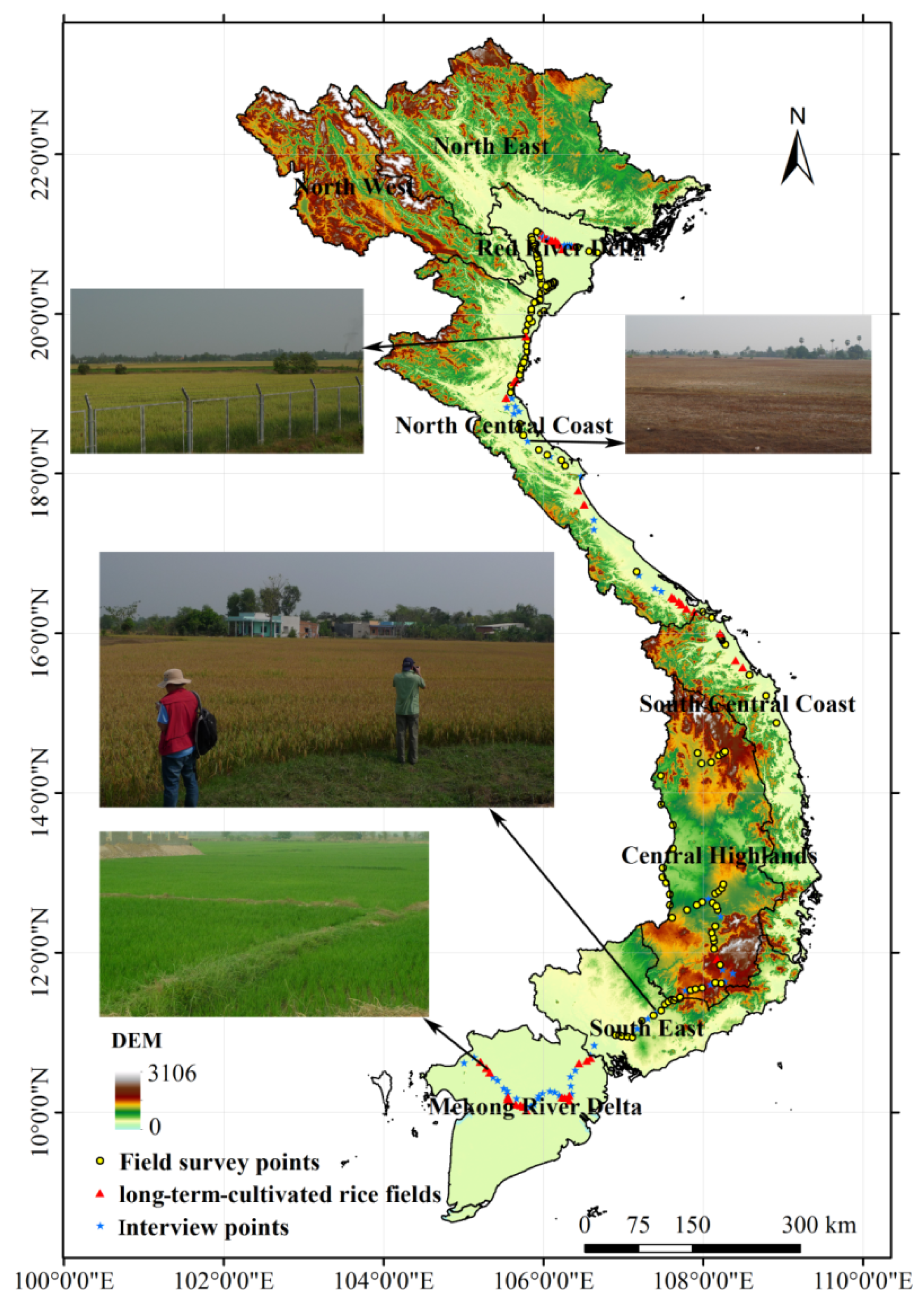
2.1. Brief Introduction to the Study Area

The study area of this research includes the entire country of Vietnam. Vietnam is located in the eastern region of the Indo-China peninsula, extending from 8°10′ to 23°24′N and from 102°09′ to 109°30′E and covering an area of 329,556 km2. Vietnam is long and narrow, with high elevations in the west and low elevations in the east. Vietnam experiences a tropical monsoon climate characterized by high temperatures and rainy seasons. The annual average temperature is approximately 24 °C, and the average annual rainfall ranges from 1500 mm to 2000 mm.
Vietnam is a traditional agricultural country; the agricultural population accounts for approximately 75 percent of the total population. Cultivated land and forest land constitute 60% of the total area. Food crops include rice, corn, potatoes, sweet potatoes, and cassava, and economic crops include coffee, rubber, cashew nuts, peanuts, silk, and tea.
According to the topography, soil, and climate conditions, agricultural activity can be divided into eight agricultural ecological sections: North Central Coast, North East, Mekong River Delta, Red River Delta, South East, South Central Coast, North West, and Central Highlands (Figure 2). In Vietnam, much of the rice cultivation is concentrated in two river deltas: the Mekong (over half of the country’s rice area) and Red deltas. The planted area in 2000 was approximately 7.6 million ha, and the cropping intensity (ratio of sown area to land area for a given crop) is the highest in the world [39]. The high cropping intensity is largely due to the planting of the triple rice crops that are common in much of the Mekong Delta area [40]. According to Son et al. [41], five cropping seasons per year are observed in Vietnam: the rainy season (July–August to December–January), the winter–spring season (November–December to February–March), the spring–summer season (March–April to May–June), the summer–autumn season (April–May to July–August), and the autumn–winter season (July–September to October–December). The rain-fed rice cropping system using long-duration varieties (160–180 days) is invariably applied in areas that are subject to soil and water constraints, whereas irrigated rice cropping systems using short-duration varieties (90–100 days) are applied in areas where irrigation conditions are favorable.
Figure 2. Field survey in Vietnam.
Remotesensing 08 00019 g002

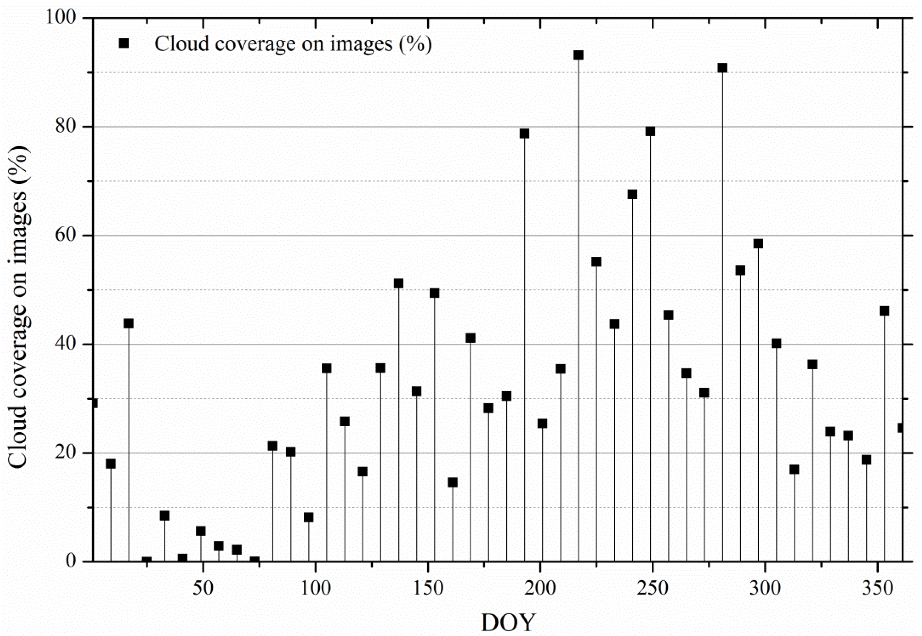
2.2. MODIS NDVI Time-Series Data

MODIS imagery was acquired from NASA’s (National Aeronautics and Space Administration) website [42]; specifically, the surface reflectance MOD09A1 eight-day composite products named “MODIS/Terra surface reflectance 8-day Global 500 m SIN GRID V005” for 2010 were used. We obtained the first two bands of the MOD09A1 data for NDVI calculation as well as the corresponding Quality Assessment (QA) data. Five tiles (i.e., h27v06, h27v07, h28v06, h28v07, and h28v08) covered the entire territory of Vietnam. The MOD09A1 data products were systematically corrected for the effects of gaseous and aerosol scattering. Each pixel contains the optimal quality L2G observation data for eight days with information about the highest observation range and minimum observation angle (without clouds or cloud shadows) [43].
The MOD13 datasets provided the level 2G (gridded) surface reflectance and temporally composited these values to generate the 16-day, 250/500-m, or 1-km VI products. However, certain key periods in the rice-growing process (e.g., transplanting) last for only a few days, and thus, the 16-day composite VI data might be insufficient for catching critical growing phases. Therefore, the NDVI time-series similarity measure was applied to the MOD09A1 data.
As an effective measurement of vegetation with high temporal resolution from MODIS, NDVI data facilitate meaningful comparisons of seasonal and inter-annual changes in vegetation growth and activity. The strength of NDVI lies in its rationing concept, which reduces many forms of noise (illumination differences, cloud shadows, atmospheric attenuation, and certain topographic variations) present in multiple bands. In addition, a comparison of sensitivity to the dynamics of vegetative cover shows that NDVI data are more sensitive because they enable more accurate change detection [44] as a result of NDVI data presenting higher variability and abrupt changes in the growing season [45]. Reflectance values in band 1 and band 2 in the MOD09A1 product are used to calculate NDVI, as shown in Equation (1):
NDVI = ρ nir ρ red ρ nir + ρ red
where ρ nir is the reflectance value of the NIR red band of the MOD09A1 data and ρ red is the reflectance value of the red band of the MOD09A1 data.

2.3. Digital Elevation Model (DEM) Data

DEM data were used to mask the territory where rice planting was unlikely to occur. We chose the Shuttle Radar Topography Mission (SRTM) 90-m DEM version 4 data products. The SRTM was provided by The CGIAR Consortium for Spatial Information (CGIAR-CSI) [46]. Eight images covering Vietnam (lines 57 to 58 and columns 8 to 11) were downloaded.

2.4. Ancillary Data

Ground-truth data were collected for class identification and result verification, and we performed field investigations at 229 locations from 17 March to 3 April 2013 (Figure 2). Among the 229 locations, 98 locations are long-term cultivated rice fields. We obtained information on the irrigation system used for rice cropping by speaking with local residents at 53 rice growth locations. In addition, we used Google Earth to select large rice fields in the high-spatial-resolution image and obtained a total of 1468 locations, for which imagery was obtained during October 2009–March 2010. Among the 1468 Google Earth selected points, 268 pure rice field points were used to build a standard rice growth NDVI time-series base, combined with the 98 field survey rice field points. Another 1200 points were reserved for validation purposes.
In addition, statistical data from the General Statistics Office of VIETNAM [47] provided data on the planted areas of spring rice, autumn rice, and winter rice by province for 2010.

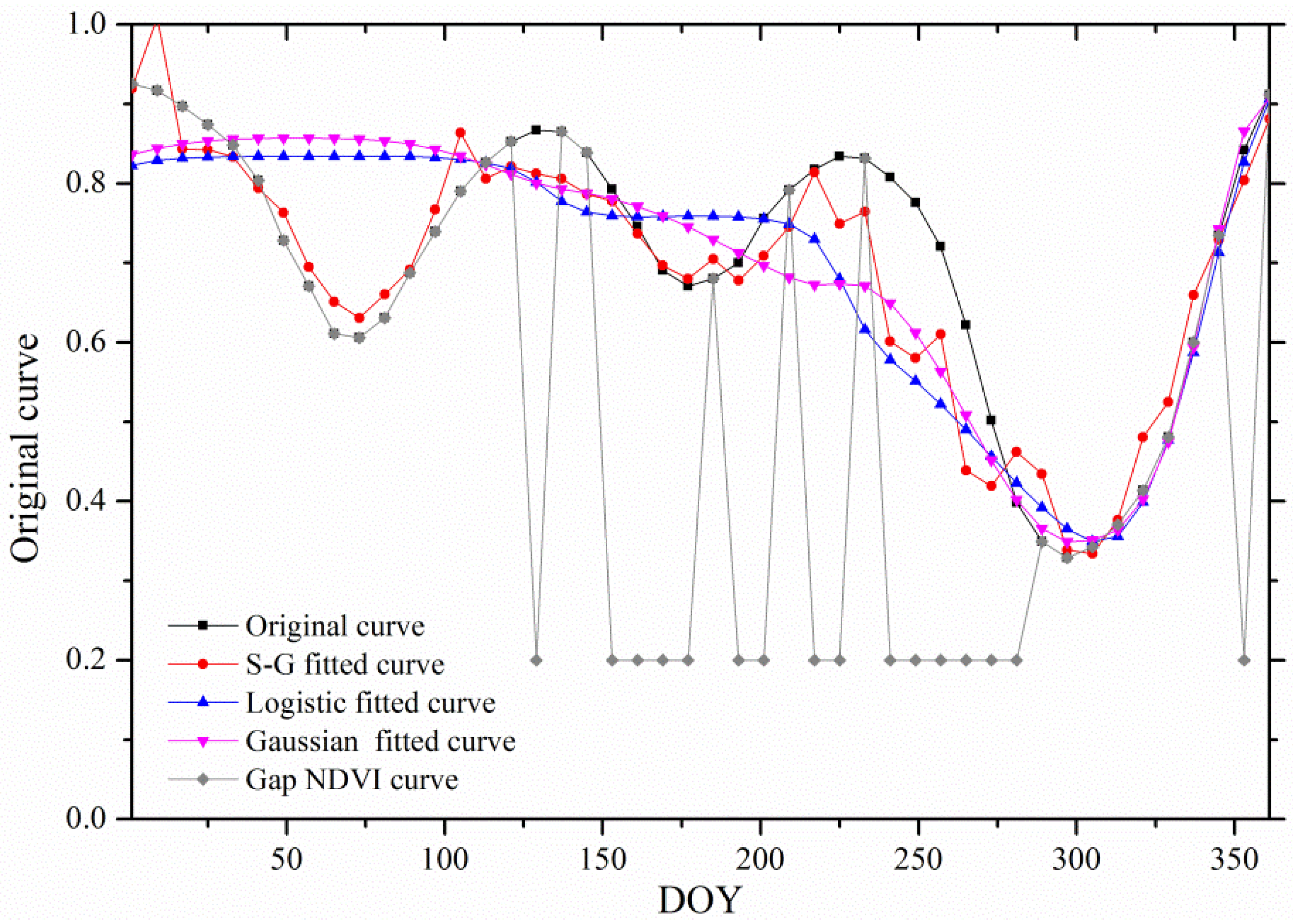
3. Data Preprocessing

Even after being corrected, the effects of the BRDF (Bidirectional Reflectance Distribution Function), clouds, ozone, dust, and other aerosols generally decreased the near infrared reflectance and affected the VI time series in the form of noise. In particular, due to the cloudy and rainy climate characteristic sf Vietnam, cloud cover seriously affects the quality of the NDVI time series, especially during the monsoon season. We used the internal cloud algorithm flag to calculate the possibility of cloud appearance in Vietnam [48]. As shown in Figure 1, among the 46 MODIS images, the cloud coverage of 33 MODIS images exceeded 20%, and that of 16 images exceeded 40%. During the monsoon season of Vietnam (May to November, namely, days 120 to days 304), the mean cloud coverage was 47%. Thus, we first de-noised the NDVI time series to reduce the influence of the atmosphere.
Various noise reduction methods have been adapted to temporal NDVI data reconstruction [49,50,51,52,53]. Hird and McDermid [54] advised caution in the application of noise reduction techniques and also argued that the strength and nature of the noise present in a dataset should be considered when selecting a method for NDVI time-series reconstruction. We manually created some NDVI time series with cloud gaps from a clear sky rice growth NDVI time series and using three noise reduction methods (the adaptive Savizky–Golay filter, the Asymmetric Gaussian function, and the Double logistic function) in the TIMESAT software [55] to reconstruct the gap NDVI time series with consideration of the QA data, we found that the Logistic algorithm’s overall fitting degree was the highest but that the S-G algorithm provided the best fit at the turning points caused by changes in rice phenology. However, it is difficult to produce a quantitative evaluation of the best algorithm for fitting every curve in every phase. Thus, we assessed the characteristics of each algorithm, as shown in Figure 3. The curves fitted by the Logistic and Gaussian algorithms are smooth, and the Logistic algorithm is the “smoothest” curve-fitting method. However, the curves fit by the S-G algorithm preserve more of the original NDVI values at the turning points.
Figure 3. Comparison between S-G algorithm filtering, Logistic algorithm filtering, and Gaussian algorithm filtering, where the black line denotes the original NDVI curves, which are sampled from a clear sky rice growth point; the red line denotes the S-G-algorithm-fitted NDVI curve with our manually generated gap NDVI curve; the Logistic fitted curve is denoted by the blue line; and the Gaussian-algorithm-fitted simulated gap NDVI is denoted by the green line.
Remotesensing 08 00019 g003
Finally, we reconstructed the NDVI time-series data using S-G filtering combined with the QA data. Adaptive Savizky–Golay filtering was used to replace each data value yi, i = 1,…, N with a linear combination of nearby values in a window, as shown in Equation (2):
j = n n c j y i + j
where c j is the weight of the ith NDVI value of the filter, which is replaced by the weighted QA value of the NDVI. The data value y i is replaced by the average of the values in the window. The window width n denotes the filter size and is the half-width of the smoothing window. The index j is the running index of the original ordinate data table.
During the fitting process, universal settings were applied to each algorithm, namely, the adaptation strength was equal to 4.0, the number of envelope iterations was equal to 2, and the same QA data layers were used. In addition, in the case of Savizky–Golay filtering, the size of the moving window was set to 4 [56].

4. Methods

After the NDVI time series were reconstructed via S-G filtering, we applied DTW-based NDVI time-series similarity measurements for detecting rice from time-series MODIS data. The method consists of two major procedures: (i) building a standard NDVI time-series base for rice growth cycles through field sampling data; and (ii) extracting rice fields based on the DTW distance of the standard rice-growth NDVI time-series data. The DTW distance was applied to sequences of NDVI values of every pixel. Each pixel had two attributes, namely, its coordinates (x, y) and an NDVI sequence defined as < NDVI1, NDVI2,…, NDVIn>. Then, a sequence was identified as <NDVI1(x, y), NDVI2(x, y),…, NDVIn(x, y)>. Because the MOD09A1 annual period includes 46 images, n equals 46. We then calculated the DTW distance of the sequence with the standard rice growth NDVI time series of each region, and a DTW distance was calculated for each pixel with the standard rice growth NDVI time series, thereby determining the similarity of each pixel’s NDVI time series with the standard rice growth NDVI time series. Using this similarity measure, we distinguished the rice from other crops.

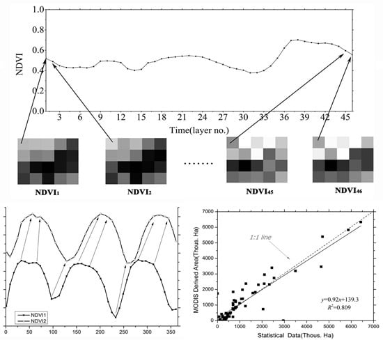
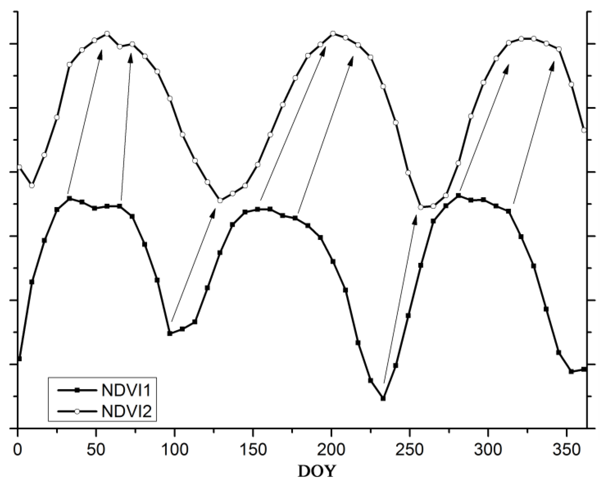
4.1. Building Standard NDVI Time-Series Base

After the NDVI data were subjected to noise filtering, we combined the 98 long-term-cultivated pure rice field points obtained from field survey data with the 268 pure rice field points obtained from Google-Earth-selected rice field points (a total of 366 points) and composed a standard rice growth NDVI time-series base as a reference NDVI time series. Among the 366 sampled rice field points, 92 were located in the North Central Coast, 86 in the Mekong River Delta, 67 in the South Central Coast, 41 in the Red River delta, 33 in the Central Highlands, 27 in the South East, 21 in the North East, and 20 in the North West. We averaged the NDVI time series with similar shapes and obtained a typical NDVI curve for each region. In addition, we used the same standard rice growth NDVI time series for the South Central Coast, Central Highlands, and South East regions because of the similar terrain, light, and temperature conditions characterizing these regions. Because the field survey data included 53 points containing information about the irrigation system of the rice growth points, we indicated the single, double, and triple rice by the shape of the NDVI time series of these 53 rice growth points. The Google-Earth-selected rice field points do not include information about the irrigation system in Vietnam, and we judged the rice cropping situation based on the shapes of curves, similar to the 53 NDVI time-series points from the field-collected information.

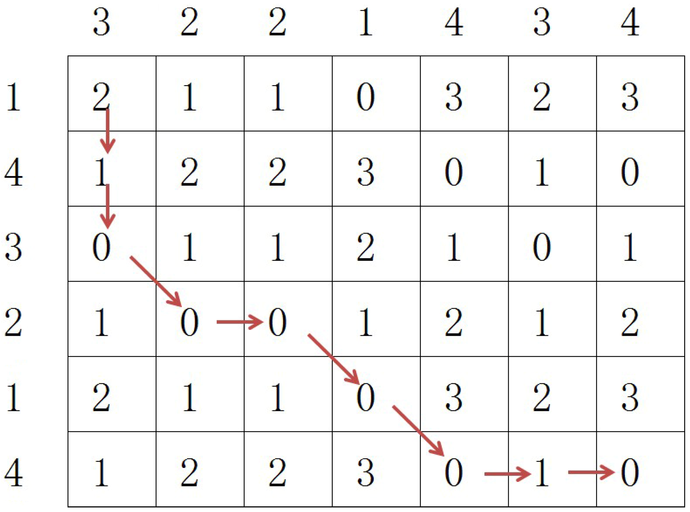
4.2. Dynamic Time Warping Based on Time-Series Similarity Measurements

DTW uses a dynamic programming technique to find the minimal distance between two time series, where sequences are warped by stretching or shrinking the time dimension [57]. The DTW algorithm is described below.
Suppose that we have two time series, i.e., C = {c1,c2,…,cm} and Q = {q1,q2,…,qn}, with respective lengths of m and n. We construct an m × n matrix Am × n and define the distance between each element as aij = d(Ci,Qj) = ( C i Q j ) 2 . In the matrix Am × n, a winding path is set by a group of adjacent matrix elements, and notes for W = {w1, w2,..., wk} and the kth element in W are defined as wk = (aij)k; this path must satisfy the following conditions:
  • Monotonicity constraint: wk = aij, wk+1 = ai’j’, then i’ ≥ i and j’ ≥ j
  • Endpoint constraint: w1 = a11, wk = amn
  • Continuity constraint: wk = aij, wk+1 = ai’j’; then i’ ≤ i + 1 and j’ ≤ j + 1.
This element must satisfy the condition 0 ≤ i − i’, 0 ≤ j − j’ ≤ 1, and thus, DTW (C,Q) = min ( 1 K i = 1 K W i ) . The DTW algorithm can be summarized by applying ideal dynamic programming to find the best (i.e., least bending) cost path, as shown in Equation (3):
{ D ( 1 , 1 ) = a 11 , D ( i , j ) = a i j + min { D ( i 1 , j 1 ) , D ( i , j 1 ) D ( i 1 , j ) }
where i = 2,3,…,m and represents the Row index of the matrix and j = 2,3,…n and represents the Column index of the matrix. D (i, j) is the minimum cumulative value of the winding paths.
Take the following two sequences as an example: sequences C = {3, 2, 2, 1, 4, 3, 4} and Q = {1, 4, 3, 2, 1, 4}. The matrixes of C and Q are given in Figure 4. The DTW distance between sequences C and Q is 2 + 1 + 0 + 0 + 0 + 0 + 0 + 1 + 0 = 4.
Figure 4. Example of DTW distance. The distance between each element of sequence C = {3, 2, 2, 1, 4, 3, 4} and sequence Q = {1, 4, 3, 2, 1, 4} is used to build a matrix, and the DTW uses a dynamic programming technique to find the minimal distance between two time series. The DTW distance is 2 + 1 + 0 + 0 + 0 + 0 + 0 + 1 + 0 = 4.
Remotesensing 08 00019 g004
In this paper, C refers to NDVI time series in the standard profile (constructed NDVI time-series base), and Q refers to the NDVI time series of the pixel. ci and qj denote the absolute value of the NDVI value in the NDVI time series. In Vietnam, the crop phenological stages are not fixed, and the planting dates depend on rainfall conditions. The planting date for irrigated rice exhibits greater variance, and geographical factors extend the variance of the length of each phenological stage. Thus, the absolute value between the NDVI time series of rice growth pixels may differ from the reference NDVI time series. As Figure 5 illustrates, suppose that NDVI1 is the reference NDVI time series and that NDVI2 is the NDVI time series of a pixel. Because the rice planting data for the pixels correspond to dates after those of the rice planting data of the reference NDVI time series, the phases are not aligned with the reference data; however, the DTW algorithm aligns the phases between these two NDVI time series by stretching or shrinking the time dimension. As a result, the DTW distance similarity measure allows for the identification of similar rice types despite dislocations of the NDVI time series because the DTW distance is small, and when applying a proper threshold to the DTW distance, they are the same type.
Figure 5. Illustration of DTW-corrected distances. The NDVI2 cycle’s planting date is later than that of the NDVI1 cycle.
Remotesensing 08 00019 g005

5. Results

5.1. Standard NDVI Time-Series Base and DTW Distance

For the purpose of getting standard rice growth NDVI time-series, we acquired 366 rice field points and composed a standard rice growth NDVI time-series base as the reference NDVI time series. Among the 366 sampled rice field points, a total of 92 sampled rice field points were located in the North Central Coast, 86 in the Mekong River Delta, 67 in the South Central Coast, 41 in the Red River delta, 33 in the Central Highlands, 27 in the South East, 21 in the North East, and 20 in the North West. NDVI time-series with similar shapes were combined and averaged (average NDVI at each layer to get a new NDVI time-series) to obtain the typical NDVI curves for each region. The standard rice growth NDVI time-series of each region is shown in Table 1.
Table 1. Standard rice growing NDVI time series and calculated DTW distance.
RegionTime Series ShapeTime Series ShapeTime Series Shape
North East & Red River Delta Remotesensing 08 00019 i001
Irrigated Double Rice Cropping in North East region
Remotesensing 08 00019 i002
Irrigated Double Rice Cropping in Red River Delta
North West Remotesensing 08 00019 i003
Rain-fed Single Rice Cropping
Remotesensing 08 00019 i004
Irrigated Double Rice Cropping
North Central Coast Remotesensing 08 00019 i005
Irrigated Double Rice Cropping
Remotesensing 08 00019 i006
Irrigated Single Rice Cropping I
Remotesensing 08 00019 i007
Rain-fed Single Rice Cropping
South Central Coast, Central Highlands & South East Remotesensing 08 00019 i008
Irrigated Double Rice Cropping
Remotesensing 08 00019 i009
Irrigated Triple Rice Cropping
Remotesensing 08 00019 i010
Rain-fed Single Rice Cropping
Mekong River Delta Remotesensing 08 00019 i011
Irrigated Triple Rice Cropping I
Remotesensing 08 00019 i012
Irrigated Double Rice Cropping I
Remotesensing 08 00019 i013
Irrigated Single Rice Cropping
Remotesensing 08 00019 i014
Irrigated Double Rice Cropping II
Remotesensing 08 00019 i015
Irrigated Triple Rice Cropping II
Remotesensing 08 00019 i016
Irrigated Triple Rice Cropping III
After obtaining the standard NDVI time series, we calculated the DTW distance between the NDVI time-series of every pixel to the standard NDVI cycle at different regions, as shown in Figure 6. It is acknowledged in the DTW algorithm that the NDVI cycle shapes exhibit greater similarity if the DTW distances are shorter. To keep this paper reasonably concise, we demonstrate six DTW distances of NDVI time series for the Mekong River Delta. The six types of rice growth NDVI time series for the Mekong River Delta in Table 1 correspond to the six maps of DTW distances shown in Figure 6. The calculation is performed in MATLAB using a loop statement.
Figure 6a shows that the DTW distances for the irrigated single rice NDVI time series are large in the wild region in the southern region of the Mekong River Delta, which denotes the dissimilarity between the NDVI time series of the pixels with the standard NDVI time series of the irrigated single rice. At the river mouth and southern region, the similarity between pixels with irrigated single rice is relatively high because the DTW distance is small. Figure 6b,c show the DTW distance with the irrigated double rice cropping I. Note that the similarity is high in certain regions in the middle north region; however, in Figure 6f (DTW distance with triple rice cropping III), the DTW distances are smaller, and thus the large regions in this area are growing triple rice.
Figure 6. The results for the DTW distance: (a) The DTW distance of single rice cropping in the Mekong River Delta; (b) the DTW distance of double rice cropping I in the Mekong River Delta; (c) the DTW distance of double rice cropping II in the Mekong River Delta; (d) the DTW distance of triple rice cropping I in the Mekong River Delta; (e) the DTW distance of triple rice cropping II in the Mekong River Delta; (f) the DTW distance of triple rice cropping III in the Mekong River Delta.
Remotesensing 08 00019 g006aRemotesensing 08 00019 g006bRemotesensing 08 00019 g006c

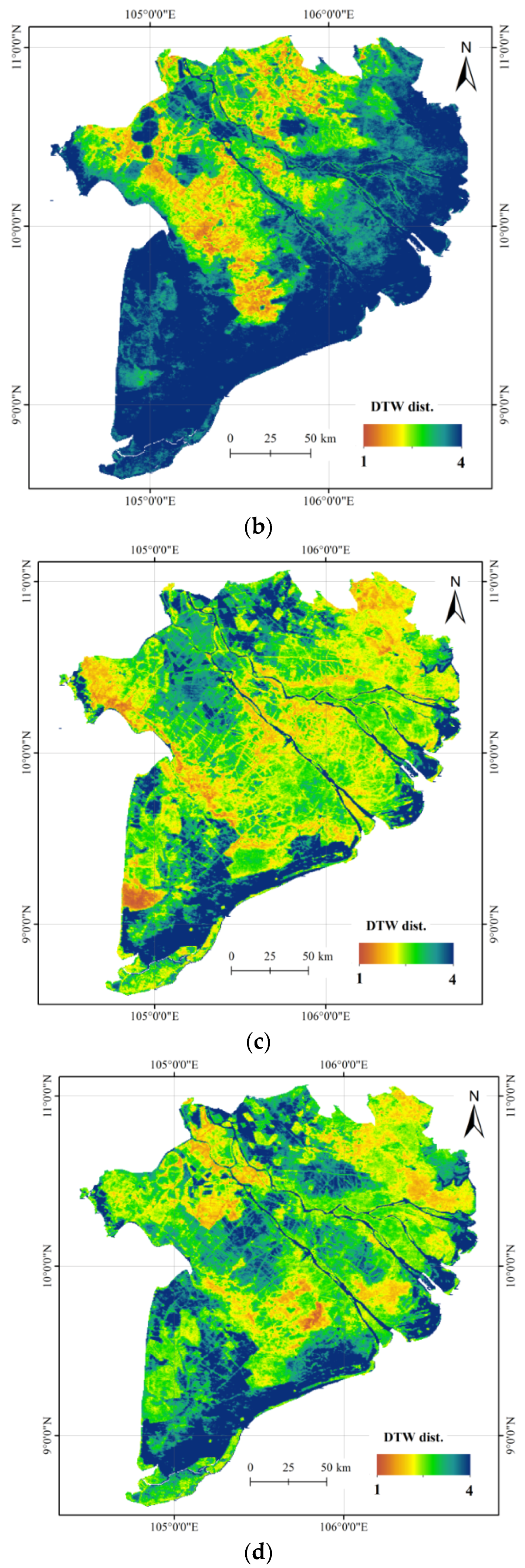
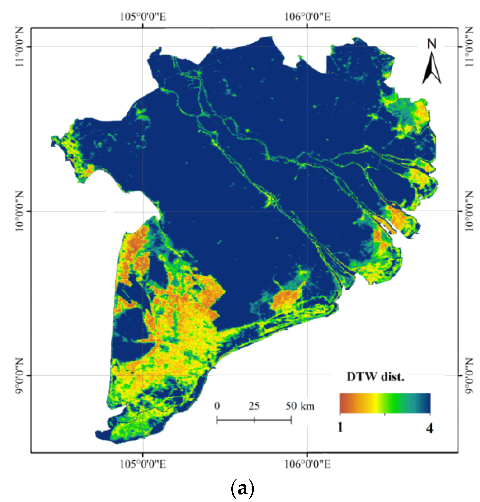
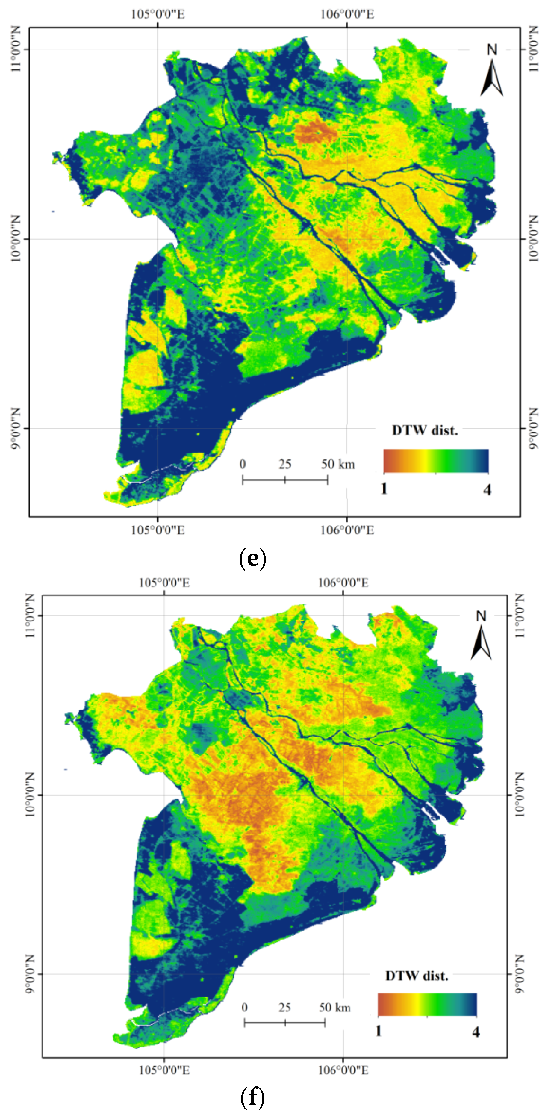
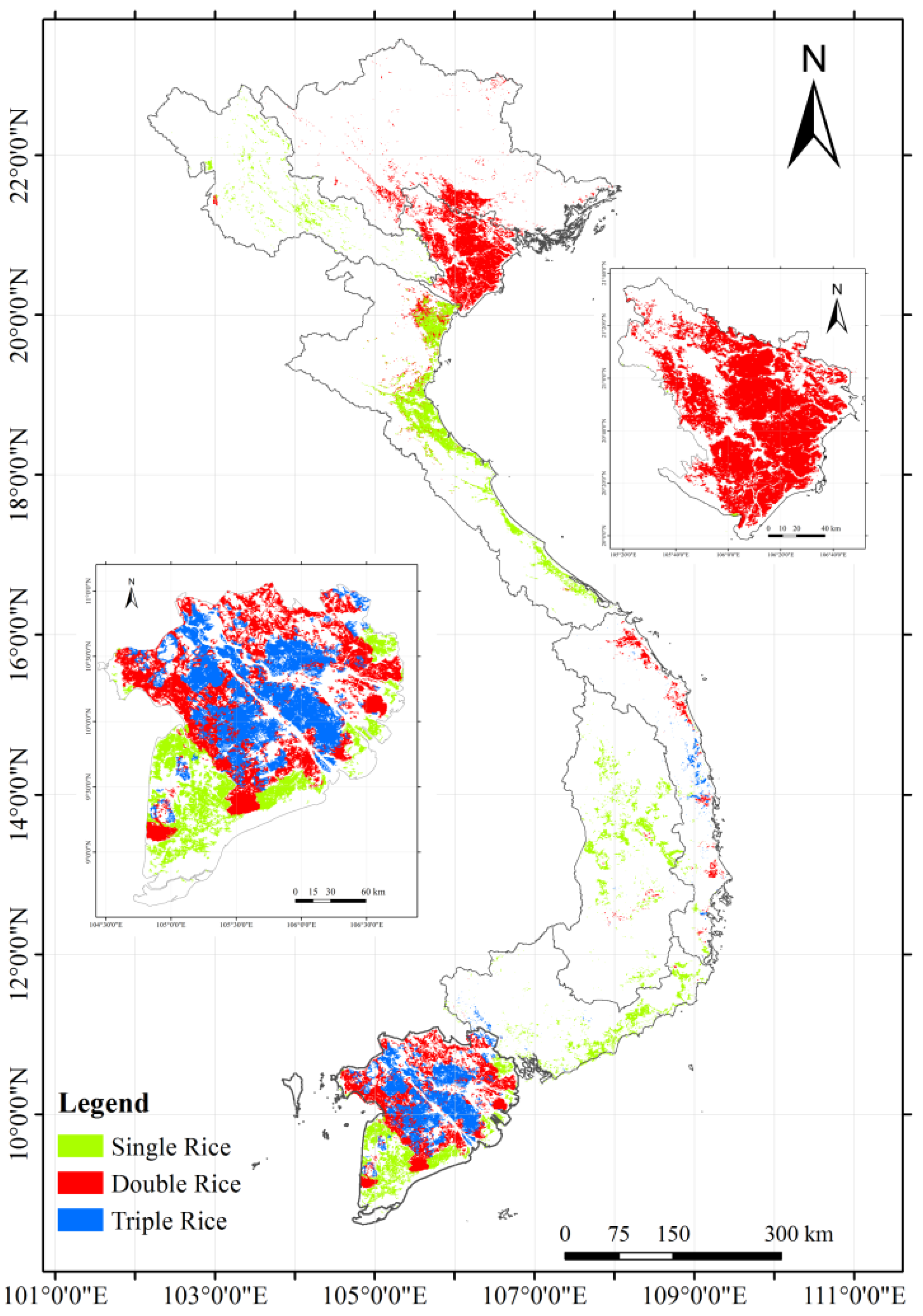
5.2. DTW Threshold and Rice Distribution Map

The DTW distance can reflect the degree of similarity as well as dissimilarity of the standard rice growth NDVI time-series with the pixels’ NDVI time-series. It is acknowledged in the DTW algorithm that the NDVI cycle shapes exhibit greater similarity if the DTW distances are shorter. We perform an interactive examination of the NDVI time series and ground-truth data to determine the cut-off DTW distance thresholds to identify single-crop rice and multiple-crop rice. The threshold values were set as shown in Table 2. It is assumed that the pixels’ NDVI time-series’ DTW distance greater than the threshold shows in Table 2 are not likely to be a rice planted field.
Table 2. Thresholds of DTW distance applied to multi-cultivated rice in each region.
North EastNorth WestRed River DeltaNorth Central CoastSouth Central Coast, Central Highlands & South EastMekong River Delta
Single rice3.83.73.4I. 3.3 II. 3.63.53.6
Double rice3.843.43.73.6I. 3.9 II. 3.4
Triple rice3.53.5I. 3.7 II. 3.5 III. 3.2
Each pixel’s DTW distance to the standard rice-growing NDVI curve was calculated, and pixels with a DTW distance for a crop type that exceeded these thresholds were considered unlikely to be the dominant crop type across the extent of the pixel. Overlaid pixels with smaller DTW distances within the threshold value were caused by the presence of mixed pixels (for example, if the DTW distance of triple rice cropping III in Mekong River Delta for a pixel is 2.7 and if the DTW distance of triple rice cropping I in Mekong River Delta is 2.8 for the same pixel, where both values are below the threshold), and we determined the crop type based on the lowest DTW distance, namely triple rice cropping III in the Mekong River Delta. Finally, the spatial distribution of rice in Vietnam is shown in Figure 7.
The application of the DTW-based similarity measure to the NDVI time series for the Vietnam rice cropping system for 2010 produces a rice crop type map for Vietnam as shown in Figure 7. The Red River Delta and Mekong River Delta are the most intensive rice cropping regions in Vietnam, and the respective cropping intensities are approximately 105.5% and 101.6%. Because the statistical records of the rice cropping areas by province in 2010 do not discriminate plantation times during the year, we unified the statistical data with the MODIS-derived data by summing up the extracted single rice areas; if there were double rice cropping areas, we counted the area twice and added it to the single rice area, so as to obtain the triple rice cropping area. For example, in the Red River Delta, the total crop area of double rice is 7704.5 thousand ha, single rice cropping in the Red River Delta represents an area of 165 thousand ha, and the total sown area is 7704.5 × 2 + 165 = 15,574 thousand ha. The Mekong River Delta exhibits mixed types of single, double, and triple cropped rice, primarily being composed of double and triple cropped rice. The South East Coast contains single, double, and triple cropped rice. Other regions in Vietnam, including the North East, North West, North East Coast, Central Highland, and Southeast regions, are mountainous and contain mostly single cropped rice in the costal lowlands. The areas of single rice, double rice, and triple rice’s area derived by MODIS data and the statistical data are shown in Table 3.
Figure 7. Result of rice cultivation area extraction using DTW-based similarity measure.
Remotesensing 08 00019 g007

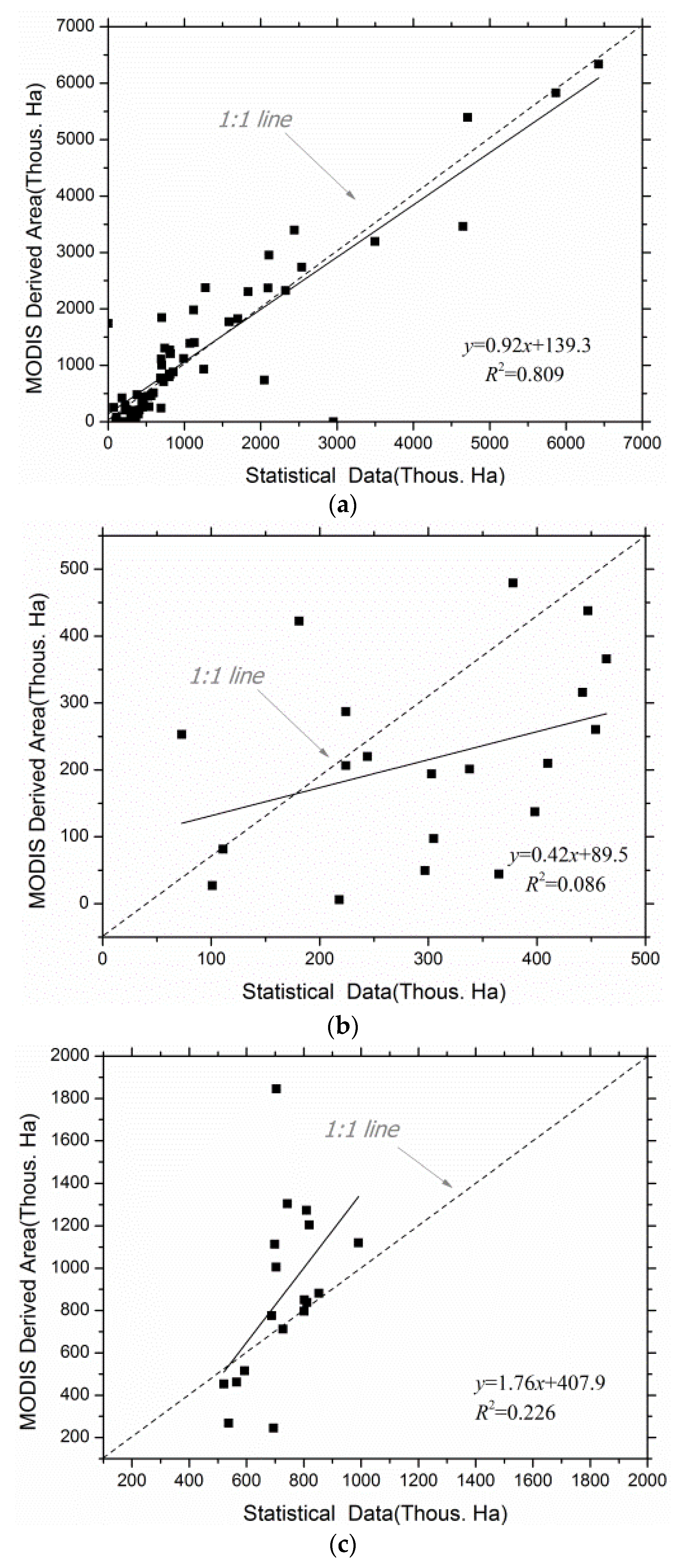
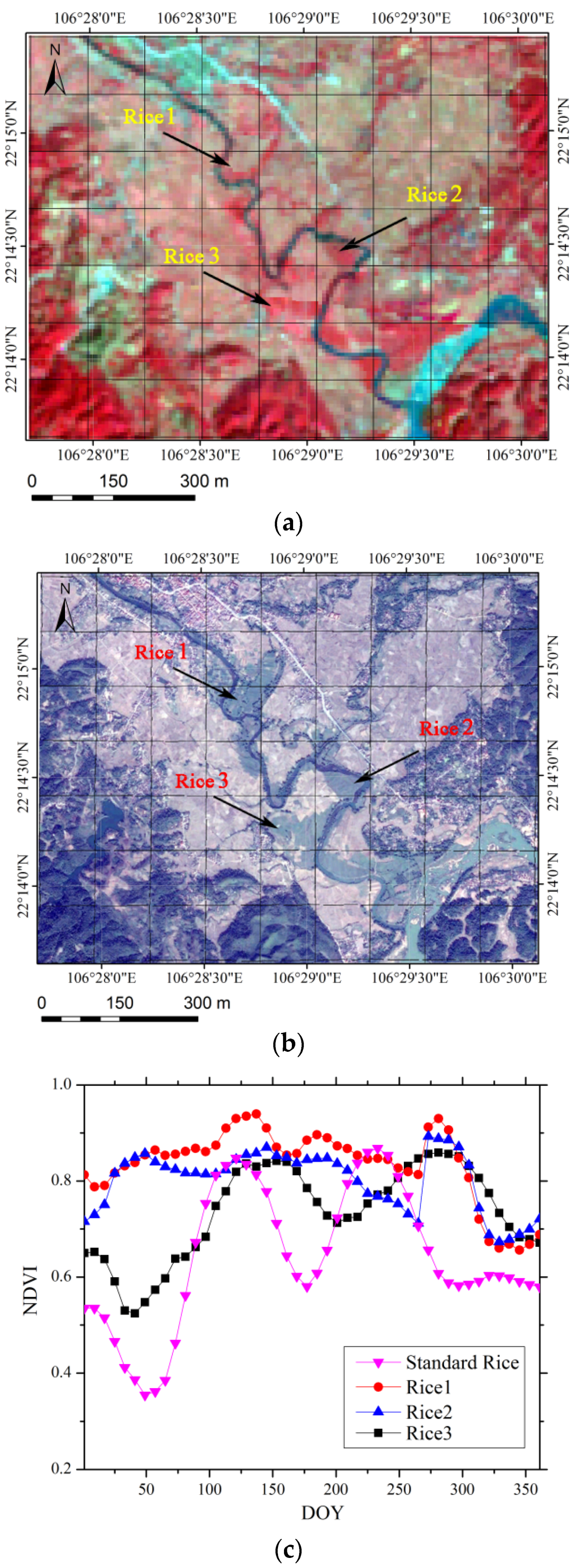
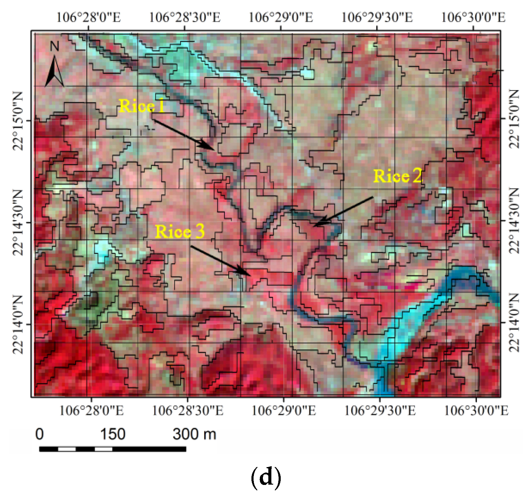
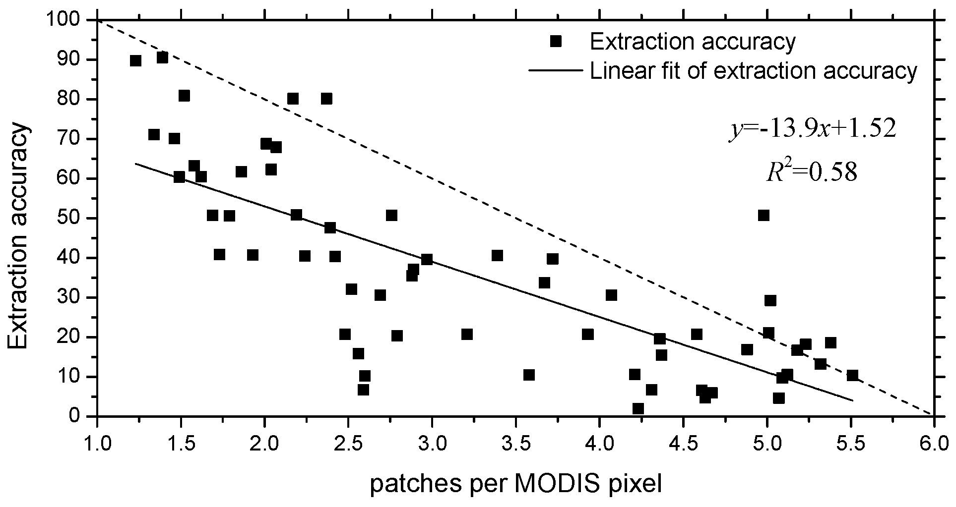
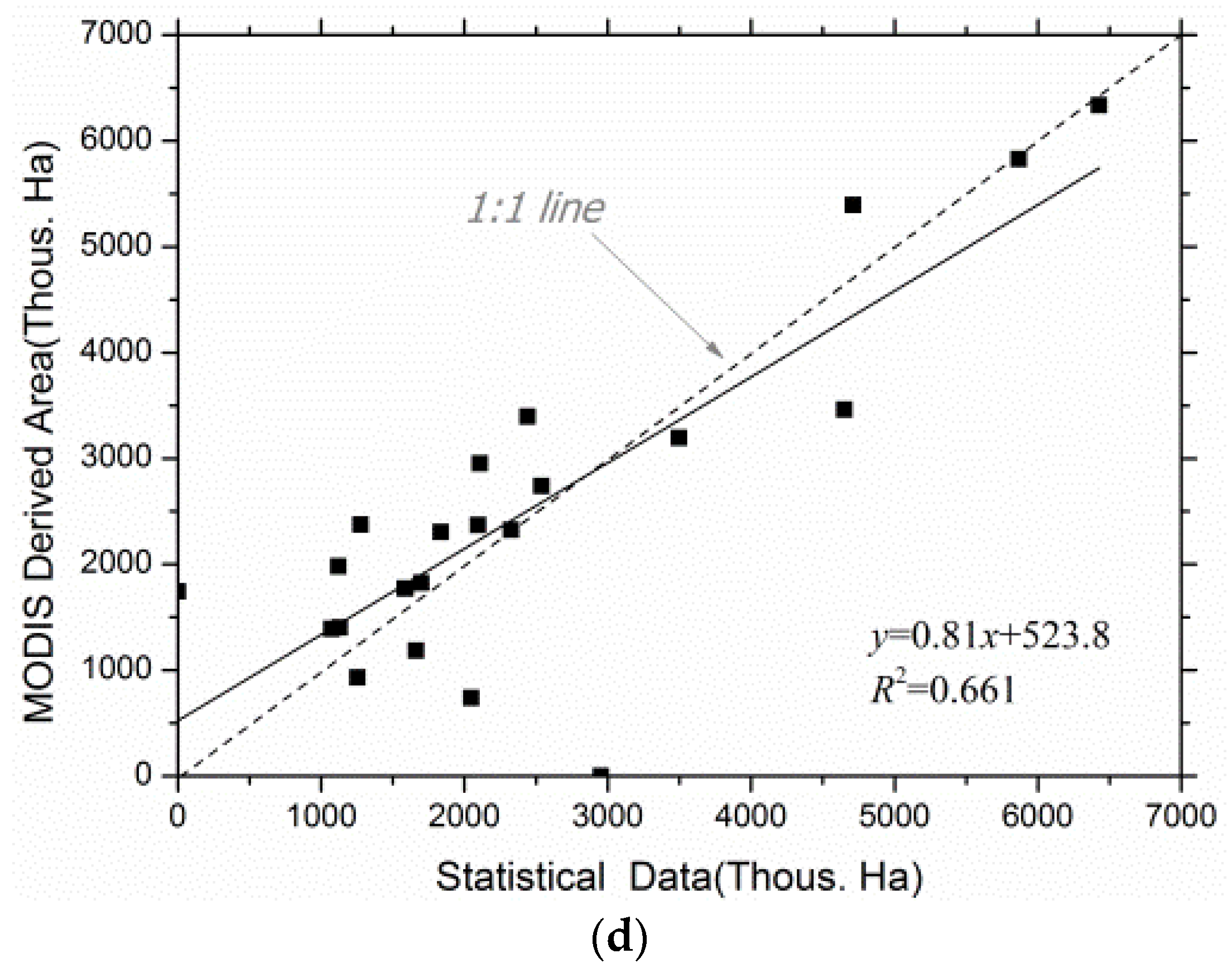
5.3. Accuracy Assessment

Figure 8 shows a comparison between the statistical data and the MODIS-derived rice areas. The statistical records of the total rice cropped areas in 2010 by province are presented. This comparison shows that at the national scale, as demonstrated in Figure 8a, the R2 value is 0.809, indicating that the two data points fit well. However, at the province scale, the results are not ideal. We separate the results into three components using the statistical data. The first component is rice-planted areas smaller than 500 km2 in the statistical data, representing 21 provinces. The second component includes rice-planted areas from 500 km2 to 1000 km2 in the statistical data, representing 18 provinces, and the third component is the statistical rice-planted areas from 1000 km2 to 7000 km2, representing 22 provinces. The comparison between the statistical data and the MODIS-derived rice areas for 21 provinces of the first component, where rice planting might be scattered or small, is shown in Figure 8b; the R2 between the two datasets in this component is 0.086, which shows that they are significantly unrelated. The comparison between the statistical data and the MODIS-derived rice areas for 18 provinces of the second component is shown in Figure 8c; the R2 of the comparison for this component is 0.226, which is greater than that in the first comparison; however, the result remains unsatisfactory. For the third component for 22 provinces where rice planting is relatively intensive, the comparison between the statistical data and the MODIS-derived rice areas is shown in Figure 8d, and the R2 between the two datasets was 0.661.
Table 3. Statistics of rice cropping areas in each province derived from MODIS.
Agriculture District/ProvinceStatistic AreaMODIS Extracted AreaAgriculture District/ProvinceStatistic AreaMODIS Extracted Area
Total AreaTotal AreaSingle RiceDouble RiceTriple RiceTotal AreaTotal AreaSingle RiceDouble RiceTriple Rice
Red River Delta11,50115,5741657704.50North East & North West66646241.81209.725160
North Central & South Central (Coastal)12,14113,205.16539.82116.8479.2South East1263697.9533.61.353.9
Central Highlands21783212.42982.3101.78.9Mekong River Delta39,45940,633.31315.58607.87367.4
Figure 8. Comparison between extraction results and the statistical data: (a) comparison of statistical data and MODIS-derived rice areas for the 63 provinces in Vietnam; (b) comparison of planted areas of less than 500 km2 for a total of 22 provinces using statistical data with the MODIS-derived rice areas; (c) comparison of statistical data of planted areas from 500 km2 to 1000 km2 for a total of 18 provinces and MODIS-derived rice areas; (d) comparison of statistical data of planted areas from 1000 km2 to 7000 km2 for a total of 23 provinces and MODIS-derived rice areas.
Remotesensing 08 00019 g008aRemotesensing 08 00019 g008b
Comparisons were also performed between the data sampled from the ground-truth data and Google Earth data and the MODIS-derived rice distribution results. In addition to the field survey points, we randomly generated 1200 points on the DEM-masked map and validated the land cover type using Google Earth high-resolution images for accuracy validation. Of the 1200 ground-truth survey data points, we obtained 365 rice field points and 835 non-rice field points. We cannot determine single, double, or triple rice fields from the Google Earth data, and the types of rice fields are not recognized; thus, we simply verified whether rice was distinguished from non-rice. Among the 365 rice field points, 191 were correctly classified as rice fields, and among the 835 non-rice field points, 127 were falsely classified as rice fields. The overall accuracy is 74.9%, the rice-field omission error is 47.7%, and the rice-field commission error is 34.8%.
To correspond to the analysis of the results of the quantity validation, we separated the provinces into three groups based on the number of rice field points. A total of 23 provinces had fewer than tw field samples, 20 provinces had between three and seven field samples, and 18 provinces had between eight and 28 field samples. The results are shown in Table 4. Although the rice plantation classification accuracy was slightly lower, the results of the provincial spatial validation corresponded well with the quantity validation results from the provinces. In the first group, the rice classification accuracy of 15.4% was not satisfactory. The second group’s classification accuracy for rice was relatively high, at 37.6%, which was also low compared to the third group. In the Discussion section, we explain the cause of the low accuracy. The last group of provinces exhibited a greater chance of accurately identifying rice plantation area, with a value of 63.5%, which is relatively high.
Table 4. Accuracy assessment of the classified rice crops based on field survey points. We separated the provinces into three groups based on the number of rice field points. The first group comprises 23 provinces with less than two field samples, the second group comprises 20 provinces with between three and seven field samples, and the third group comprises 18 provinces with between eight and 28 field samples.
No. of Field Survey PointsNo. of Correctly Classified Rice PointsNo. of Rice PointsNo. of Correctly Classified Non-Rice PointsNo. of Non-Rice PointsOverall Accuracy (%)Accuracy of Rice Classification (%)Rice Field Omission Errors (%)Rice Field Commission Errors (%)
Entire area120019136570883574.952.347.734.8
First part32442627429885.815.484.692.3
Second part3914110923728271.137.662.441.3
Third part48514623019725570.763.536.525.2
Due to the notably low extraction accuracy of the rice fields in the provinces, we examined whether the MOD09A1 data have sufficient spatial resolution to discriminate rice fields in these provinces. Figure 9 shows a fractal rice field in the North East in which rice was planted near the river. In Figure 9a, the rice cropping is scattered due to the mountainous terrain. In Figure 9c, the DTW distances of the three rice fields with standard rice field NDVI are 0.42, 0.53, and 0.57, exceeding the threshold in Table 2 so that it would not be recognized as a rice field.
Figure 9. Fractal rice field in the North East region, in which rice was planted nearby the river: (a) the Landsat TM image for 5 April 2009, in the North East region. The grid in black is the corresponding extent of a pixel in MODIS pixel.; (b) The Google Earth image obtained on 18 December 2013; (c) the NDVI curve of three points in the rice area; (d) the segmentation result based on multiresolution segmentation and the TM image.
Remotesensing 08 00019 g009aRemotesensing 08 00019 g009b
The parcel area of paddy fields is related to classification accuracy, and to evaluate the heterogeneity of land cover we performed multi-resolution segmentation (the scales of the multi-resolution segmentation are the same) inside MODIS pixels on the TM image, and in each region, one TM image in the DEM masked the map to exclude water and permanent woodland. The relationship between the land cover heterogeneity and DTW-extracted rice field accuracy is shown in Figure 10; the figure shows the decreasing trends of extraction accuracy when the number of patches per MODIS pixel is increased, which denotes a greater heterogeneity of land cover.
Figure 10. Decreasing trends of extraction accuracy when the patches per MODIS pixel are increased, which denotes a greater heterogeneity of the land cover.
Remotesensing 08 00019 g010
The extraction accuracy is computed as (Ae-As)/As, where Ae is the extracted rice area and as is the statistical rice area. The number of patches per MODIS pixel is computed as the average number of multi-resolution segmented patches of TM images in MODIS pixels. This result shows that the rice extraction accuracy of a small rice-cropping region is decreased due to the coarse spatial resolution of MOD09A1 data.

6. Conclusions

We have developed a new systematic method for detecting the area of a paddy rice system from time-series MODIS data. The method consists of three procedures: (i) filtering the time-series NDVI data using the S-G filtering; (ii) building a standard rice-growing NDVI time series base through Google earth sample points and ground-truth data; and (iii) calculating the DTW distance of the standard rice-growth NDVI time series of each pixel and using a threshold to extract the rice field area. Our method is able to discriminate between single-rice-crop and multi-rice-crop systems in Vietnam.
In the field of pattern recognition, many algorithms have been developed to compare the similarities between curves. The DTW is a classic curve-matching technique and is defined between sequences of points. We applied the classic DTW to the recognition of NDVI curve similarity for rice field recognition. Additionally, we set a simple threshold to decide whether a pixel belongs to a specific type of rice growth NDVI time series. The selection of the threshold is performed via interactive examination with the ground-truth data and Google Earth sampling data. The accuracy assessment based on statistical data at the province level and ground-truth data obtained from field surveys and Google Earth sampling shows that our method is able to discriminate between single-rice-crop and multi-rice-crop systems in Vietnam at a national scale and that the classification accuracy is satisfactory; however, at the province scale, the accuracy is decreased. Through analysis of wrongly classified rice field points, we proved that the MOD09A1 spatial resolutions were too coarse for rice field extraction in the areas in which small rice fields are predominant and in which rice planting is scattered and fragmented.
This study confirms that the DTW approach can be applied to the determination of rice cropping systems over wide connecting areas in which rice planting scheduling is flexible and rice growth periods in different phases are uncertain. We believe that this work opens the door to a number of research directions. First, one can combine the DTW with many other mature classification approaches such as nearest neighbor and neural networks to classify satellite time-series data. Second, the DTW approach provides a more rational way to calculate the similarity or dissimilarity between curves, thereby providing a method of quantifying variations in crop cultivation. However, more scientific approaches to determining thresholds should be studied. Another problem is that the DTW distance of the standard NDVI curve shapes, which exhibit smoother and lesser dynamic changes in rice growth phenology, tend to have smaller DTW distances. As a result, the discrimination between the three types of rice is vague. Therefore, normalization between the standard NDVI curves should be studied in greater detail.
At the moment, various limitations remain, including the mixed-pixel effect. As an objective and repeatable methodology, this method is sufficiently robust for addressing complex forms of rice cropping systems in Southeast Asia.

Supplementary Files

Supplementary File 1

Acknowledgments

We gratefully acknowledge the financial support of the Key Research Program of the Chinese Academy of Sciences (grant No. KZZD-EW-08), National Natural Science Foundation of China Program (grant No. 41561144012, 41471335), The International Cooperation in Science and Technology Special Project (grant No. 2013DFA91700).

Author Contributions

Chong Huang conceived the study. Xudong Guan performed the data analysis and wrote the paper. Gaohuan Liu and Qingsheng Liu supervised and provided logistical support to the research. Xuelian Meng provided feedback on the study design and modified the manuscript. All authors reviewed and approved the manuscript.

Conflicts of Interest

The authors declare no conflict of interest.

References

  1. Fairhurst, T.; Dobermann, A. Rice in the global food supply. World 2002, 502, 454, 349–511, 675. [Google Scholar]
  2. Kuenzer, C.; Knauer, K. Remote sensing of rice crop areas. Int. J. Remote Sens. 2013, 34, 2101–2139. [Google Scholar] [CrossRef]
  3. Ricepedia. The Online Authority on Rice: Rice Species. Available online: http://ricepedia.org/ (accessed on 15 March 2015).
  4. General Statistics Office of Vietnam. Statistical Yearbook of Vietnam. Available online: http://www.gso.gov.vn/ (accessed on 15 March 2015).
  5. Bouman, B.A.M. Crop modeling and remote-sensing for yield prediction. Neth. J. Agric. Sci. 1995, 43, 143–161. [Google Scholar]
  6. Thiruvengadachari, S.; Sakhtivadivel, R. Satellite Remote Sensing for Assessment of Irrigation System Performance: A Case Study in India; IWMI Research Report: Colombo, CMB, Sri Lanka, 1997. [Google Scholar]
  7. Casanova, D.; Epema, G.F.; Goudriaan, J. Monitoring rice reflectance at field level for estimating biomass and lai. Field Crop. Res. 1998, 55, 83–92. [Google Scholar] [CrossRef]
  8. Dawson, T.P.; Curran, P.J.; North, P.R.J.; Plummer, S.E. The propagation of foliar biochemical absorption features in forest canopy reflectance: A theoretical analysis. Remote Sens. Environ. 1999, 67, 147–159. [Google Scholar] [CrossRef]
  9. Chang, K.W.; Shen, Y.; Lo, J.C. Predicting rice yield using canopy reflectance measured at booting stage. Agron. J. 2005, 97, 872–878. [Google Scholar] [CrossRef]
  10. Hatfield, J.L.; Gitelson, A.A.; Schepers, J.S.; Walthall, C.L. Application of spectral remote sensing for agronomic decisions. Agron. J. 2008, 100, S117–S131. [Google Scholar] [CrossRef]
  11. Shen, S.; Yang, S.; Li, B.; Tan, B.; Li, Z.; le Toan, T. A scheme for regional rice yield estimation using ENVISAT ASAR data. Sci. China Ser. D-Earth Sci. 2009, 52, 1183–1194. [Google Scholar] [CrossRef]
  12. Fang, H.; Wu, B.; Liu, H.; Huang, X. Using NOAA AVHRR and Landsat TM to estimate rice area year-by-year. Int. J. Remote Sens. 1998, 19, 521–525. [Google Scholar] [CrossRef]
  13. Liu, J.; Liu, M.; Tian, H.; Zhuang, D.; Zhang, Z.; Zhang, W.; Tang, X.; Deng, X. Spatial and temporal patterns of China’s cropland during 1990–2000: An analysis based on Landsat-TM data. Remote Sens. Environ. 2005, 98, 442–456. [Google Scholar] [CrossRef]
  14. Turner, M.D.; Congalton, R.G. Classification of multi-temporal Spot-XS satellite data for mapping rice fields on a west African floodplain. Int. J. Remote Sens. 1998, 19, 21–41. [Google Scholar] [CrossRef]
  15. Panigrahy, S.; Sharma, S.A. Mapping of crop rotation using multi-date Indian remote sensing satellite digital data. ISPRS J. Photogramm. Remote Sens. 1997, 52, 85–91. [Google Scholar] [CrossRef]
  16. Quarmby, N.A.; Townshend, J.R.G.; Settle, J.J.; White, K.H.; Milnes, M.; Hindle, T.L.; Silleos, N. Linear mixture modelling applied to AVHRR data for crop area estimation. Int. J. Remote Sens. 1992, 13, 415–425. [Google Scholar] [CrossRef]
  17. Li, Q.Z.; Zhang, H.X.; Du, X.; Wen, N.; Tao, Q.S. County-level rice area estimation in southern China using remote sensing data. J. Appl. Remote Sens. 2014, 8. [Google Scholar] [CrossRef]
  18. Roberts, D.A. Large area mapping of land-cover change in Rondônia using multi-temporal spectral mixture analysis and decision tree classifiers. J. Geophys. Res. 2002, 107. [Google Scholar] [CrossRef]
  19. Xiao, X.; Boles, S.; Liu, J.; Zhuang, D.; Frolking, S.; Li, C.; Salas, W.; Moore, B. Mapping paddy rice agriculture in southern China using multi-temporal MODIS images. Remote Sens. Environ. 2005, 95, 480–492. [Google Scholar] [CrossRef]
  20. Xiao, X.M.; Boles, S.; Frolking, S.; Li, C.S.; Babu, J.Y.; Salas, W.; Moore, B. Mapping paddy rice agriculture in south and southeast Asia using multi-temporal MODIS images. Remote Sens. Environ. 2006, 100, 95–113. [Google Scholar] [CrossRef]
  21. Xiao, X.; Boles, S.; Frolking, S.; Salas, W.; Moore, B.; Li, C.; He, L.; Zhao, R. Observation of flooding and rice transplanting of paddy rice fields at the site to landscape scales in China using vegetation sensor data. Int. J. Remote Sens. 2002, 23, 3009–3022. [Google Scholar] [CrossRef]
  22. Gumma, M.K.; Thenkabail, P.S.; Maunahan, A.; Islam, S.; Nelson, A. Mapping seasonal rice cropland extent and area in the high cropping intensity environment of Bangladesh using MODIS 500 m data for the year 2010. ISPRS J. Photogramm. Remote Sens. 2014, 91, 98–113. [Google Scholar] [CrossRef]
  23. Chen, C.F.; Son, N.T.; Chang, L.Y. Monitoring of rice cropping intensity in the upper Mekong delta, Vietnam using time-series MODIS data. Adv. Space Res. 2012, 49, 292–301. [Google Scholar] [CrossRef]
  24. Kontgis, C.; Schneider, A.; Ozdogan, M. Mapping rice paddy extent and intensification in the Vietnamese Mekong river delta with dense time stacks of Landsat data. Remote Sens. Environ. 2015, 169, 255–269. [Google Scholar] [CrossRef]
  25. Geerken, R.; Zaitchik, B.; Evans, J.P. Classifying rangeland vegetation type and coverage from NDVI time series using Fourier filtered cycle similarity. Int. J. Remote Sens. 2005, 26, 5535–5554. [Google Scholar] [CrossRef]
  26. Keogh, E.J.; Pazzani, M.J. Derivative dynamic time warping. In Proceedings of the SIAM International Conference on Data Mining, Columbus, OH, USA, 21 June 2001; pp. 5–7.
  27. Keogh, E.; Ratanamahatana, C.A. Exact indexing of dynamic time warping. Knowl. Inf. Syst. 2005, 7, 358–386. [Google Scholar] [CrossRef]
  28. Berndt, D.J.; Clifford, J. Using Dynamic Time Warping to Find Patterns in Time Series. In Proceedings of the KDD Workshop, Seattle, WA, USA, 12 August 1994; pp. 359–370.
  29. Chen, Y.-L.; Wu, S.-Y.; Wang, Y.-C. Discovering multi-label temporal patterns in sequence databases. Inf. Sci. 2011, 181, 398–418. [Google Scholar] [CrossRef]
  30. Kim, S.-W.; Shin, M. Subsequence matching under time warping in time-series databases: Observation, optimization, and performance results. Comput. Syst. Sci. Eng. 2008, 23, 31–42. [Google Scholar] [CrossRef]
  31. Rebai, I.; BenAyed, Y. Text-to-speech synthesis system with Arabic diacritic recognition system. Comput. Speech Lang. 2015, 34, 43–60. [Google Scholar] [CrossRef]
  32. Dockstader, S.L.; Bergkessel, K.A.; Tekalp, A.M. Feature extraction for the analysis of gait and human motion. In Proceedings of the 16th International Conference on Pattern Recognition, Quebec, QC, Canada, 15 August 2002; pp. 5–8.
  33. Lee, A.J.T.; Chen, Y.-A.; Ip, W.-C. Mining frequent trajectory patterns in spatial-temporal databases. Inf. Sci. 2009, 179, 2218–2231. [Google Scholar] [CrossRef]
  34. Niennattrakul, V.; Srisai, D.; Ratanamahatana, C.A. Shape-based template matching for time series data. Knowl. Based Syst. 2012, 26, 1–8. [Google Scholar] [CrossRef]
  35. Petitjean, F.; Ketterlin, A.; Gançarski, P. A global averaging method for dynamic time warping, with applications to clustering. Pattern Recognit. 2011, 44, 678–693. [Google Scholar] [CrossRef]
  36. Petitjean, F.; Inglada, J.; Gancarski, P. Satellite image time series analysis under time warping. IEEE Trans. Geosci. Remote Sens. 2012, 50, 3081–3095. [Google Scholar] [CrossRef]
  37. Izakian, H.; Pedrycz, W.; Jamal, I. Fuzzy clustering of time series data using dynamic time warping distance. Eng. Appl. Artif. Intell. 2015, 39, 235–244. [Google Scholar] [CrossRef]
  38. Jeong, Y.S.; Jayaraman, R. Support vector-based algorithms with weighted dynamic time warping kernel function for time series classification. Knowl. Based Syst. 2015, 75, 184–191. [Google Scholar] [CrossRef]
  39. Maclean, J.L.; Dawe, D.C.; Hardy, B.; Hettel, G.P. Rice Almanac: Source Book for the Most Important Economic Activity on Earth, 2nd ed.; CABI Publishing: Wallingford, Oxon, UK, 2002; pp. 102–105. [Google Scholar]
  40. Toshihiro, S.; Cao, V. P.; Aikihiko, K.; Khang, D.N.; Masayuki, Y. Analysis of rapid expansion of inland aquaculture and triple rice-cropping areas in a coastal area of the Vietnamese Mekong Delta using MODIS time-series imagery. Landscape Urban Plan. 2009, 92, 34–46. [Google Scholar]
  41. Son, N.-T.; Chen, C.-F.; Chen, C.-R.; Duc, H.-N.; Chang, L.-Y. A phenology-based classification of time-series MODIS data for rice crop monitoring in Mekong delta, Vietnam. Remote Sens. 2013, 6, 135–156. [Google Scholar] [CrossRef]
  42. Greg, E. LAADS Web. Available online: http://ladsweb.nascom.nasa.gov/ (accessed on 25 December 2015).
  43. U.S. Department of the Interior; U.S. Geological Survey. MOD09A1|LP DAAC: NASA Land Data Products and Services. Available online: http://lpdaac.usgs.gov/dataset_discovery/modis/modis_products_table/mod09a1/ (accessed on 25 December 2015).
  44. Huete, A.; Didan, K.; Miura, T.; Rodriguez, E.P.; Gao, X.; Ferreira, L.G. Overview of the radiometric and biophysical performance of the MODIS vegetation indices. Remote Sens. Environ. 2002, 83, 195–213. [Google Scholar] [CrossRef]
  45. Lhermitte, S.; Verbesselt, J.; Verstraeten, W.W.; Coppin, P. A comparison of time series similarity measures for classification and change detection of ecosystem dynamics. Remote Sens. Environ. 2011, 115, 3129–3152. [Google Scholar] [CrossRef]
  46. CGIAR-CSI SRTM 90m DEM Digital Elevation Database. Available online: http://srtm.csi.cgiar.org/ (accessed on 25 December 2015).
  47. Statistical Documentation and Service Centre—General Statistics Office of Vietnam. Available online: http://www.gso.gov.vn/ (accessed on 25 December 2015).
  48. Leinenkugel, P.; Kuenzer, C.; Dech, S. Comparison and enhancement of MODIS cloud mask products for Southeast Asia. Int. J. Remote Sens. 2013, 34, 2730–2748. [Google Scholar] [CrossRef]
  49. Viovy, N.; Arino, O.; Belward, A.S. The best index slope extraction (BISE)—A method for reducing noise in NDVI time-series. Int. J. Remote Sens. 1992, 13, 1585–1590. [Google Scholar] [CrossRef]
  50. Ma, M.; Veroustraete, F. Reconstructing pathfinder AVHRR land NDVI time-series data for the northwest of China. Adv. Space Res. 2006, 37, 835–840. [Google Scholar] [CrossRef]
  51. Gu, J.; Li, X.; Huang, C.; Okin, G.S. A simplified data assimilation method for reconstructing time-series MODIS NDVI data. Adv. Space Res. 2009, 44, 501–509. [Google Scholar] [CrossRef]
  52. Huang, N.E.; Shen, Z.; Long, S.R.; Wu, M.C.; Shih, H.H.; Zheng, Q.; Yen, N.C.; Tung, C.C.; Liu, H.H. The Empirical Mode Decomposition and the Hilbert Spectrum for Nonlinear and Non-Stationary Time Series Analysis. In Proceedings of the Royal Society of London A: Mathematical, Physical and Engineering Sciences, London, UK, 8 March 1998; The Royal Society: London, UK, 1998; pp. 903–995. [Google Scholar]
  53. Sakamoto, T.; Yokozawa, M.; Toritani, H.; Shibayama, M.; Ishitsuka, N.; Ohno, H. A crop phenology detection method using time-series MODIS data. Remote Sens. Environ. 2005, 96, 366–374. [Google Scholar] [CrossRef]
  54. Hird, J.N.; McDermid, G.J. Noise reduction of NDVI time series: An empirical comparison of selected techniques. Remote Sens. Environ. 2009, 113, 248–258. [Google Scholar] [CrossRef]
  55. Jonsson, P.; Eklundh, L. Seasonality extraction by function fitting to time-series of satellite sensor data. IEEE Trans. Geosci. Remote Sens. 2002, 40, 1824–1832. [Google Scholar] [CrossRef]
  56. Chen, J.; Jonsson, P.; Tamura, M.; Gu, Z.H.; Matsushita, B.; Eklundh, L. A simple method for reconstructing a high-quality NDVI time-series data set based on the Savitzky-Golay filter. Remote Sens. Environ. 2004, 91, 332–344. [Google Scholar] [CrossRef]
  57. Jeong, Y.S.; Jeong, M.K.; Omitaomu, O.A. Weighted dynamic time warping for time series classification. Pattern Recognit. 2011, 44, 2231–2240. [Google Scholar] [CrossRef]

