Estimating Horizontal Displacement between DEMs by Means of Particle Image Velocimetry Techniques

Abstract

To date, digital terrain model (DTM) accuracy has been studied almost exclusively by computing its height variable. However, the largely ignored horizontal component bears a great influence on the positional accuracy of certain linear features, e.g., in hydrological features. In an effort to fill this gap, we propose a means of measurement different from the geomatic approach, involving fluid mechanics (water and air flows) or aerodynamics. The particle image velocimetry (PIV) algorithm is proposed as an estimator of horizontal differences between digital elevation models (DEM) in grid format. After applying a scale factor to the displacement estimated by the PIV algorithm, the mean error predicted is around one-seventh of the cell size of the DEM with the greatest spatial resolution, and around one-nineteenth of the cell size of the DEM with the least spatial resolution. Our methodology allows all kinds of DTMs to be compared once they are transformed into DEM format, while also allowing comparison of data from diverse capture methods, i.e., LiDAR versus photogrammetric data sources.

1. Introduction

A lot of geomatic applications use DTMs as the basis to derive other products such as cartography, hydrological features, engineering solutions, urban planning, environmental studies, time series analyses, reports, statistics, etc. The precision and accuracy of DTMs, required for deriving the above-mentioned products, however, may vary substantially. The data capture methodology is one key to explain the precision and accuracy of DTMs and how they influence the derived product. There is a need for reliable measures of accuracy allowing comparative evaluations of DTMs from different sources, e.g., LiDAR versus photogrammetry. Most studies thus far focus on the height variable [1,2]. As the easiest variable to statistically compute and interpret, such studies focus on vertical accuracy. Some authors [3,4] studied the DEM accuracy as a function of some features (topographic index, hydrological objects). There are no reports to date of horizontal accuracy of DTMs or DEMs linked with the derived features, most likely because any such measure, if it exists, would hardly be applicable to other features [5]. More recently, algorithms were defined to link the differences between horizontal accuracy and the derived parameters of features; such algorithms could be based on a triangulated irregular network (TIN) [6,7] or DEM grid models [8]. The first approach generalizes the separation between homologous contours as the measure of horizontal discrepancy for the whole DEM, whereas the second compares several cells in two or more DEMs to estimate the horizontal discrepancy.

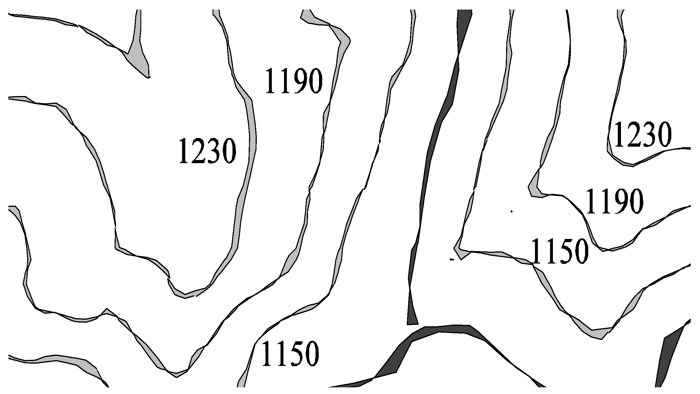
We can define the vertical accuracy for a DEM (grid structure composed of rows and columns) as the magnitude indicating how close the height of a point is, located by its horizontal position (row and column), on a DEM with respect its true value. If we have a reference DEM (RefDEM) as the ground truth we could estimate the vertical accuracy from any other DEM (CompDEM) just by computing the differences between the corresponding cell’s height from both DEMs. The vertical accuracy can be seen as the matrix: accMat = RefDEM − ComDEM. Horizontal accuracy is a little bit more complicated to understand because it may be difficult, given a point (RefP) on a RefDEM, to find its homologous point (HomP) on a CompDEM, except, for example, when RefP and HomP are a building corner, but that is not usually the case. We could understand the horizontal accuracy of a CompDEM with respect to its RefDEM; imagining the case where the CompDEM is identical to the RefDEM, then their contours would be the same. However, if we move the identical CompDEM horizontally, then the homologous contours from the CompDEM and RefDEM would not match and the discrepancy between the homologous contours indicates the horizontal discrepancy, which, consequently, is a measure of the horizontal accuracy. It is possible for each cell in the CompDEM to be horizontally displaced in any direction, so that homologous contours cross each other as shown in Figure 1, where the area between homologous contours has been filled with gray color.

Figure 1. Homologous contours (coming from homologous DEM: RefDEM and CompDEM) crossing each other and filling the area with gray color. The black color is a river piece.

Figure 1. Homologous contours (coming from homologous DEM: RefDEM and CompDEM) crossing each other and filling the area with gray color. The black color is a river piece.

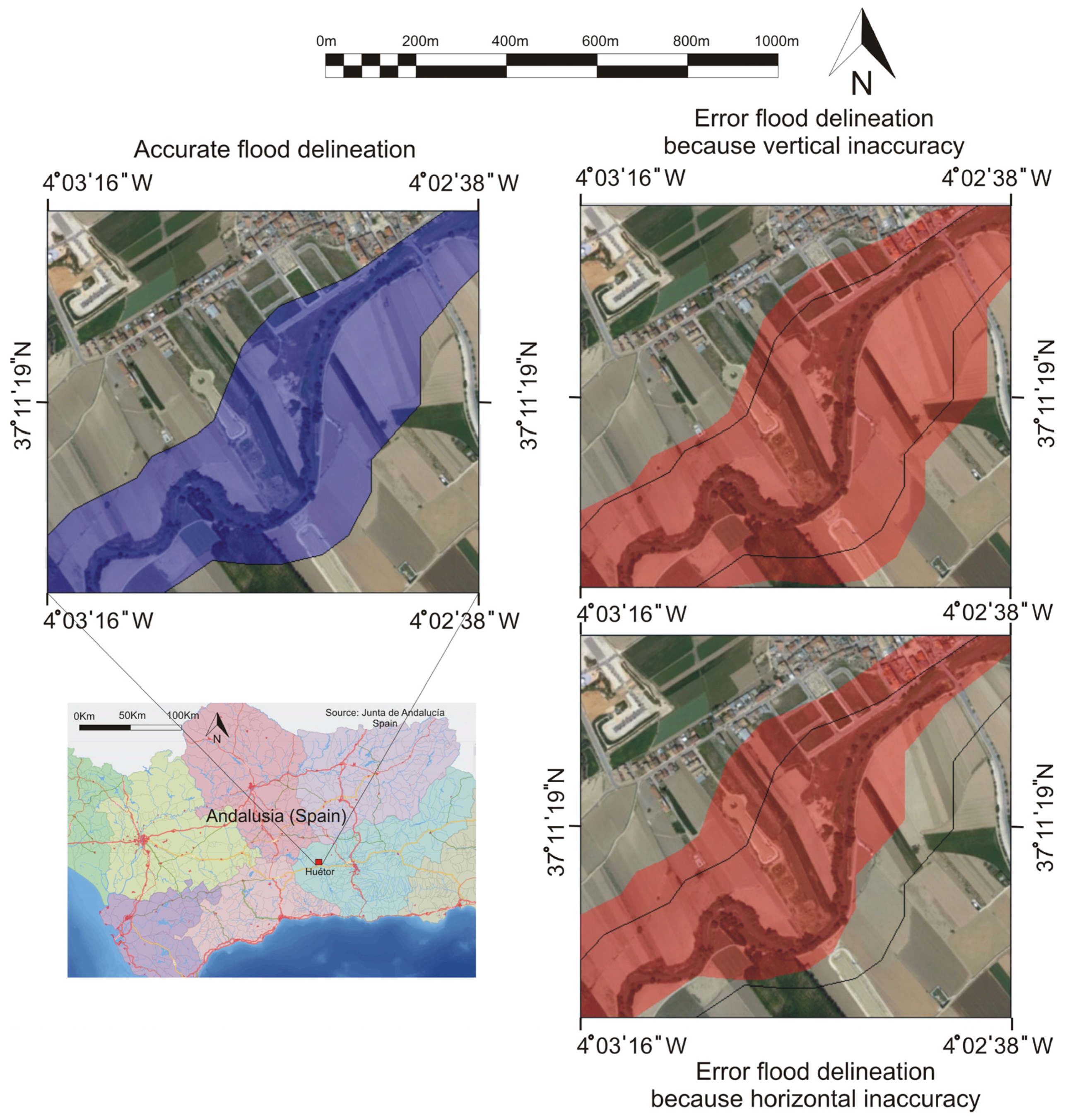
Both vertical and horizontal accuracy are important features to keep in every DEM because error in vertical and horizontal positioning could have bad consequences when, for example, computing flood risk areas. If we miscompute flood areas as a consequence of inaccurate DEMs, it would be possible to authorize, by error, the construction of some houses in flood risk areas. An illustration for both errors (vertical and horizontal inaccuracy) is shown in Figure 2: on the left the real flood area has been computed, and the image on the upper right shows an error due to vertical inaccuracy (the CompDEM altitude is higher than the RefDEM altitude and an urban area is flooded); the image on the bottom right shows the error due to horizontal inaccuracy (the CompRef is moved to the left and up direction and an urban area is flooded). Another example of horizontal accuracy importance comes from the ability of LiDAR data to produce a highly detailed drainage network [9] and it would be interesting to know the variation in the streams if computed with different DEM sources.

Landslide is another field where horizontal displacement has to be computed. There are several approaches to get such calculations, and one of them is based on series of images taken in different epochs, e.g., [10,11]. Those studies base their computation on minimizing a correlation function between a local window in the reference image and its homologous window in the compared image, according to the method explained by [12].

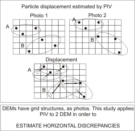
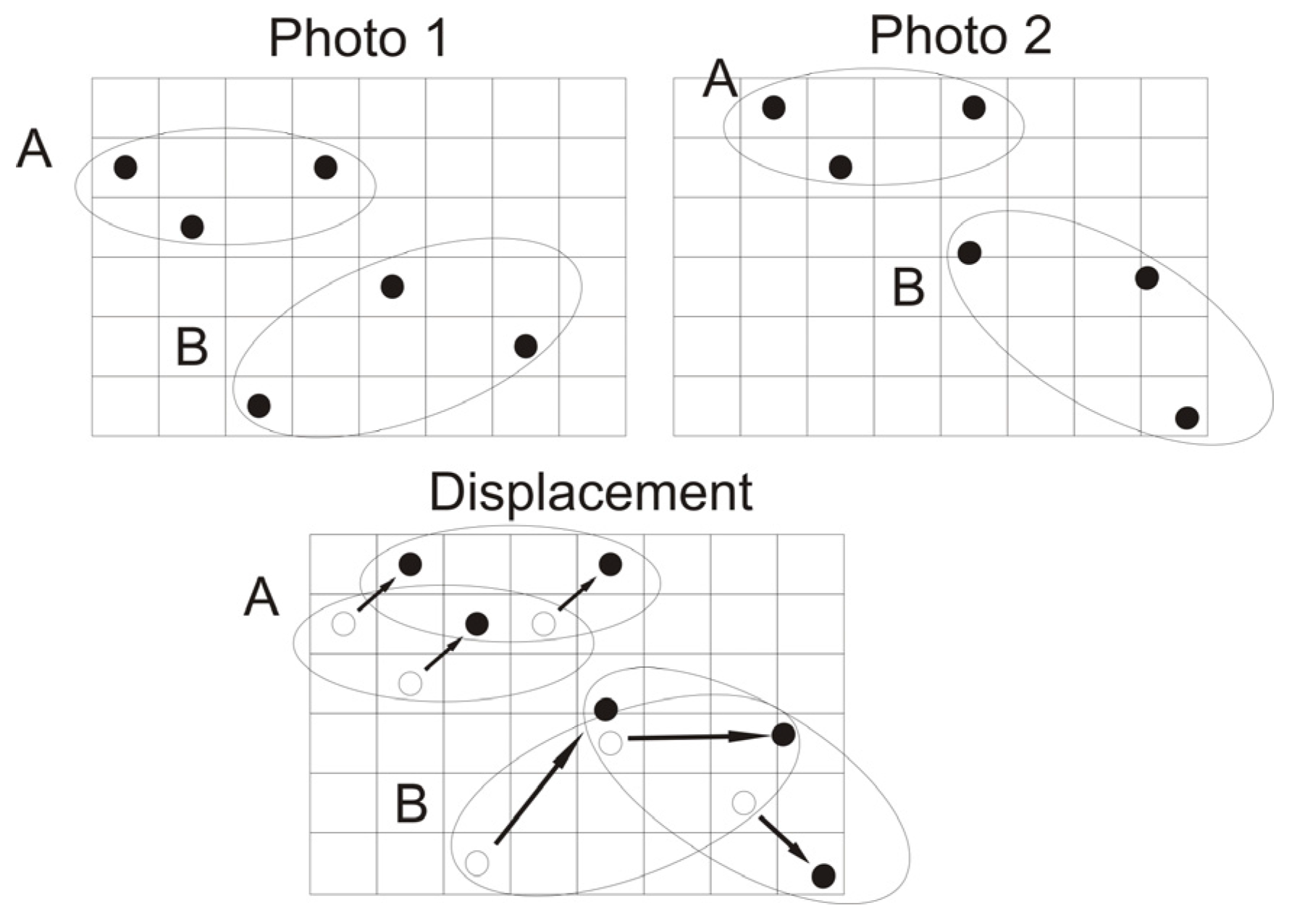
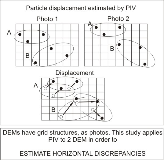
In our present study we use an approach similar to that of [8], but apply the particle image velocimetry (PIV) algorithm. PIV comes from a distant research field, more commonly used in studies involving aerodynamics [13], transonic flows [14], wind tunnels [15], or aeroacoustic predictions [16]. PIV can be used to determine the velocity field generated by a flow, tracking the particles inside that flow by repeated photography of the same area; an algorithm then computes the displacement of a particle (or a set of particles) from one photograph to the next. Dividing the particle displacement (number of pixels multiplied by the pixel size on the ground) by the time between photos gives us the velocity. Figure 3 shows how two sets of particles are displaced from Photo 1 to Photo 2.

Figure 2. Importance of vertical and horizontal accuracy.

Figure 2. Importance of vertical and horizontal accuracy.

Figure 3. Particle displacement derived from the position captured in two different photographs.

Figure 3. Particle displacement derived from the position captured in two different photographs.

A DEM resembles a digital photograph in two ways:

-

Both of them are made up of a regular grid of cells.

-

Each cell is represented by a numerical value.

For these reasons, the PIV algorithm used on photos can almost directly be applied to DEMs. The only difference is that RGB (Red, Green, Blue) color photos must be transformed to a gray scale in the case of PIV, while DEM does not require transforming the cell values.

2. Materials and Methodology

In order to test the ability of PIV in estimating the horizontal displacement between two DEMs, we adopted the dataset used in [8]. It consists of four samples (corresponding to four different places) pertaining to terrains with different slopes; they are labeled as upland, hill and mountain according to the classification from [17]. Each sample is composed of two DEMs from two different sources: “Instituto Geográfico Nacional” (IGN) [18] and “Instituto Cartográfico de Andalucía” (ICA) [19], Spanish cartographic agencies at the national and regional level, respectively. The data captured correspond to the years 2005 (IGN) and 2004 (ICA). The cell size for the ICA DEMs is 10 m, and for the IGN ones it is 25 m. This means that the IGN DEMs must be resized in order to have the same dimensions in homologous DEMs (we will refer to homologous DEMs to the sample composed for the ICA and the IGN DEMs from the same place). Once we resize an IGN DEM, its cell size is the same as the ICA one, 10 m. There are several interpolating methods that could be used for resizing the IGN DEM, taking into account the cell neighborhood, e.g., the nearest, the bilinear or the bicubic. We decided to use the bicubic one, because the interpolating method influence on the estimated horizontal displacement is small, according to the study shown in Section 3.1.

The names and the areas of each sample DEM are as follows: Seville (63.98 km²), Huétor-Tájar (34.39 km²), Colmenar (70.64 km²) and Quéntar (51.85 km²). Table 1 shows the classification and the slope value for each place.

Table 1. Slopes (%), heights (m) and category for each DEM from the dataset.

Slope (%)	Terrain category		Upland	Hill		Mountain
	Places		Seville	Huétor-Tájar	Colmenar	Quéntar
Cartographic Agencies	ICA (10 m cell size)	slope	2.66	8.24	17.93	23.28
		Height	50.29	566.4	367.30	1330.19
	IGN (25 m cell size)	slope	2.53	8.4	17.41	22.11
		Height	50.30	566.41	367.32	1330.25

Table 1. Slopes (%), heights (m) and category for each DEM from the dataset.

Slope (%)	Terrain category		Upland	Hill		Mountain
	Places		Seville	Huétor-Tájar	Colmenar	Quéntar
Cartographic Agencies	ICA (10 m cell size)	slope	2.66	8.24	17.93	23.28
		Height	50.29	566.4	367.30	1330.19
	IGN (25 m cell size)	slope	2.53	8.4	17.41	22.11
		Height	50.30	566.41	367.32	1330.25

To compare the PIV-estimated horizontal displacement (PIVEHD) with a reference displacement, we compute what we called the “real horizontal displacement” (RHD), which will be considered as the ground truth.

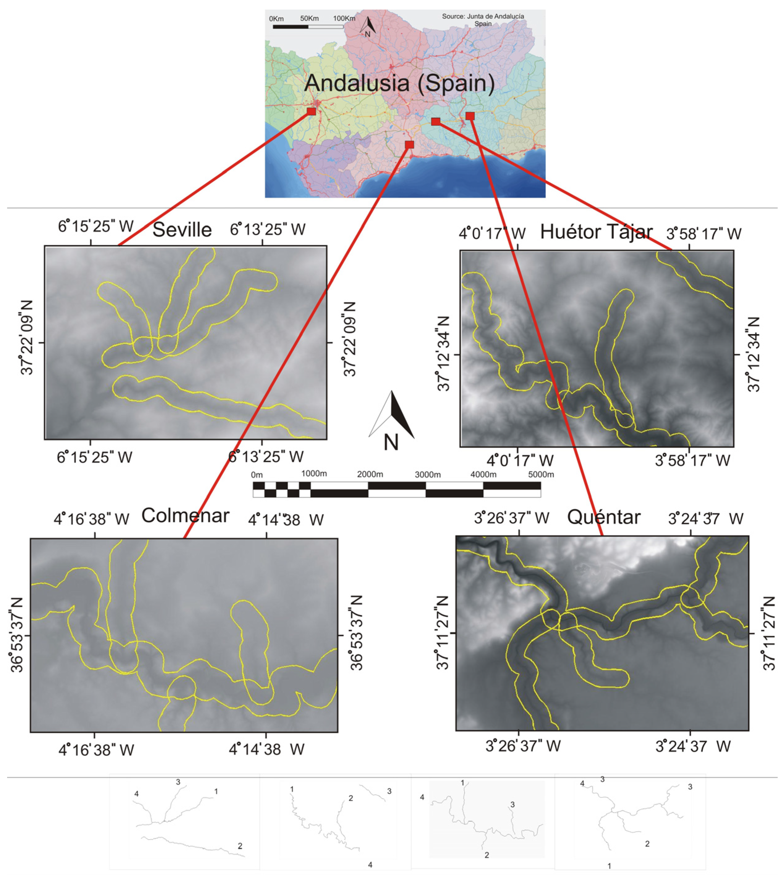
The RHD was computed by digitizing, as a polygonal shape (linear polyline), the same hydrological feature (creek or river) from the two DEM sources (ICA and IGN). Because both polygonals are in the same reference system (ETRS89 Datum) and they do not coincide exactly, the horizontal displacement can be computed as the area comprised between the two homologous polygonals and divided by their mean length. Each hydrological feature was digitized by four different people to enhance RHD accuracy. For the sake of redundancy we compute the RHD for four different hydrological features in each DEM (denoted as hydrological features 1, 2, 3 and 4 in Table 2, distributed as shown in Figure 4). Table 2 shows the RHD between homologous hydrological features and their corresponding length; the last columns give the RHD mean value for each place, taking into account the four hydrological features.

Table 2. Real displacement (RD) between homologous DEMs computed comparing linear hydrological features.

Hydrological Features	1		2		3		4
Measures	RHD (m)	Length (m)	RHD (m)	Length (m)	RHD (m)	Length (m)	RHD (m)	Length (m)	$M_{RHD}$ (m)
Quéntar	4.45	6416.92	4.75	7574.68	4.55	3530.28	4.01	2454.97	4.53
Colmenar	5.14	10,519.14	5.36	5180.19	4.99	3537.42	4.57	7054.26	5.01
Huétor-Tájar	5.03	3155.43	5.67	1356.23	5.18	2151.20	5.44	13,410.00	5.36
Seville	6.84	5279.10	6.55	3782.67	4.58	3527.30	5.01	14,224.70	5.53

Table 2. Real displacement (RD) between homologous DEMs computed comparing linear hydrological features.

Hydrological Features	1		2		3		4
Measures	RHD (m)	Length (m)	RHD (m)	Length (m)	RHD (m)	Length (m)	RHD (m)	Length (m)	$M_{RHD}$ (m)
Quéntar	4.45	6416.92	4.75	7574.68	4.55	3530.28	4.01	2454.97	4.53
Colmenar	5.14	10,519.14	5.36	5180.19	4.99	3537.42	4.57	7054.26	5.01
Huétor-Tájar	5.03	3155.43	5.67	1356.23	5.18	2151.20	5.44	13,410.00	5.36
Seville	6.84	5279.10	6.55	3782.67	4.58	3527.30	5.01	14,224.70	5.53

Figure 4. Sample DEMs (four different places) and distribution of the digitized linear hydrological features. Surrounding each hydrological feature is a buffer 600 m wide.

Figure 4. Sample DEMs (four different places) and distribution of the digitized linear hydrological features. Surrounding each hydrological feature is a buffer 600 m wide.

It may be argued that applying the PIV to the whole DEM—comparing the PIVEHD of the entire DEM with the RHD from linear hydrological features—is an over-generalization. Hence, we computed the PIVEHD inside a buffer 600 m wide surrounding each hydrological feature. This was compared to the corresponding RHD. The size and shape of the buffers can be seen in Figure 4.

Depending on the type of analysis needed, the PIV algorithm can be set with different parameters. A complete overview of PIV setting variability is found in [20]. We opted to run the algorithm based on the cross-correlation function performed under Fast Fourier Transform (FFT), taking into account that displacement could entail translation (case A in Figure 3) or a mixture of translation and rotation (case B in Figure 3), as explained in [20].

We used PIVlab software [21] to arrive at parameters suitable for the above requirements.

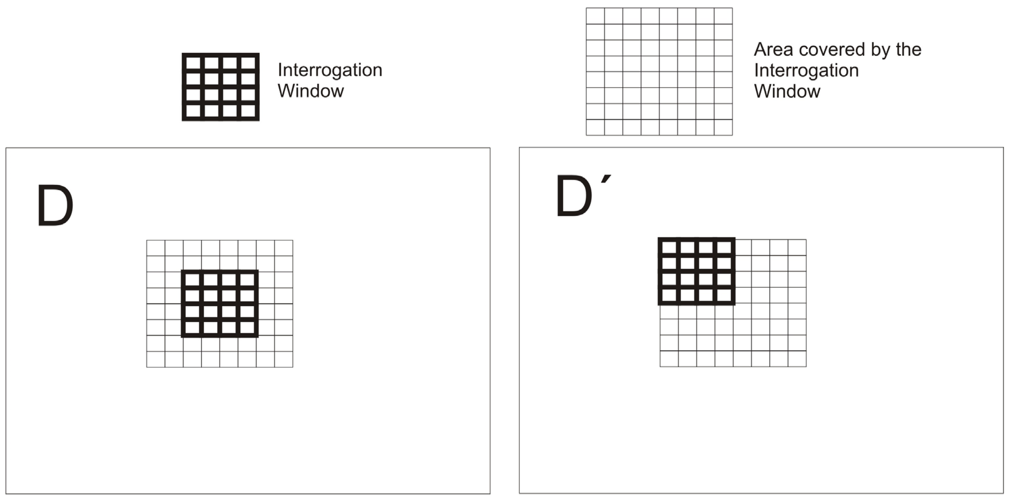
The PIV method consists of defining an interrogation window in the first DEM (D) and displacing it over the second DEM (D′) around the original position of the window in D (Figure 5).

Figure 5. Interrogation window on the first DEM (D) and a displacement over the homologous DEM (D′).

Figure 5. Interrogation window on the first DEM (D) and a displacement over the homologous DEM (D′).

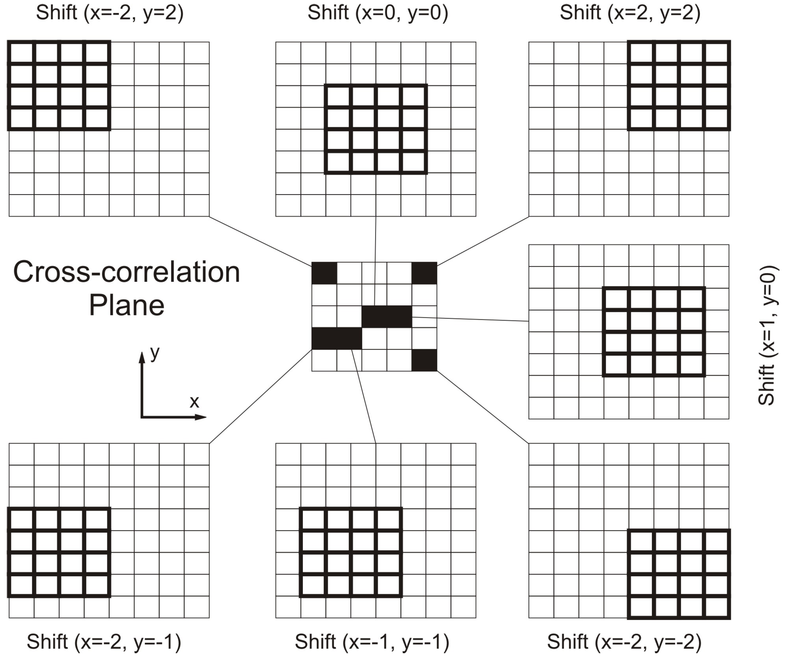
The PIV algorithm attempts to find the best match between images (in our case DEMs D and D′) using the discrete cross-correlation function defined in Equation (1).

$$R_{II}\left(x, y\right)={\displaystyle \sum }_{i=-K}^K{\displaystyle \sum }_{j=-L}^{L}H\left(i,j\right)H^{\prime }\left(i+x,j+y\right)$$

(1)

where H and H′ respectively represent the cell height in D and D′. For each displacement (x, y) selected, we obtain a $R_{II}\left(x, y\right)$ cross-correlation value. If we select a shift range $\left(-M\right)\le x\le M,-N\le y\le N$ we obtain a correlation plane of size $\left(2M+1\right)\times \left(2N+1\right)$. The cell value for the correlation plane is the sum of the products of all overlapping cells in D and D′. A graphic illustration is shown in Figure 6. The best match would be the highest cell value in the correlation plane, and therefore the displacement is the corresponding (x, y) shifts that generated such a high cell value.

Figure 6. Cross-correlation plane derived from the cross-correlation function using an interrogation window 4 × 4 in size.

Figure 6. Cross-correlation plane derived from the cross-correlation function using an interrogation window 4 × 4 in size.

The cross-correlation function as expressed in Equation 1 has two weak points:

• High computational time.
• It may produce different maximum correlation values for the same degree of matching because the function is not normalized. For example, areas with many (or brighter) particle images will produce much higher correlation values than interrogation windows with fewer (or weaker) particle images.

The solution to the first weak point is to compute the cross-correlation function as a complex conjugate multiplication of their Fourier transforms: $R_{II}=\widehat{H}·{\widehat{H\text{'}}}^{*}$, where $\widehat{H}$ and $\widehat{H\text{'}}$ are the Fourier transforms from $H$and $H^{\prime }$.

The second weak point can be overcome using the cross-correlation coefficient, which normalizes the cross-correlation function and its definition as expressed by Equation (2):

$$c_{II}\left(x,y\right)=\frac{C_{II}\left(x,y\right)}{\sqrt{{\sigma }_H\left(x,y\right)}\sqrt{{\sigma }_H^{\text{'}}\left(x,y\right)}}$$

(2)

where

$$C_{II}\left(x,y\right)={\displaystyle \sum }_{i=0}^M{\displaystyle \sum }_{j=0}^N\left[H\left(i,j\right)-{\mu }_H\right]\left[H^{\prime }\left(i+x,j+y\right)-{\mu }_{H^{\prime }\left(x,y\right)}\right]$$

(3)

$${\sigma }_H\left(x,y\right)={\displaystyle \sum }_{i=0}^M{\displaystyle \sum }_{j=0}^N{\left[H\left(i,j\right)-{\mu }_H\right]}^2$$

(4)

$${\sigma }_H^{\text{'}}\left(x,y\right)={\displaystyle \sum }_{i=0}^M{\displaystyle \sum }_{j=0}^N{\left[H^{\prime }\left(i,j\right)-{\mu }_{H^{\prime }\left(x,y\right)}\right]}^2$$

(5)

The value ${\mu }_H$ is the average of the template and is computed only once while ${\mu }_{H^{\prime }\left(x,y\right)}$ is the average of $H^{\prime }$ coincident with the template $H$at position $\left(x, y\right)$.

PIVlab [21] software offers the option of applying a multiple pass interrogation window that improves the PIV results in the sense that more particle matching is achieved in the successive passes. Each pass decreases the interrogation window size. We tried three hierarchy passes, where in the next pass the interrogation window was one half of the previous one.

3. Results and Discussion

3.1. Effect of the Interpolation Method for Resampling IGN DEM to ICA DEM on the PIVEHD

In order to study the influence of the resampling method to resize the IGN DEM to the size of the ICA DEM, we compute the differences in height for the two extreme cases, i.e., Quéntar (the steepest DEM) and Seville (the flattest DEM). If we denote a resampled DEM as $R_x^m$ where x represents the DEM (Quéntar (Q) or Seville (S)) and m represents the interpolation method (nearest (near), bilinear (bil) or bicubic (bic)), we can compute the mean difference in height for a particular DEM and two different methods, although it is most informative if we compute the mean of the absolute value of the height difference. For example considering Quéntar and the bicubic and nearest method, such a mean value will be computed as follows:

$${\mu }_Q^{bic-near}=mean\left(abs\left(R_Q^{bic}-R_Q^{near}\right)\right)$$

(6)

Table 3 shows the possible combination represented by Equation (6).

Table 3. Mean absolute differences between interpolation methods to resample the ICA DEM.

	${\mu }_x^{bic-bil}$ (m)	${\mu }_x^{bic-near}$ (m)	${\mu }_x^{bil-near}$ (m)
Quéntar	0.39	2.78	2.79
Seville	0.06	0.25	0.25

Table 3. Mean absolute differences between interpolation methods to resample the ICA DEM.

	${\mu }_x^{bic-bil}$ (m)	${\mu }_x^{bic-near}$ (m)	${\mu }_x^{bil-near}$ (m)
Quéntar	0.39	2.78	2.79
Seville	0.06	0.25	0.25

A histogram representation referring to Quéntar for the three combinations mentioned in Table 3 is shown in Figure 7.

Figure 7. Histogram from the differences between interpolation methods to resample the ICA DEM, Comparations: (a) Bicubic-Bilinear; (b) Bicubic-Nearest; (c) Bilinear-Nearest.

Figure 7. Histogram from the differences between interpolation methods to resample the ICA DEM, Comparations: (a) Bicubic-Bilinear; (b) Bicubic-Nearest; (c) Bilinear-Nearest.

From Table 3 and Figure 7 we observe than the differences between bicubic and bilinear methods are small and, when the terrain is flat like Seville, the differences between all the methods are also small. For this reason we start to compute PIV displacement for a steep area like Quéntar because if the differences between the methods are small, then in flat areas the differences will be smaller. We compute the PIVEHD using the three different IGN resampled DEMs (nearest, bilinear and bicubic) and compute the mean discrepancy in the absolute value for the module of the vector, i.e., if $U^m$ is the matrix containing the horizontal axis component for the displacement vectors, $V^m$ is the vertical axis component for the displacement vectors and m is the interpolation method (nearest, bilinear an bicubic), we can compute the effect in computing the PIVEHD using Equation (7), which considers the computation made between the bicubic and nearest interpolation methods:

$${\mu }_{diff}^{bic-near}=mean\left(sqrt\left({\left(U^{bic}-U^{near}\right)}^2+{\left(V^{bic}-V^{near}\right)}^2\right)\right)$$

(7)

The parameters used for computing PIVEHD where pass 1:32 × 32; pass 2:16 × 16; pass 3:8 × 8.

The Table 4 shows the values for the differences between methods when computing PIVEHD and the corresponding standard deviation.

Table 4. Mean differences for PIVEHD modules and standard deviations comparing pairs of interpolation methods.

	${\mu }_{diff}^{bic-bil}$ (m)	${\sigma }_{diff}^{bic-bil}$ (m)	${\mu }_{diff}^{bic-near}$ (m)	${\sigma }_{diff}^{bic-near}$ (m)	${\mu }_{diff}^{bil-near}$ (m)	${\sigma }_{diff}^{bil-near}$ (m)
Quéntar	0.04	0.11	0.16	0.17	0.16	0.18

Table 4. Mean differences for PIVEHD modules and standard deviations comparing pairs of interpolation methods.

	${\mu }_{diff}^{bic-bil}$ (m)	${\sigma }_{diff}^{bic-bil}$ (m)	${\mu }_{diff}^{bic-near}$ (m)	${\sigma }_{diff}^{bic-near}$ (m)	${\mu }_{diff}^{bil-near}$ (m)	${\sigma }_{diff}^{bil-near}$ (m)
Quéntar	0.04	0.11	0.16	0.17	0.16	0.18

From Table 4 we observe that the effect on PIVEHD is not significant either computed by the bicubic or bilinear method (4 cm), and just the near method differs with respect to bilinear and bicubic method in the same magnitude (16 cm), which is not a big value considering the cell size for ICA (10 m) and IGN (25 m). So we decide to use the bicubic interpolation method in order to resample the IGN DEM to the ICA DEM size.

3.2. Results Analysis

In order to analyze several interrogation window sizes, we tested three settings classified as High, Medium and Small. The values for such a classification are as follows:

-

High: (pass 1:64 × 64; pass 2:32 × 32; pass 3:16 × 16).

-

Medium: (pass 1:32 × 32; pass 2:16 × 16; pass 3:8 × 8).

-

Small: (pass 1:16 × 16; pass 2:8 × 8; pass 3:4 × 4).

A graphic example of applying the Medium interrogation window to the Colmenar region is shown in Figure 8. The displacement vectors are shown in green.

Table 5 shows the PIVEHD expressed in meters (Medium interrogation window setting) for each place (Quéntar, Colmenar, Huétor-Tajar and Seville), evaluated over each of their hydrological features (1, 2, 3 and 4). Although the PIVlab algorithm outputs are vectors, we compute their modules in order to know the magnitude of the displacement; the comparison shown in Table 5 refers to those modules. Remember, the horizontal displacement has been computed inside the buffer area surrounding each hydrological feature (creeks or river), as shown in Figure 4. Given in Table 5 are the respective RHDs in order to compute the error. The two last columns show the mean absolute (ABS) error for each place and the total mean ABS (error).

Figure 8. Horizontal displacement represented by vectors (green color). Detail from Colmenar DEM.

Figure 8. Horizontal displacement represented by vectors (green color). Detail from Colmenar DEM.

Table 5. PIVEHD from a Medium (pass 1:32 × 32; pass 2:16 × 16; pass 3:8 × 8) interrogation window setting and their discrepancies (ABS (error)) with respect to the RHD.

		1	2	3	4	Mean ABS (Error)	TOTAL Mean ABS (Error)
	PIVEHD	0.92	0.94	1.16	0.95		3.53
Quéntar	RHD	4.45	4.75	4.55	4.01
	Error	3.53	3.81	3.39	3.06	3.45
	PIVEHD	1.88	1.67	1.72	2.28
Colmenar	RHD	5.14	5.36	4.99	4.57
	Error	3.26	3.69	3.27	2.29	3.13
	PIVEHD	1.97	2.45	1.77	2.48
Huétor-Tajar	RHD	5.03	5.67	5.18	5.44
	Error	3.06	3.22	3.41	2.96	3.16
	PIVEHD	1.23	1.18	1.62	1.33
Seville	RHD	6.84	6.55	4.58	5.01
	Error	5.61	5.37	2.96	3.68	4.41

Table 5. PIVEHD from a Medium (pass 1:32 × 32; pass 2:16 × 16; pass 3:8 × 8) interrogation window setting and their discrepancies (ABS (error)) with respect to the RHD.

		1	2	3	4	Mean ABS (Error)	TOTAL Mean ABS (Error)
	PIVEHD	0.92	0.94	1.16	0.95		3.53
Quéntar	RHD	4.45	4.75	4.55	4.01
	Error	3.53	3.81	3.39	3.06	3.45
	PIVEHD	1.88	1.67	1.72	2.28
Colmenar	RHD	5.14	5.36	4.99	4.57
	Error	3.26	3.69	3.27	2.29	3.13
	PIVEHD	1.97	2.45	1.77	2.48
Huétor-Tajar	RHD	5.03	5.67	5.18	5.44
	Error	3.06	3.22	3.41	2.96	3.16
	PIVEHD	1.23	1.18	1.62	1.33
Seville	RHD	6.84	6.55	4.58	5.01
	Error	5.61	5.37	2.96	3.68	4.41

The mean ABS (error) shown in Table 5 seems somewhat high, particularly if compared with the estimations obtained using the optical flow algorithm [8] which had a mean error of 1.13 m. Nevertheless, the optical flow algorithm features a parameter (α) that is similar to a scale factor. For this reason, if we find a suitable scale factor that reduces the errors then PIVEHD can be considered as scalable and a good estimator of displacement. We thus propose to compute the best scale factor using the least squares method, minimizing the function$v^{T}v$ obtained from $Ax-B=v$, where A is the estimation from PIV, B is the RHD, and x is the scale factor. For example, considering Mountain terrain (Quéntar), the corresponding values are as follows: $A={\left[0.92 0.94 1.16 0.95\right]}^T$, $B={\left[4.45 4.75 4.55 4.01\right]}^T$ and $v={\left[3.53 3.81 3.39 3.06\right]}^T$

Equation (8) computes x and the standard deviation (s)

$$x={\left(A^{T}A\right)}^{-1}{A}^{T}B$$

(8)

$$s=\sqrt{\frac{v^{T}v}{dof}}$$

(9)

where dof means degrees of freedom.

The scale factors for the High, Medium and Small interrogation windows after applying the least squares methods are shown in Table 6. The values are similar, ranging from 2.937 to 2.388.

Table 6. Scale factor minimizing the PIVED errors.

Interrogation Window	High	Medium	Small
Scale Factor	2.991	2. 937	2.388
Standard Deviation	1.967	1.677	1.585

Table 6. Scale factor minimizing the PIVED errors.

Interrogation Window	High	Medium	Small
Scale Factor	2.991	2. 937	2.388
Standard Deviation	1.967	1.677	1.585

After applying the scale factor to the PIVEHD, the adjusted PIVEHD (APIVEHD) and the corresponding errors are shown (Table 7, Table 8 and Table 9), representing the High, Medium and Small interrogation windows.

Table 7. PIVED after applying the scale factor (APIVED). High interrogation window.

		1	2	3	4	Mean ABS (Error) m	TOTAL Mean ABS (Error) m	TOTAL Standard Deviation ABS (Error) m
Quéntar	APIVEHD	2.35	2.43	2.64	2.57		1.6	0.79
	ABS (error)	2.10	2.32	1.91	1.44	1.94
Colmenar	APIVEHD	5.70	5.42	4.46	6.83
	ABS (error)	−0.56	−0.06	0.53	−2.26	0.85
Huétor-Tajar	APIVEHD	4.57	7.94	4.61	6.38
	ABS (error)	0.46	−2.27	0.57	−0.94	1.06
Seville	APIVEHD	2.90	3.29	6.25	3.73
	ABS (error)	3.94	3.26	−1.67	1.28	2.54

Table 7. PIVED after applying the scale factor (APIVED). High interrogation window.

		1	2	3	4	Mean ABS (Error) m	TOTAL Mean ABS (Error) m	TOTAL Standard Deviation ABS (Error) m
Quéntar	APIVEHD	2.35	2.43	2.64	2.57		1.6	0.79
	ABS (error)	2.10	2.32	1.91	1.44	1.94
Colmenar	APIVEHD	5.70	5.42	4.46	6.83
	ABS (error)	−0.56	−0.06	0.53	−2.26	0.85
Huétor-Tajar	APIVEHD	4.57	7.94	4.61	6.38
	ABS (error)	0.46	−2.27	0.57	−0.94	1.06
Seville	APIVEHD	2.90	3.29	6.25	3.73
	ABS (error)	3.94	3.26	−1.67	1.28	2.54

Table 8. PIVED after applying the scale factor (APIVED). Medium interrogation window.

		1	2	3	4	Mean ABS (Error) m	TOTAL Mean ABS (Error) m	TOTAL Standard Deviation ABS (Error) m
Quéntar	APIVEHD	2.69	2.76	3.40	2.79		1.31	0.51
	ABS (error)	1.76	1.99	1.15	1.22	1.53
Colmenar	APIVEHD	5.51	4.91	5.04	6.71
	ABS (error)	0.37	0.45	0.05	2.14	0.75
Huétor-Tajar	APIVEHD	5.77	7.19	5.20	7.30
	ABS (error)	0.74	1.52	0.02	1.86	1.04
Seville	APIVEHD	3.60	3.47	4.76	3.90
	ABS (error)	3.24	3.08	0.18	1.11	1.9

Table 8. PIVED after applying the scale factor (APIVED). Medium interrogation window.

		1	2	3	4	Mean ABS (Error) m	TOTAL Mean ABS (Error) m	TOTAL Standard Deviation ABS (Error) m
Quéntar	APIVEHD	2.69	2.76	3.40	2.79		1.31	0.51
	ABS (error)	1.76	1.99	1.15	1.22	1.53
Colmenar	APIVEHD	5.51	4.91	5.04	6.71
	ABS (error)	0.37	0.45	0.05	2.14	0.75
Huétor-Tajar	APIVEHD	5.77	7.19	5.20	7.30
	ABS (error)	0.74	1.52	0.02	1.86	1.04
Seville	APIVEHD	3.60	3.47	4.76	3.90
	ABS (error)	3.24	3.08	0.18	1.11	1.9

Table 9. PIVED after applying the scale factor (APIVED). Small interrogation window.

		1	2	3	4	Mean ABS (Error) m	TOTAL Mean ABS (Error) m	TOTAL Standard Deviation ABS (Error) m
Quéntar	APIVEHD	3.03	3.06	3.46	2.96		1.42	0.36
	ABS(error)	1.42	1.69	1.09	1.05	1.31
Colmenar	APIVEHD	4.20	3.75	4.06	5.08
	ABS(error)	0.94	1.61	0.93	0.51	1.00
Huétor-Tajar	APIVEHD	6.85	7.44	6.60	7.84
	ABS(error)	1.82	1,77	1,42	2.40	1.85
Seville	APIVEHD	4.61	4,25	4,10	3.92
	ABS(error)	2.23	2.30	0.48	1.09	1.53

Table 9. PIVED after applying the scale factor (APIVED). Small interrogation window.

		1	2	3	4	Mean ABS (Error) m	TOTAL Mean ABS (Error) m	TOTAL Standard Deviation ABS (Error) m
Quéntar	APIVEHD	3.03	3.06	3.46	2.96		1.42	0.36
	ABS(error)	1.42	1.69	1.09	1.05	1.31
Colmenar	APIVEHD	4.20	3.75	4.06	5.08
	ABS(error)	0.94	1.61	0.93	0.51	1.00
Huétor-Tajar	APIVEHD	6.85	7.44	6.60	7.84
	ABS(error)	1.82	1,77	1,42	2.40	1.85
Seville	APIVEHD	4.61	4,25	4,10	3.92
	ABS(error)	2.23	2.30	0.48	1.09	1.53

Comparing Table 5 and Table 8, both corresponding to the Medium interrogation window, we note an improvement (Impv) of 2.22 m through application of the scale factor. This amounts to a substantial improvement (62.9%):

$$Impv=errorWithoutScaFactor-errorAfterScaFactor=3.53-1.31=2.22$$

(10)

Given that the cell size of the ICA DEMs is 10 m, and the best error corresponds to the Medium interrogation window (1.31 m), we may conclude that the PIV algorithm is a sound estimator of horizontal displacement between homologous DEMs: the error is around one-seventh of the corresponding cell size. On the other hand, if we consider the IGN cell size, the proportion decreases to one-nineteenth.

In general, no great differences are observed among the errors of the three categories (High, Medium and Small); the dispersion appears to decrease when the interrogation window decreases (see the values for the Total Standard Deviation ABS (error) in Table 7, Table 8 and Table 9). However, if we were to recommend an interrogation window, it would be the Small one, in view of its reduced Total Standard Deviation ABS (error) value. Notwithstanding, the Medium category offers the advantage of a shorter processing time.

3.2.1. Performance in Comparison to Previous Approaches

As mentioned in the abstract and the Introduction section, there are barely any algorithms analyzing horizontal displacement on homologous DEMs as a whole. Just the contour-based [7] and optical flow [8] approaches study the DEM horizontal variable. So we consider it necessary to compare the performance between both algorithms, and such a performance is studied considering the absolute error between the ground truth and the estimation achieved by every approach (contour, optical flow and PIV). An additional comparison concerning computation time has been added in order to assess the global performance. Absolute error and computation time are shown in Table 10. The computer used to test the mentioned algorithms had the following features: Intel i5 processor, 8 Gb RAM, 256 SSD hard drive, Windows 7 operating system.

Table 10. Horizontal displacement absolute errors and computation time obtained using contours, optical flow and PIV approaches.

		Quéntar	Colmenar	Huétor-Tájar	Seville
Contour-based	ABS (error)	0.52	0.44	0.48	0.52
	Computation Time (seconds)	548	639	568	677
Optical Flow	ABS (error)	0.39	0.42	0.56	3.18
	Computation Time (seconds)	122	165	130	151
APIVEHD	ABS (error)	1.53	0.75	1.04	1.9
	Computation Time (seconds)	143	173	155	184

Table 10. Horizontal displacement absolute errors and computation time obtained using contours, optical flow and PIV approaches.

		Quéntar	Colmenar	Huétor-Tájar	Seville
Contour-based	ABS (error)	0.52	0.44	0.48	0.52
	Computation Time (seconds)	548	639	568	677
Optical Flow	ABS (error)	0.39	0.42	0.56	3.18
	Computation Time (seconds)	122	165	130	151
APIVEHD	ABS (error)	1.53	0.75	1.04	1.9
	Computation Time (seconds)	143	173	155	184

From Table 10, Mountain and Hill terrains have been similarly estimated by contour and optical flow algorithms, and both get better estimations than the APIVEHD one. On the computation time side, optical flow had the best performance; it is even better than APIVEHD although the differences are not very large (around 14% better than APIVEHD). Although the best horizontal displacement comes from the contour-based algorithm, its computation time is 4.28× larger than optical flow and 3.71× larger than APIVEHD.

Likewise, the error values obtained for Seville, a nearly flat region (2.6% slope), are noteworthy. On such a terrain type, the horizontal displacement errors increase quickly [8]. In our case, the APIVEHD algorithm improves results for nearly flat terrains with respect to the optical flow approach, namely 1.9 m for the APIVEHD algorithm versus 3.18 m for the optical flow algorithm, although the contour algorithm keeps the best performance. We can see from Table 10 that the steeper the terrain the better the optical flow algorithm performs; nevertheless, in near-flat areas the APIVEHD approach achieves the best estimation. Taking into account both absolute error and computation time, we think that our new proposed algorithm APIVEHD gets a better tradeoff when we estimate the horizontal displacement in near-flat areas such as Seville.

3.2.2. Assessing the Influence of DEM Cell Size on the APIVEHD Algorithm Results

After computing the scale factor, the results obtained from the APIVEHD applied to our dataset seem to be suitable for estimating the horizontal displacement (Table 7, Table 8 and Table 9), but there is a variable that could be modified for suitable estimation yield by APIVEHD; this variable is the cell size ratio between the DEMs compared. Our study, resumed in Table 7, Table 8 and Table 9, compared IGN (25 m cell size) and ICA (10 m cell size). In order to evaluate the ability of APIVEHD to get a suitable estimation of horizontal displacement across different cell size ratios, we modified the cell size for ICA to 15 m and 25 m and then we applied the APIVEHD algorithm again, comparing those cell sizes (15 m and 25 m) against the IGN DEM (25 m). According to Section 3.1, the bicubic and bilinear resampling methods are similar and practically do not influence the results yielded by APIVEHD; for this reason, we select the bicubic method in order to compute the derived ICA 15 m and 25 m cell sizes in order to assess the effect of using different cell size ratios between DEMs when computing the horizontal displacement with APIVEHD.

For the sake of readability we just present in Table 11 the horizontal displacement between the following homologous DEMs whose cell sizes are inserted in their names: (1) IGN25m-ICA15m; (2) IGN25m-ICA25m. Note that IGN25m-ICA10m corresponds to Table 8. We selected Table 8 as the reference because the Medium interrogation window has the smaller mean absolute error.

Table 11. APIVEHD obtained by comparison between the homologous pairs DEMs IGN25m-ICA15m and between the homologous IGN25m-ICA25m.

			1	2	3	4	Mean ABS (Error) m	TOTAL Mean ABS (Error) m	TOTAL Standard Deviation ABS (Error) m
IGN25m-ICA15m	Quéntar	APIVEHD	2.81	3.63	3.58	2.55		1.47	0.16
		ABS (error)	1.64	1.12	0.97	1.46	1.3
	Colmenar	APIVEHD	4.63	3.02	3.25	5.78
		ABS (error)	0.51	2.34	1.74	1.21	1.45
	Huétor-Tajar	APIVEHD	3.77	7.25	6.77	6.78
		ABS (error)	1.26	1.58	1.59	1.34	1.44
	Seville	APIVEHD	4.93	4.78	3.23	3.31
		ABS (error)	1.91	1.77	1.35	1.7	1.68
IGN25m-ICA25m	Quéntar	APIVEHD	3.21	3.17	3.22	2.64		1.57	0.22
		ABS (error)	1.24	1.58	1.33	1.37	1.38
	Colmenar	APIVEHD	3.53	3.29	2.73	5.95
		ABS (error)	1.61	2.07	2.26	1.38	1.83
	Huétor-Tajar	APIVEHD	3.26	7.08	6.98	3.66
		ABS (error)	1.77	1.41	1.8	1.78	1.69
	Seville	APIVEHD	7.21	4.58	2.86	3.51
		ABS (error)	0.37	1.97	1.72	1.5	1.39

Table 11. APIVEHD obtained by comparison between the homologous pairs DEMs IGN25m-ICA15m and between the homologous IGN25m-ICA25m.

			1	2	3	4	Mean ABS (Error) m	TOTAL Mean ABS (Error) m	TOTAL Standard Deviation ABS (Error) m
IGN25m-ICA15m	Quéntar	APIVEHD	2.81	3.63	3.58	2.55		1.47	0.16
		ABS (error)	1.64	1.12	0.97	1.46	1.3
	Colmenar	APIVEHD	4.63	3.02	3.25	5.78
		ABS (error)	0.51	2.34	1.74	1.21	1.45
	Huétor-Tajar	APIVEHD	3.77	7.25	6.77	6.78
		ABS (error)	1.26	1.58	1.59	1.34	1.44
	Seville	APIVEHD	4.93	4.78	3.23	3.31
		ABS (error)	1.91	1.77	1.35	1.7	1.68
IGN25m-ICA25m	Quéntar	APIVEHD	3.21	3.17	3.22	2.64		1.57	0.22
		ABS (error)	1.24	1.58	1.33	1.37	1.38
	Colmenar	APIVEHD	3.53	3.29	2.73	5.95
		ABS (error)	1.61	2.07	2.26	1.38	1.83
	Huétor-Tajar	APIVEHD	3.26	7.08	6.98	3.66
		ABS (error)	1.77	1.41	1.8	1.78	1.69
	Seville	APIVEHD	7.21	4.58	2.86	3.51
		ABS (error)	0.37	1.97	1.72	1.5	1.39

From the comparison of Table 8 and Table 11, we do not observe large variations in the TOTAL mean ABS (error). The error estimating the horizontal displacement when we increase the ICA cell size by 5 m is 1.47, just 0.16 m if compared with original ICA cell size, i.e., the influence of the cell size ratio (IGN25m-ICA10m versus IGN25m-ICA10m) in the horizontal displacement estimation by APIVEHD is just 16 cm. The influence in the case of IGN25m-ICA10m versus IGN25m-ICA25m is 0.26 m. Both effects, 0.16 m and 0.26 m, seem to indicate that the APIVEHD algorithm remains robust to the variation in the cell size ratio.

4. Conclusions

In our study we compute the horizontal displacement between two homologous DEMs coming from different sources. This is important because the horizontal discrepancy in both DEMs puts some derived features in non-corresponding places (e.g., hydrological linear features). Such discrepancies may be estimated by using the PIV algorithm as proposed in this paper. However, a larger number of cases must be computed in order to completely generalize our results. Our findings are a novelty in that an algorithm from the distant disciplines of aerodynamics or water flows is here applied to the DTM field.

The PIV algorithm underestimates the real horizontal displacement, but it does so in a scalar sense, which means that it as a scale factor can be used to arrive at a suitable estimation.

Using PIV and applying the scale factor, the error is around one-seventh of the cell size of the smaller DEMs (the ICA DEMs) and around one-nineteenth in the case of the larger cell size DEMs (the IGN DEMs). We consider these to be acceptable error values.

One remarkable finding is that the PIV approach provides reliable horizontal displacement values for nearly flat terrain types, which are the most difficult ones to compute due to their horizontal displacement.

The recommended interrogation windows are similar to those recommended in the original fields of PIV (aerodynamics, fluid mechanics...), i.e., 32 × 32 [20].

Future works along these lines will involve exploring PIV behavior in the horizontal displacement estimation between DEMs derived from LiDAR (very small cell sizes) and photogrammetry (cell sizes similar to the one used here). It would be interesting to determine whether the three interrogation window categories produce results that agree with the results presented here, or if new dimensions for the interrogation windows are necessary. In the case of LiDAR, because the cell size could be around a few centimeters, it would likely be better to use smaller features than hydrological ones, in order to compute the ground truth for the horizontal displacement, e.g., houses, buildings, fences, small dams, small pieces of roads. Another important point will be the computation time, because if we want to analyze a significant area, the file size will increase considerably, as will the PIV computation. Such a situation could need to parallelize some functions from the PIV software.

References

1. Gao, J. Resolution and accuracy of terrain representation by grid DEMs at a micro-scale. Int. J. Geogr. Inf. Sci. 1997, 11, 199–212. [Google Scholar] [CrossRef]
2. Torlegard, K.; Ostman, A.; Lindgren, R. A comparative test of photogrammetrically sampled digital elevation models. Photogrammetria 1986, 41, 1–16. [Google Scholar] [CrossRef]
3. Aryal, S.K.; Bates, B.C. Effects of catchment discretization on topographic index distributions. J. Hydrol. 2008, 359, 150–163. [Google Scholar] [CrossRef]
4. Wise, S. Effect of differing DEM creation methods on the results from a hydrological model. Comput. Geosci. 2007, 33, 1351–1365. [Google Scholar] [CrossRef]
5. McAlister, E.; Domburg, N.; Edwards, T.; Ferrier, B. Hydrological modelling of the river Ythan using Arcinfo Grid. In Proceedings of Sixteenth Annual ESRI User Conference, California, CA, USA, 20–24 May 1996; pp. 253–261.
6. Reinoso, J.F. A priori horizontal displacement (HD) estimation of hydrological features when versioned DEMs are used. J. Hydrol. 2010, 384, 130–141. [Google Scholar] [CrossRef]
7. Reinoso, J.F. An algorithm for automatically computing the horizontal shift between homologous contours from DTMs. ISPRS J. Photogramm. Remote Sens. 2011, 66, 272–286. [Google Scholar] [CrossRef]
8. Reinoso, J.F.; León, C.; Mataix, J. Optical flow algorithm as estimator of horizontal discrepancy between features derived from DEMs: Rivers and creeks as case study. Surv. Rev. 2014, 46, 149–154. [Google Scholar] [CrossRef]
9. TERC (Tahoe Environmental Research Center). Available online: http://terc.ucdavis.edu/research/storm-water/detention-basin.html (accessed on 24 November 2015).
10. Bencardino, M. Preparation and processing of optical images (photographs and satellite) for the determination of landslide displacement field. In Proceedings of the Seventh International Conference on Informatics and Urban and Regional Planning INPUT 2012, Cagliary, Italy, 10–12 May 2012; pp. 1202–1214.
11. Delacourt, C.; Allemand, P.; Casson, B.; Vadon, H. Velocity fields of the “La Clapiere” landslide measured by the correlation of aerial and QuickBirdsatellite images. Geophys. Res. Lett. 2004. [Google Scholar] [CrossRef]
12. Vadon, H.; Massonnet, D. Earthquake displacement fields mapped by very precise correlation: Complementarity with radar interferometry. In Proceedings of the IEEE 2002 International Geoscience and Remote Sensing Symposium, Toronto, ON, Canada, 24–28 June 2002.
13. Richard, H.; van der Wall, B.G. Detailed investigation of rotor blade tip vortex in hover condition by 2C and 3C-PIV. In Proceedings of the 32nd European Rotorcraft Forum, Maastricht, The Netherlands, 12–14 September 2006.
14. Scarano, F.; van Oudheusden, B.W. Planar velocity measurements of a two-dimensional compressible wake flow. Exp. Fluids 2003, 34, 430–441. [Google Scholar] [CrossRef]
15. Berton, E.; Favier, D.; NsiMba, M.; Maresca, C.; Allain, C. Embedded LDV measurements methods applied to unsteady flow investigation. Exp. Fluids 2001, 30, 102–110. [Google Scholar] [CrossRef]
16. Schram, C.; Hirschberg, A. Application of vortex sound theory to vortex-pairing noise: Sensitivity to errors in flow data. J. Sound Vib. 2003, 266, 1079–1098. [Google Scholar] [CrossRef]
17. Li, Z.; Zhu, Q.; Gold, C. Digital TerrainModeling; CRC Press: Boca Raton, FL, USA, 2005. [Google Scholar]
18. IGN (Instituto Geográfico Nacional de España), 2006. Modelo Digital del Terreno Escala 1:25,000. Ministerio de Fomento. Available online: http://centrodedescargas.cnig.es/CentroDescargas/index.jsp (accessed on 15 July 2014).
19. De Andalucía, J. Modelo digital del terreno de andalucía. relieve y orografía. ICA [DVD] 2005, 1, 10–27. [Google Scholar]
20. Raffel, M.; Willert, C.; Wereley, S.; Kompenhans, J. Particle Image Velocimetry. A Practical Guide; Springer: Berlin, Germany, 2007. [Google Scholar]
21. Thielicke, W.; Stamhuis, E.J. PIVlab-Time-Resolved Digital Particle Image Velocimetry Tool for MATLAB (Version: 1.32). Available online: http://dx.doi.org/10.6084/m9.figshare.1092508 (accessed on 15 April 2014).