Application of Synthetic NDVI Time Series Blended from Landsat and MODIS Data for Grassland Biomass Estimation

Abstract

Accurate monitoring of grassland biomass at high spatial and temporal resolutions is important for the effective utilization of grasslands in ecological and agricultural applications. However, current remote sensing data cannot simultaneously provide accurate monitoring of vegetation changes with fine temporal and spatial resolutions. We used a data-fusion approach, namely the spatial and temporal adaptive reflectance fusion model (STARFM), to generate synthetic normalized difference vegetation index (NDVI) data from Moderate-Resolution Imaging Spectroradiometer (MODIS) and Landsat data sets. This provided observations at fine temporal (8-d) and medium spatial (30 m) resolutions. Based on field-sampled aboveground biomass (AGB), synthetic NDVI and support vector machine (SVM) techniques were integrated to develop an AGB estimation model (SVM-AGB) for Xilinhot in Inner Mongolia, China. Compared with model generated from MODIS-NDVI (R² = 0.73, root-mean-square error (RMSE) = 30.61 g/m²), the SVM-AGB model we developed can not only ensure the accuracy of estimation (R² = 0.77, RMSE = 17.22 g/m²), but also produce higher spatial (30 m) and temporal resolution (8-d) biomass maps. We then generated the time-series biomass to detect biomass anomalies for grassland regions. We found that the synthetic NDVI-derived estimations contained more details on the distribution and severity of vegetation anomalies compared with MODIS NDVI-derived AGB estimations. This is the first time that we have generated time series of grassland biomass with 30-m and 8-d intervals data through combined use of a data-fusion method and the SVM-AGB model. Our study will be useful for near real-time and accurate (improved resolutions) monitoring of grassland conditions, and the data have implications for arid and semi-arid grasslands management.

1. Introduction

Grasslands are of considerable global importance because they are important sites for biodiversity and serve as energy suppliers for mankind (i.e., production of agricultural commodities such as hay and livestock); grassland conservation is a particular concern in China because of land use changes due to climate variability and the country’s continued population growth [1]. Dynamic pasture growth information is of great significance for pasture capacity enhancements, the development of appropriate management strategies and rotational grazing plans, regional livestock production, and scientific evaluations of ecological benefits. In grassland ecosystems, the amount of biomass represents primary production and determines the herbivore carrying capacity [2]. It can also reflect the health status of grassland ecosystems. Therefore, accurate estimates of grassland biomass are critical for their management.

Field surveys are the most reliable method to obtain accurate grassland biomass data, but these surveys are extremely time-consuming and labor-intensive over large areas, especially in remote regions. Satellite platforms offer an effective way to collect data over large areas [3]. The normalized difference vegetation index (NDVI) is the most widely known vegetation index that can be computed from remotely sensed data (e.g., Landsat and Moderate-Resolution Imaging Spectroradiometer (MODIS) data), and the NDVI has been shown to be a sufficiently stable indicator for monitoring the intra- and inter-annual variations of vegetation greenness [4]. However, technical and financial constraints often limit the remote sensing instruments’ ability to acquire data with high spatial and temporal resolutions simultaneously [5]. For example, remotely sensed images acquired from Landsat satellites have a spatial resolution of 30 m for multispectral bands. However, its long revisit cycle of 16 d, frequent cloud contamination, and other poor atmospheric conditions that are often encountered [6,7,8] limit the uses of Landsat data. In contrast, MODIS data can provide highly frequent (daily) observations. However, their coarse spatial resolutions ranging from 250 to 1000 m restrict their applications in relatively small and heterogeneous landscapes. Thus, integrating information from different remote sensing sensors with image fusion techniques could be a feasible and inexpensive way to better capture land surface characteristics [9].

Traditional image fusion methods such as intensity-hue-saturation (IHS) transformation [10], principal component analysis [11], and wavelet decomposition [12] are not effective for generating synthetic observations with enhanced spatiotemporal resolution [12,13]. While these traditional methods can be used to combine high spatial resolution panchromatic images and spectral information for coarse pixel images, they cannot generate time series of reflectance with both high spatial and temporal information [14]. Thus, the panchromatic images can only help to enhance the spatial resolution [15]. In order to generate reflectance data with both high spatial and temporal resolution, Gao et al. [14] developed a Spatial and Temporal Adaptive Reflectance Fusion Model (STARFM) for the prediction of daily surface reflectance through blending Landsat and MODIS data. The STARFM algorithm has been applied successfully in several studies involved with the monitoring of seasonal changes in surface features [16,17,18,19], improving the accuracy of classifications [20], and evaluating gross primary productivity (GPP) [21]. Through adopting the synthetic reflectance series generated by STARFM, Singh [22] found that the GPP derived from synthetic reflectance data could effectively capture the green-up and leaf down dates of croplands over the growing season. Bhandari et al. [23] fused MODIS and Landsat data through the use of STARFM and generated synthetic surface reflectance data to replace low-quality Landsat thematic mapper (TM) images contaminated by clouds. Consequently, they acquired a long 5-yr time series at Landsat resolution. They found that this Landsat image series, which had resolutions of 16 d and 30 m, could be effectively used to monitor vegetation phenology in broadleaf forest environments. Senf et al. [24] performed land cover classifications by detecting the phenology patterns of different vegetation with the synthetic NDVI series and found that synthetic images could be used to compensate for missing Landsat data and increase the classification accuracy compared to that with the use of single-date Landsat data. Based on the design of STARFM, several new methods and modifications have been developed, including the sparse-representational-based spatiotemporal reflectance fusion model (SPSTFM) [25], enhanced spatial and temporal adaptive reflectance fusion model (ESTARFM) [15], spatial temporal adaptive algorithm for mapping reflectance change (STAARCH) [26], spatial and temporal reflectance unmixing model (STRUM) [27], and other fusion algorithms [13,28,29,30]. Most of these methods need more than one image pair as inputs. However, it is very hard to acquire many scenes of TM data without cloud contamination. The STARFM is the most widely used method and can work with a single pair of fine and coarse images. Moreover, the STARFM has achieved satisfactory results in many studies [18,22,23,31,32], which have demonstrated its practicability.

Various methods have been applied with remotely sensed data for estimating grassland biomass, and these methods include multiple regression analysis [33], K-nearest neighbor [34], artificial neural network (ANN) [35], and support vector machine (SVM) techniques. Artificial neural network, because of its ability to handle complex nonlinear functions, has been successfully used in various land observation applications including biomass estimations [35,36,37], land classifications [38,39], and land change detection [40,41]. However, the ANN model would not produce guaranteed accuracy when there are not enough samples and it is easy to over-fit the data when there are excessive numbers of samples [42]. Support vector machine is based on the structural risk minimization principle and isgood at solving practical problems involving small numbers of training samples, nonlinearity, high numbers of dimensions, and local minima; thus, SVM is considered to be a good alternative to ANN. Several studies have demonstrated that biomass estimation based on a SVM model can provide robust results [43,44,45].

The objective of this study was to accurately estimate aboveground biomass (AGB) for grasslands in arid and semi-arid regions of Inner Mongolia, China. To achieve this goal, we first derived synthetic NDVI time series with high temporal and spatial resolution by blending the high-temporal MODIS data and the medium-spatial Landsat data with a data-fusion approach. We then developed different biomass models and integrated the synthetic NDVI products to acquire the optimal grassland AGB estimation model for accurate estimates of AGB (8-d intervals and 30-m resolutions). To further explore the practicability of our model, we calculated biomass anomalies with the optimal grassland AGB estimation model and further compared the results between the synthetic NDVI-derived biomass and the MODIS NDVI-derived biomass data. Our approach detailed in this study will be useful for near real-time and accurate (high spatial and temporal resolutions) monitoring of grasslands conditions. Such data have the potential to help grassland managers utilize grassland resources more effectively.

2. Study Area and Data

2.1. Study Area

Xilinhot (Figure 1) is located in the hinterland of Xilingol, and covers an area of about 15,000 km² (43°02′–44°52′N, 115°13′–117°06′E). The elevation in this area shows a decreasing gradient from the southeast to the northwest. This area is characterized by a typical temperate continental semi-arid climate. Winters are cold and dry, where conditions are influenced by the air flow from the Mongolian plateau, whereas summers are wet and warm, where conditions are influenced by monsoons. This area has an average annual temperature of 0.5–1.0 °C and an annual mean precipitation of 350 mm. Precipitation is often distributed unevenly in the region, and droughts occur frequently [46]. In addition, 90% of this area is dominated by temperate steppe, and the typical growing season is from May to September. Grassland biomass shows a decreasing trend from southeast to northwest that follows the elevation transition in the study area [35,47].

Figure 1. The location of Xilinhot. The elevation in the left-bottom corner was generated by using Shuttle Radar Topography Mission (SRTM) data (http://srtm.csi.cgiar.org/). The image on the right is the RGB (red, green, blue) composite of Landsat bands 5, 4, and 3 overlaid with field locations (orange dots) where samples were collected in 2011.

Figure 1. The location of Xilinhot. The elevation in the left-bottom corner was generated by using Shuttle Radar Topography Mission (SRTM) data (http://srtm.csi.cgiar.org/). The image on the right is the RGB (red, green, blue) composite of Landsat bands 5, 4, and 3 overlaid with field locations (orange dots) where samples were collected in 2011.

2.2. Field Data

We sampled 68 samples during the growing season of 2011 (10 June to 15 June and 20 July to 25 July), and sample locations are indicated with the orange dots in Figure 1. Distances between samples were at least 1.5 km to avoid spatial auto-correlation. The size of each sample was 300 m × 300 m to provide overlapping coverage for the corresponding MODIS pixel (250 m × 250 m). Given the high cost associated with sampling biomass in such large sample areas, and the fact that endemic grass species are not very heterogeneous within the 300 m × 300 m plots, we subsampled the large sample areas by using five 1 m × 1 m quadrats (one in the center and four about 100–150 m away from the center); the data from the subsamples were then used to represent the grassland growth conditions of the corresponding sample area. Specifically, plants in each 1 m × 1 m quadrant were clipped to the ground surface and then dried at 70 °C to obtain the dry weight. The average dry weight of the five 1 m × 1 m quadrats was calculated and used to represent the mean biomass of the 300 m × 300 m sample [48].

2.3. Remote Sensing Data

Landsat TM and MODIS data were used to generate the primary inputs for the STARFM fusion model. We obtained 12 scenes of Landsat 5 TM images (path 124/row 29, path 124/row 30, cloud cover <10%) covering the years of 2005–2011 (Table 1), and the data were processed with Landsat Ecosystem Disturbance Adaptive Processing System (LEDAPS) tools. The LEDAPS software was developed specifically for processing Landsat directional surface reflectance data through radiometric calibration, atmospheric correction, image registration, and image orthorectification [49]. The digital numbers (DNs) of the Landsat TM images were converted to reflectance values based on the atmospheric calibration procedure that was implemented by using LEDAPS [50].

The MODIS product (MOD09Q1, tile h26v04) at 250 m and 8-d intervals for the study area during the growing season (May to September) in 2005–2013 was obtained from the National Aeronautics and Space Administration’s (NASA’s) Earth Observing System Data and Information System (http://earthdata.nasa.gov). The MOD09Q1 product contains optimal observations during the 8-d periods given the effects of clouds, cloud shadows, and aerosol loading [51]; pixels with poor quality were excluded by using the quality assurance layer. The MODIS reflectance imagery were projected to Universal Transverse Mercator (UTM) projections and resampled to a 30-m resolution by nearest neighbor resampling to meet the projection and resolution of Landsat TM data.

Table 1. Landsat and Moderate Resolution Imaging Spectroradiometer (MODIS) image pairs for generating synthetic Normalized Difference Vegetation Index (NDVI) data during 2005–2013. Years highlighted with bold font lacked Landsat images, and therefore, the Landsat images from adjacent year (1-yr interval) or 2-yr intervals were used.

Year	Landsat TM Path = 124, Row = 29/30	MODIS (DOY) Tile = h26v04
2005	09/02/2005	241/2005
2006	09/21/2006	265/2006
2007	09/08/2007	249/2007
2008	09/08/2007	249/2007
2009	08/12/2009	225/2009
2010	08/31/2010	241/2010
2011	08/02/2011	209/2011
2012	08/02/2011	209/2011
2013	08/02/2011	209/2011

Table 1. Landsat and Moderate Resolution Imaging Spectroradiometer (MODIS) image pairs for generating synthetic Normalized Difference Vegetation Index (NDVI) data during 2005–2013. Years highlighted with bold font lacked Landsat images, and therefore, the Landsat images from adjacent year (1-yr interval) or 2-yr intervals were used.

Year	Landsat TM Path = 124, Row = 29/30	MODIS (DOY) Tile = h26v04
2005	09/02/2005	241/2005
2006	09/21/2006	265/2006
2007	09/08/2007	249/2007
2008	09/08/2007	249/2007
2009	08/12/2009	225/2009
2010	08/31/2010	241/2010
2011	08/02/2011	209/2011
2012	08/02/2011	209/2011
2013	08/02/2011	209/2011

3. Methods

3.1. Procedure for Grassland AGB Estimation

The development of the AGB estimation model took place via four main steps (Figure 2).

Step I: Generation of synthetic NDVI by using STARFM. We obtained the synthetic NDVI for the AGB estimation model based on STARFM with the Landsat spatial resolution and MODIS temporal frequency. The base data pairs are shown in Table 1. The STARFM algorithm is described in more details in Section 3.2.

Step II: Development of the AGB estimation model. A total of 68 field samples were collected during June to August in 2011, and these data were used for the development and validation of the AGB model. We used the training set (46 samples) to construct four AGB estimation models, including linear regression model, power function model, exponential model, and SVM model. We then used the remaining of 22 plots (1/3 of the samples) as the testing data set to evaluate the four AGB estimation models.

Figure 2. Procedures for developing the aboveground biomass (AGB) estimation model. Pre_NDVI represents the synthetic NDVI series.

Figure 2. Procedures for developing the aboveground biomass (AGB) estimation model. Pre_NDVI represents the synthetic NDVI series.

Step III: Choose the optimal model for biomass estimation. To evaluate the model’s performance, we used three statistical indices, namely, the coefficient of determination (R²), root-mean-square error (RMSE), and relative RMSE (RMSE_r) [52]. The RMSE and RMSE_r were calculated as follows:

$$RMSE = \sqrt{{\displaystyle \sum }_{i = 1}^n{\left(y_i-\widehat{y_i}\right)}^2/n}$$

(1)

$$RMS{E}_r = \left(\sqrt{{\displaystyle \sum }_{i = 1}^n{\left(y_i-\widehat{y_i}\right)}^2/n}/\overline{\widehat{y_i}}\right)\times 100\%$$

(2)

where ${\text{y}}_{\text{i}}$ is the observed value, $\widehat{{\text{y}}_{\text{i}}}$ is the model predicted value, $\overline{\widehat{{\text{y}}_{\text{i}}}}$ is the mean of the modeled values, and n is the sample number. In this study, we found that the SVM (see Section 3.3) was the optimal model for biomass estimation in this region.

Step IV: The Standardized Anomalies Index (SAI) [53] was used to detect the spatial and temporal distribution of biomass anomalies in July 2007. The SAI is defined as follows:

$$SA{I}_{AGB}= (AG{B}_i-\overline{AGB})/{\sigma }_{AGB}$$

(3)

Here, $SA{I}_{AGB}$represents the AGB anomalies, $AG{B}_i$ is the annual AGB in the $ith$ year, $\overline{AGB}$ is the mean AGB for the years of 2005–2013, and ${\sigma }_{AGB}$ is the standard deviation of the 9-yr AGB. Positive SAI values indicate that the annual AGB is larger than the 9-yr mean, while negative SAI values indicate that the annual AGB is more deficient compared to the 9-yr mean. In this study, we compared the $SA{I}_{AGB}$generated from the synthetic NDVI-derived biomass images and from the MODIS NDVI-derived biomass images to detect whether the synthetic images can help capture more details of the biomass anomalies in Xilinhot.

3.2. The STARFM Algorithm for NDVI Image Fusion

In this study, we obtained higher temporal and spatial resolution NDVI data by fusing MODIS and Landsat images with the use of the STARFM [14]. Previous studies have demonstrated the applicability of using STARFM for generating synthetic NDVI [18,22,29,54]. Among these studies, Tian et al. [18] and Jarihani et al. [54] further verified that use of the NDVI from Landsat and MODIS images as the input for STARFM can produce higher precision compared with blending reflectance data. Therefore, we used Landsat NDVI and MODIS NDVI directly as the input data for generating the synthetic NDVI.

Through establishing a linear relationship between MODIS and TM, STARFM can generate synthetic images based on an image pair of MODIS and TM NDVI data and the MODIS NDVI on the prediction date. Supposing that land cover types and system errors do not change over time, we can predict the NDVI at Landsat’s spatial resolution for date ($t_o)$ through using MODIS observations for date ($t_o)$ and one or several pairs of Landsat and MODIS images acquired at the same date $\left(t_k\right)$ [14]:

$$L\left(x_i,y_j,t_o\right)=M\left(x_i,y_j,t_o\right)+L\left(x_i,y_j,t_k\right)-M\left(x_i,y_j,t_k\right)$$

(4)

where $L\left(x_i,y_j,t_o\right)$ is the predicted pixel $\left(x_i,y_j\right)$ at Landsat resolution for date $t_o$, $M\left(x_i,y_j,t_o\right)$ is the MODIS pixel $\left(x_i,y_j\right)$ for date $t_0$, $L\left(x_i,y_j,t_k\right)$ is the Landsat pixel $\left(x_i,y_j\right)$ for date $t_k$, and $M\left(x_i,y_j,t_k\right)$ is the MODIS pixel $\left(x_i,y_j\right)$ for date $t_k$.

However, in actual cases, the relationships between the NDVI of MODIS and TM are much more complicated. To solve this problem, STARFM uses a moving window (the size of the window was 750 m in our study) to acquire reflectance information for the neighboring pixels (750 m × 750 m), and then, it weights those pixels with a combination of spectral, temporal, and spatial differences among the MODIS and TM images as follows [14]:

$$L\left(x_{w/2},y_{w/2},t_o\right)={\displaystyle \sum }_{i=1}^w{\displaystyle \sum }_{j=1}^w{\displaystyle \sum }_{k=1}^n{W}_{ijk}\times \left(M\left(x_i,y_j,t_o\right)+L\left(x_i,y_j,t_k\right)-M\left(x_i,y_j,t_k\right)\right)$$

(5)

where $\text{L}\left({\text{x}}_{\text{w}/2},{\text{y}}_{\text{w}/2},{\text{t}}_{\text{o}}\right)$is the Landsat pixel ${\text{x}}_{\text{w}/2},{\text{y}}_{\text{w}/2}$ for date $({\text{t}}_{\text{o}})$, which is decided by the accumulation of adjacent pixels $\left({\text{x}}_{\text{i}},{\text{y}}_{\text{j}}\right)$ multiplied by the different weights ${\text{W}}_{\text{ijk}}$. The time interval between ${\text{t}}_{\text{o}}$ and ${\text{t}}_{\text{k}}$, the NDVI value difference between Landsat and MODIS, and the relative distance among surrounding neighboring points are altogether used to determine the weights ${\text{W}}_{\text{ijk}}$.

Because of the lack of available TM images with little cloud contamination during the growing season, TM images with good quality were not available for some years. To solve this problem, we used TM and MODIS images pairs ($L\left(x_i,y_j,t_k\right)$and $M\left(x_i,y_j,t_k\right)$) from the adjacent years (even as much as a 2-yr difference) as the input image pairs.

To examine the quality of the fusion results, we tested the accuracy of the fused images by using TM as the base image with the following three schemes: date $t_0$and date $t_k$ from the same year; date $t_0$and date $t_k$ from adjacent years; and date $t_0$and date $t_k$ with 2-yr intervals. The input and validated images are shown in Table 2.

Table 2. Description of the input images used for the validation of the three schemes for data fusion.

	Input MODIS $t_k$	Input Landsat $t_k$	Input MODIS $t_0$	Validation Landsat $t_0$
Scheme 1	09/06/2007–09/13/2007 DOY 249	09/08/2007	05/17/2007–05/24/2007 DOY 137	05/19/2007
Scheme 2	09/22/2006–09/29/2006 DOY 265	09/21/2006	05/17/2007–05/24/2007 DOY 137	05/19/2007
Scheme 3	08/29/2005–09/05/2005 DOY 241	09/02/2005	05/17/2007–05/24/2007 DOY 137	05/19/2007

Table 2. Description of the input images used for the validation of the three schemes for data fusion.

	Input MODIS $t_k$	Input Landsat $t_k$	Input MODIS $t_0$	Validation Landsat $t_0$
Scheme 1	09/06/2007–09/13/2007 DOY 249	09/08/2007	05/17/2007–05/24/2007 DOY 137	05/19/2007
Scheme 2	09/22/2006–09/29/2006 DOY 265	09/21/2006	05/17/2007–05/24/2007 DOY 137	05/19/2007
Scheme 3	08/29/2005–09/05/2005 DOY 241	09/02/2005	05/17/2007–05/24/2007 DOY 137	05/19/2007

We chose five statistical indices (i.e., mean value, standard deviation, entropy, average gradient, and mean absolute difference) to assess the quality of the predicted synthetic NDVI products (Table 3).

Table 3. Statistics for assessment of the quality of the synthetic images.

Statistics	Formula a
Mean value	$\overline{p}={\displaystyle {\displaystyle \sum }_{i=1}^N}{\displaystyle {\displaystyle \sum }_{j=1}^M}\frac{p_{\left(i,j\right)}}{N\times M}$
Standard deviation	$\text{σ}=\sqrt{\frac{1}{N\times M}{\displaystyle {\displaystyle \sum }_{i=1}^N}{\displaystyle {\displaystyle \sum }_{j=1}^M}{\left(p_{\left(i,j\right)}-\overline{p}\right)}^2}$
Entropy	$\text{H}=-{\displaystyle {\displaystyle \sum }_{j=1}^M}{\displaystyle {\displaystyle \sum }_{\text{i}=1}^N}{P}_{\left(i\right)}ln{P}_{\left(i\right)}$
Average gradient	$\overline{g}=\frac{1}{\left(M-1\right)\left(N-1\right)}\times {\displaystyle {\displaystyle \sum }_{i=1}^{M-1}}{\displaystyle {\displaystyle \sum }_{j=1}^{N-1}}\sqrt{\frac{{\left(p\left(i,j\right)-p\left(i+1,j\right)\right)}^2+{\left(p\left(i,j\right)-p\left(i,j+1\right)\right)}^2}{2}}$
Mean absolute difference	$\overline{D}={\displaystyle {\displaystyle \sum }_{i=1}^N}{\displaystyle {\displaystyle \sum }_{j=1}^M}\frac{\left|p_{\left(i,j\right)}-q_{\left(i,j\right)}\right|}{N\times M}$

^a Here, $p_{\left(i,j\right)}$ represents the NDVI values of the ith row and jth column in image P; $N$ represents the number of rows of the images; $M$ is the column of the images; $P_{\left(i\right)}$ is the frequency of the pixel whose gray value was i (to calculate the entropy, values for NDVI images in our study were standardized to 0–255); $q_{\left(i,j\right)}$ represents the NDVI values of the ith row and jth column in image Q.

Table 3. Statistics for assessment of the quality of the synthetic images.

Statistics	Formula a
Mean value	$\overline{p}={\displaystyle {\displaystyle \sum }_{i=1}^N}{\displaystyle {\displaystyle \sum }_{j=1}^M}\frac{p_{\left(i,j\right)}}{N\times M}$
Standard deviation	$\text{σ}=\sqrt{\frac{1}{N\times M}{\displaystyle {\displaystyle \sum }_{i=1}^N}{\displaystyle {\displaystyle \sum }_{j=1}^M}{\left(p_{\left(i,j\right)}-\overline{p}\right)}^2}$
Entropy	$\text{H}=-{\displaystyle {\displaystyle \sum }_{j=1}^M}{\displaystyle {\displaystyle \sum }_{\text{i}=1}^N}{P}_{\left(i\right)}ln{P}_{\left(i\right)}$
Average gradient	$\overline{g}=\frac{1}{\left(M-1\right)\left(N-1\right)}\times {\displaystyle {\displaystyle \sum }_{i=1}^{M-1}}{\displaystyle {\displaystyle \sum }_{j=1}^{N-1}}\sqrt{\frac{{\left(p\left(i,j\right)-p\left(i+1,j\right)\right)}^2+{\left(p\left(i,j\right)-p\left(i,j+1\right)\right)}^2}{2}}$
Mean absolute difference	$\overline{D}={\displaystyle {\displaystyle \sum }_{i=1}^N}{\displaystyle {\displaystyle \sum }_{j=1}^M}\frac{\left|p_{\left(i,j\right)}-q_{\left(i,j\right)}\right|}{N\times M}$

^a Here, $p_{\left(i,j\right)}$ represents the NDVI values of the ith row and jth column in image P; $N$ represents the number of rows of the images; $M$ is the column of the images; $P_{\left(i\right)}$ is the frequency of the pixel whose gray value was i (to calculate the entropy, values for NDVI images in our study were standardized to 0–255); $q_{\left(i,j\right)}$ represents the NDVI values of the ith row and jth column in image Q.

3.3. Biomass Estimation Model: Support Vector Machine Algorithm

In this study, we used a SVM algorithm to perform the regression analysis and generalize the biomass estimation model. The basic idea of the SVM algorithm is to find an optimal non-linear mapping$\varphi$and the corresponding parameters through cross-validation; we mapped the input space to the high dimensional feature space $\aleph$ and found the linear regression relationship in this space.

The SVM algorithm model can be described as follows:

$$f\left(x\right)=\langle w,\phi (x)\rangle +b,withw\in \aleph ,b\in R$$

(6)

where $w\text{ and }b$ are regressions coefficients and$\phi \left(x\right)$ is the mapping function. $R$ is the space of the output pattern. The flow chart for the SVM algorithm is shown in Figure 3.

Figure 3. Flow chart for the support vector machine (SVM) algorithm.

Figure 3. Flow chart for the support vector machine (SVM) algorithm.

Figure 3 is similar to a three layer neural network. The input vector for input layer nodes is $x_1,x_2,x_3\cdots x_n$. The middle layer node for the kernel function is $k\left(x_i,x\right)$. The middle layer and output layer are connected by the weight vector, and the weight vector is $W=\left(w_1,w_2,\dots ,w_n\right),$ which is essentially the coefficients of kernel function $k\left(x_i,x\right)$. The output is the estimated AGB $f \left(x\right)$, where ${\lambda }_i, {\lambda }_i^{*}, \text{and} b$are coefficients and $k\left(x_i,x\right)$ is the kernel function. The basic kernel functions that can be used include the linear function, polynomial function, radial basis function (RBF), and sigmoid function. In this study, we decided to adopt the RBF to build the SVM-AGB model because the SVM model based on the RBF had highest accuracy; moreover, it is a recommended kernel function to acquire satisfactory results [55]. Two parameters are important for the RBF, namely, C and γ. We used the recommended grid search method and cross-validation method [55] to find the optimal parameters for the RBF. In our study, the input parameter x was the MODIS NDVI or synthetic NDVI, while f (x) was the above ground biomass estimated by the MODIS NDVI or synthetic NDVI.

4. Results and Discussion

4.1. Accuracy Assessment of Synthetic NDVI Based on STARFM

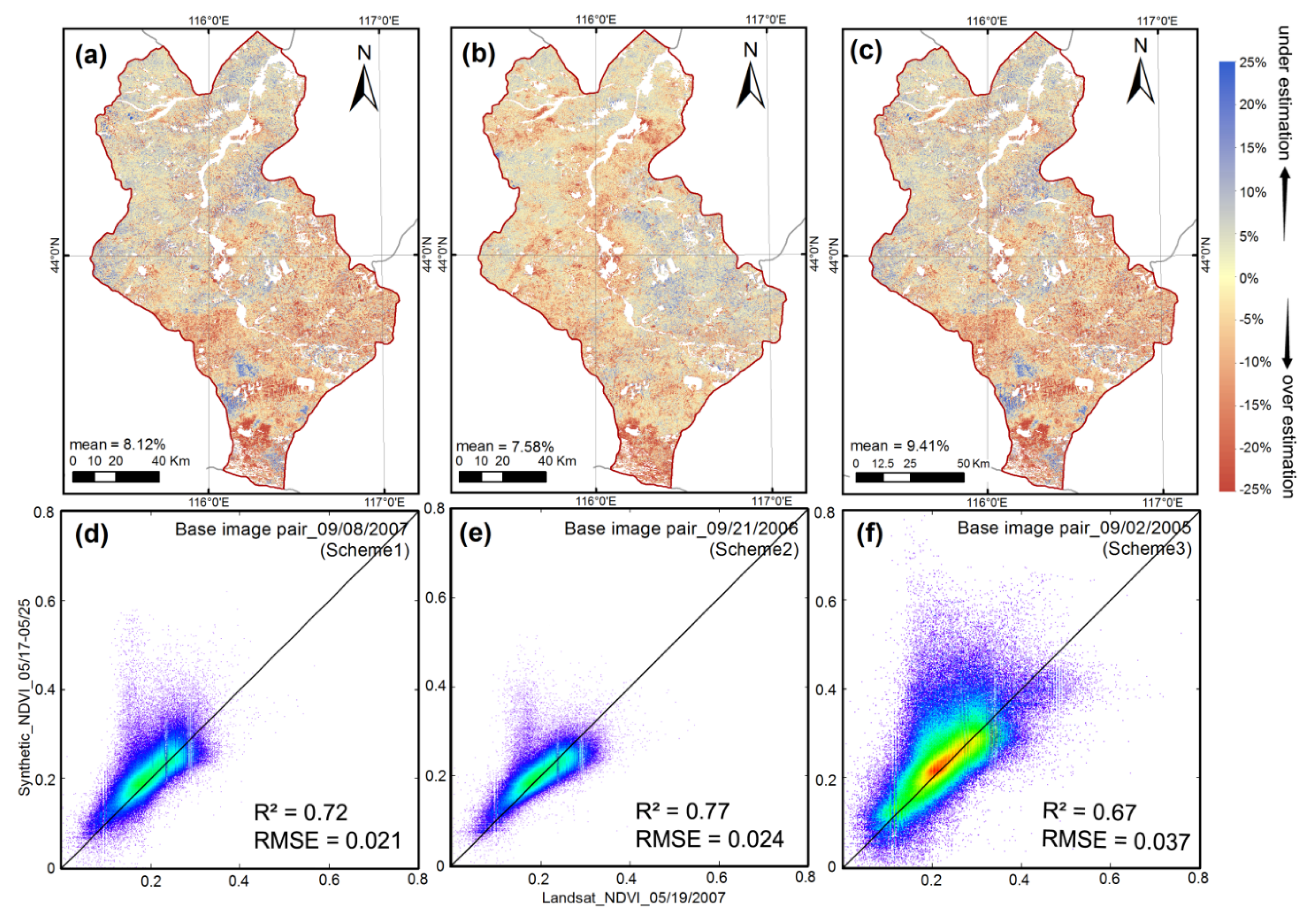
Figure 4 shows the validation results for the three fusion schemes described in Section 3.2, that is, data fusion within one year (Figure 4a,d) (2007), with adjacent years (Figure 4b,e) (2007 and 2006), and with 2-yr intervals (Figure 4c,f) (2007 and 2005). Red colors represent over-estimations and blue colors indicate under-estimations for synthetic NDVI. Figure 4d–f show the scatter plots between Landsat NDVI and synthetic NDVI for the three schemes. As we only considered grasslands in Xilinhot, all other vegetation types have been masked out.

There was good agreement between the observed Landsat NDVI images and synthetic NDVI data in the three schemes. The average relative errors between observed Landsat NDVI images and synthetic data were below 10% (8.12% for Scheme 1, 7.58% for Scheme 2, and 9.41% for Scheme 3). However, the pixels near lake shores, along riverbanks (mainly in the northern and central parts of the study area), and in other sparsely vegetated areas (mainly in the southern parts of the study area) showed larger differences between synthetic NDVI and NDVI derived from observed TM. The study of Zhang et al. [31] also pointed out that over-estimations of synthetic images were mainly located at pixels near riverbanks and lake shores in the mid-eastern parts of New Orleans, USA, and these were due to abrupt surface changes caused by urban flooding [31]. Cloud contamination can also cause bias between observed NDVI and synthetic NDVI [16]. Although the MODIS product used in this study give the 8-day optimal observations, it can still not fully remove the atmospheric noise [56], which could affect the accuracy of the fusion result. While in most of the study area, the grass sceneries were homogenous and the three schemes showed good fusion results. However, the fusion results of Scheme 1 (within one year) and Scheme 2 (with adjacent years) were slightly better than Scheme 3, as they had higher coefficients of determination (R²) and lower root-mean-square errors (R² = 0.72, RMSE = 0.021 for Scheme 1; R² = 0.77, RMSE = 0.024 for Scheme 2; R² = 0.67, RMSE = 0.037 for Scheme 3) (Figure 4).

Figure 4. Difference maps and scatter plots between the observed Landsat NDVI images (taken 19 May 2007) and the synthetic NDVI images (taken during 17–24 May 2007) predicted by (Left) (a,d) Scheme 1; (Middle) (b,e) Scheme 2, and (Right) (c,f) Scheme 3.

Figure 4. Difference maps and scatter plots between the observed Landsat NDVI images (taken 19 May 2007) and the synthetic NDVI images (taken during 17–24 May 2007) predicted by (Left) (a,d) Scheme 1; (Middle) (b,e) Scheme 2, and (Right) (c,f) Scheme 3.

We further chose five statistical indices (i.e., mean value, standard deviation, entropy, average gradient, and mean absolute difference) to assess the quality of the predicted synthetic NDVI products (Table 4). There were no considerable differences between the observed and predicted NDVI images for the three schemes, and the first four indices were nearly identical. The average differences were all below 0.025. In addition, the fused images in the same year (Scheme 1) and in the adjacent years had more consistent results with observed images than those from Scheme 3, as indicated by the five indices. In another woodland area, similar coefficient of determinations (0.66–0.94) between the observed TM NDVI and predicted NDVI were found by Bhandari et al. [23]. Overall, our predicted NDVI images were fairly reliable and could be used for accurate estimations of AGB. In the following work, we chose different data-fusion schemes according to the availability of TM images.

Table 4. Accuracy assessment of the fused images. TM_NDVI is the observed TM NDVI image and Pre_NDVI represents the predicted NDVI images at 30-m resolution that were derived from STARFM with Schemes 1, 2, and 3. Numbers in bold represent the best fit among the three schemes.

Type	Mean	Standard Deviation	Entropy	Average Gradient	Mean Absolute Difference
TM_NDVI	0.240	0.049	3.619	0.014	/
Pre_NDVI_Scheme1	0.244	0.053	3.653	0.013	0.019
Pre_NDVI_Scheme2	0.245	0.045	3.566	0.012	0.018
Pre_NDVI_Scheme3	0.247	0.060	3.725	0.016	0.022

Table 4. Accuracy assessment of the fused images. TM_NDVI is the observed TM NDVI image and Pre_NDVI represents the predicted NDVI images at 30-m resolution that were derived from STARFM with Schemes 1, 2, and 3. Numbers in bold represent the best fit among the three schemes.

Type	Mean	Standard Deviation	Entropy	Average Gradient	Mean Absolute Difference
TM_NDVI	0.240	0.049	3.619	0.014	/
Pre_NDVI_Scheme1	0.244	0.053	3.653	0.013	0.019
Pre_NDVI_Scheme2	0.245	0.045	3.566	0.012	0.018
Pre_NDVI_Scheme3	0.247	0.060	3.725	0.016	0.022

4.2. Prediction of Time-Series Synthetic NDVI

Based on the above analysis of the three fusion schemes, we decided to use data in the same year (except for 2008, 2012, and 2013), in adjacent years (2008, 2012), and data with 2-yr intervals (2013) (data shown in Table 1) to predict the synthetic NDVI.

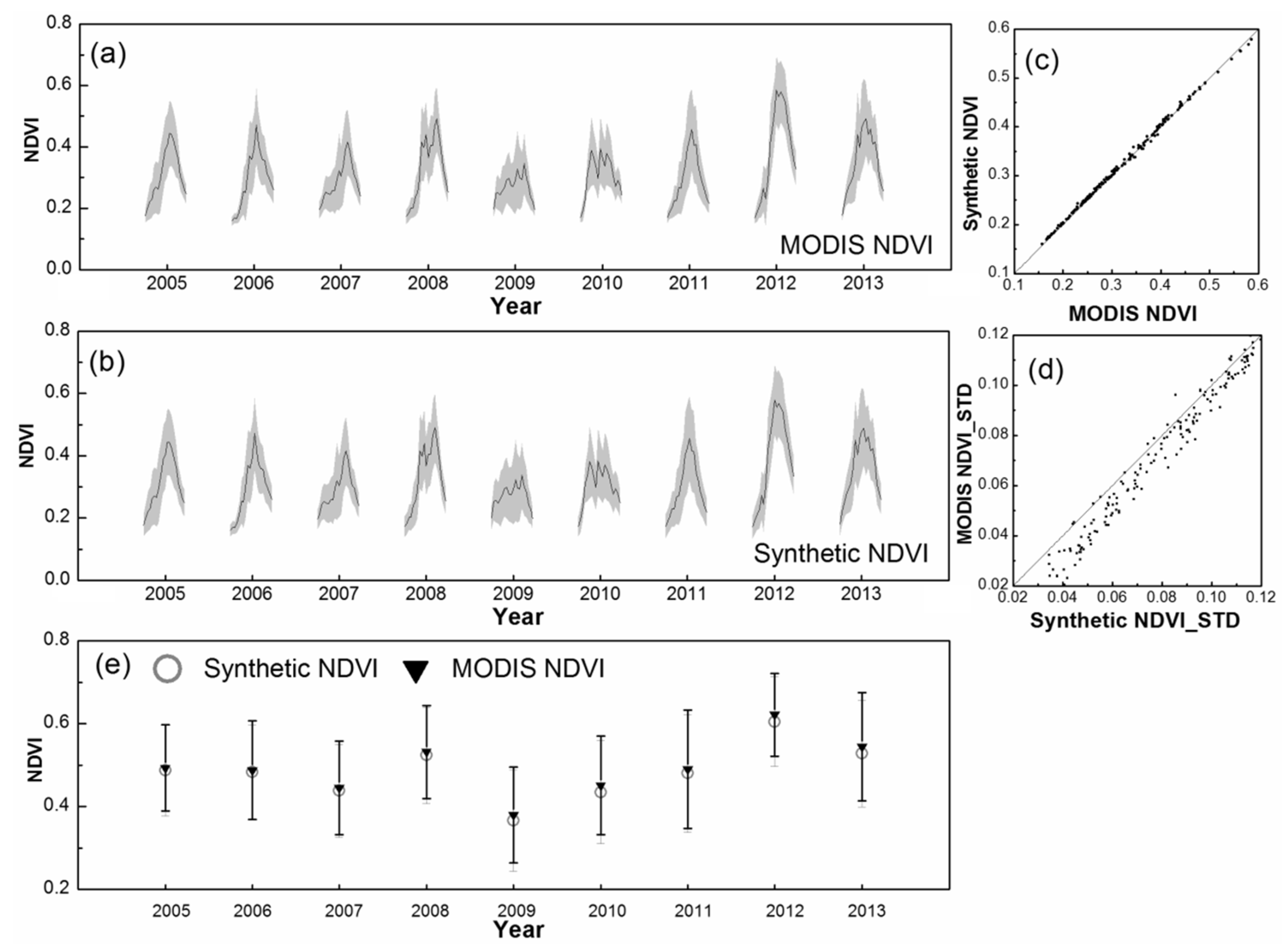
We fused TM and MODIS NDVI by using the STARFM method and predicted NDVI for each 8-d intervals during 2005–2013. A total of 180 NDVI scenes (20 scenes/yr for 9 yr) were predicted. Figure 5a,b show the mean and standard deviation of MODIS NDVI and synthetic NDVI at 8-day intervals during 2005–2013, respectively. Figure 5c shows the relationship between the MODIS NDVI and synthetic NDVI results that were shown in Figure 5a,b, respectively. Figure 5d shows the relationship between the standard deviations of the MODIS NDVI and synthetic NDVI results that were shown in Figure 5a,b, respectively. Figure 5e shows the maximum NDVI values of MODIS and synthetic images during the growing seasons, which represent the highest vegetation productivity within a year.

Figure 5. Temporal variations of the regional mean and standard deviation (shaded area) of NDVI for grasslands in the study areas during 2005–2013 (growing season). (a) MODIS NDVI; (b) synthetic NDVI; (c) scatter plots between MODIS NDVI and synthetic NDVI at 8-d intervals; (d) scatter plots between the standard deviation of MODIS NDVI and synthetic NDVI at 8-d intervals; (e) MODIS NDVI_max (black) and synthetic NDVI_max (gray). Error bars represent the standard deviations of MODIS NDVI_max (black) and synthetic NDVI_max (gray).

Figure 5. Temporal variations of the regional mean and standard deviation (shaded area) of NDVI for grasslands in the study areas during 2005–2013 (growing season). (a) MODIS NDVI; (b) synthetic NDVI; (c) scatter plots between MODIS NDVI and synthetic NDVI at 8-d intervals; (d) scatter plots between the standard deviation of MODIS NDVI and synthetic NDVI at 8-d intervals; (e) MODIS NDVI_max (black) and synthetic NDVI_max (gray). Error bars represent the standard deviations of MODIS NDVI_max (black) and synthetic NDVI_max (gray).

The means of the synthetic NDVI values were almost identical to those of the MODIS NDVI (Figure 5c). The predicted NDVI (30 m) therefore retained the high-frequency temporal information from the MODIS NDVI time series. The predicted images had larger standard deviations and represent larger dispersions of the imagery (Figure 5d), which indicates that the synthetic images may contain more detailed information. The differences between the standard deviation of MODIS NDVI and synthetic NDVI in this study were less than those reported in the study of Tian et al. [18]. In their study, these differences could be clearly observed in graphics similar to the ones in Figure 5a,b, and the shadow area of the synthetic NDVI series was much larger than the MODIS NDVI series. This can be explained by the homogeneous landscape for grasslands in Xilinhot, our study area. In contrast, in the study of Tian et al. [18], the study area was a mixed fragmentized landscape consisting of forests, shrublands, and residential areas.

Our results indicate that the accuracy of time-series NDVI derived from the STARFM algorithm was reliable and that the STARFM could effectively predict NDVI time series at higher spatial and temporal resolutions for the grasslands. The synthetic NDVI time series described more detailed spatial variations of NDVI at a resolution of 30 m. The temporal information from MODIS and the spatial information from Landsat were integrated in the predicted synthetic NDVI data set, and it was expected that such data can provide superior input for accurate estimations of AGB time series.

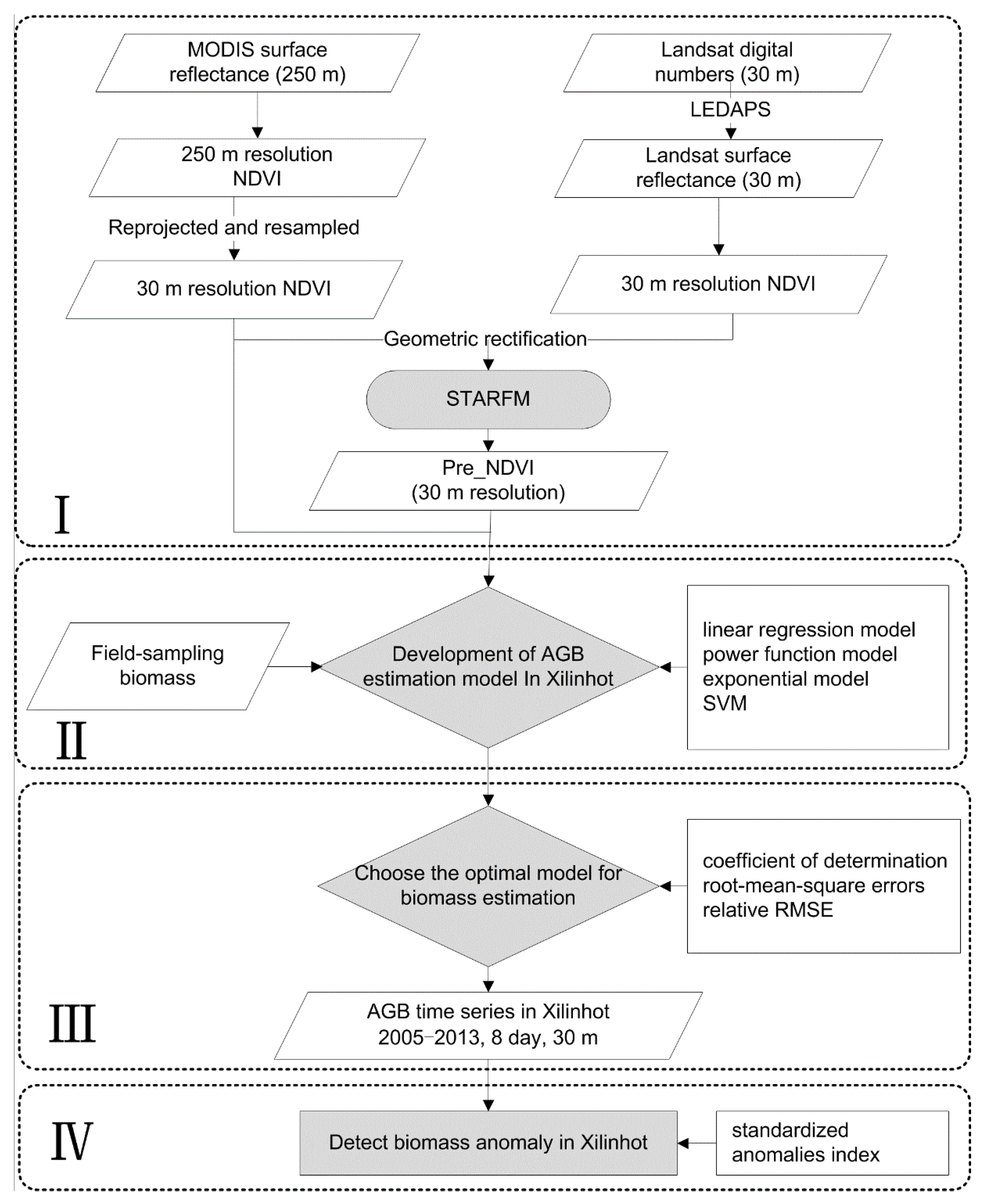
4.3. Development of the AGB Estimation Model

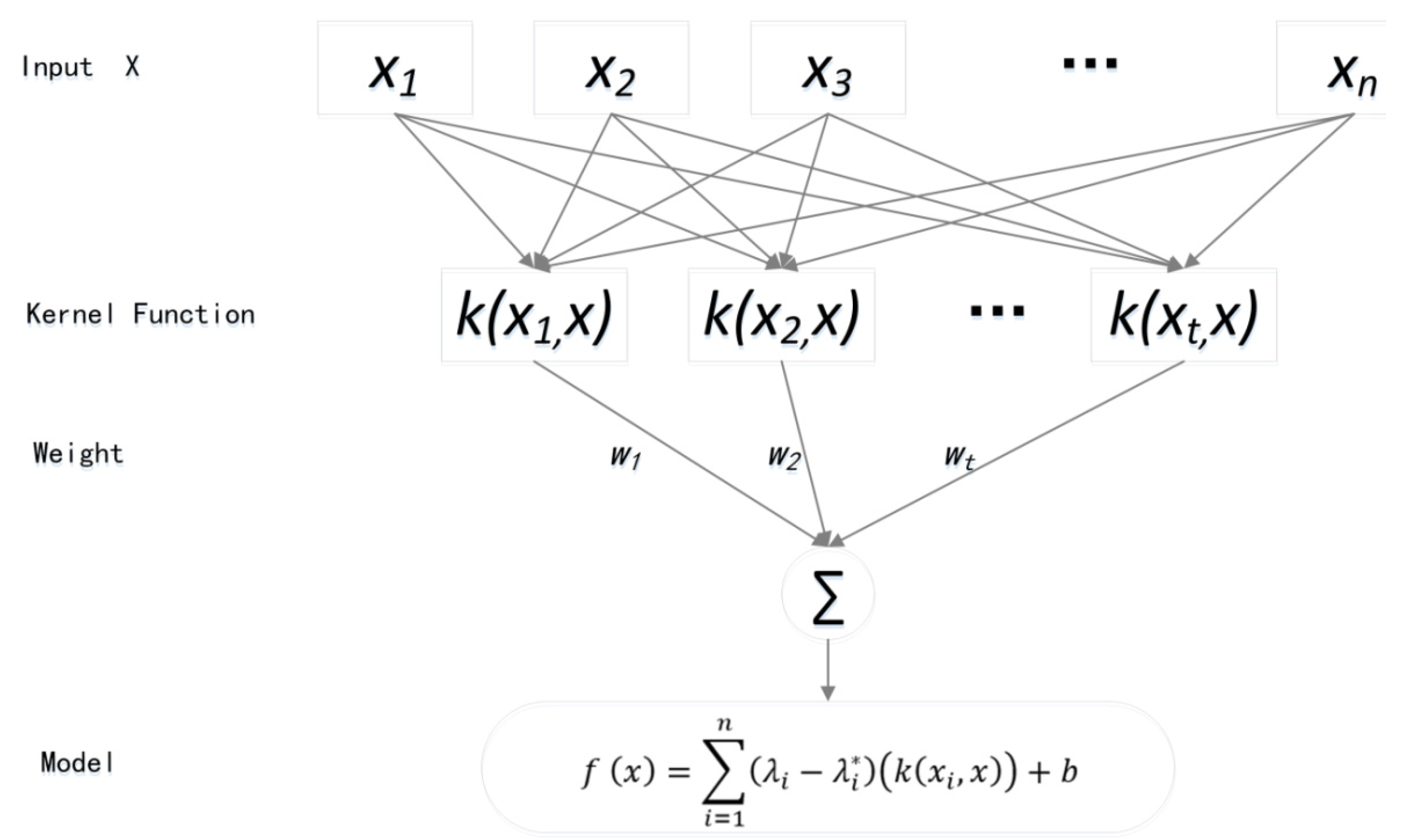
We developed four regression models for estimating the AGB, and these included linear regression model, power function model, exponential model, and support vector machine model (SVM-AGB). We randomly selected 46 biomass field samples and the corresponding synthetic NDVI pixels as the training set to construct the four models. We then used the other 22 samples to assess the accuracy of the four models. The accuracy assessment results indicated that for both MODIS NDVI and synthetic NDVI, the SVM-AGB model had higher accuracy than the other three models (Table 5 and Table 6). We further compared the synthetic NDVI-derived SVM-AGB model and MODIS NDVI-derived SVM-AGB model and found that the accuracies of the synthetic NDVI-derived SVM-AGB model data were higher than the accuracies of MODIS NDVI-derived SVM-AGB model data, as indicated by the R², RMSE, and RMSE_r for both the training set and testing set (Table 5 and Table 6). Therefore, we finally chose to integrate the SVM-AGB model and the synthetic NDVI to predict AGB for grasslands in Xilinhot during 2005–2013.

We compared our SVM-AGB model (R² = 0.77, RMSE = 17.22 g/m², RMSE_r = 24.8%) with other AGB estimation models in the same region, e.g., the exponential model based on 250-m MODIS NDVI (R² = 0.447) by Kawamura et al. [57]; the ANN model based on elevation, Landsat NDVI, and Landsat reflectance data (R² = 0.82, RMSE = 60.01 g/m², RMSE_r = 40.61%) by Xie et al. [35]; and the power function model based on 250-m MODIS NDVI (R² = 0.568, RMSE = 673.88 kg/ha) by Jin et al. [47]. The studies by Kawamura et al. [57] and Jin et al. [47] mainly used 250-m MODIS NDVI data, and the accuracies of their models were lower than that of our estimation model (R² = 0.447 by Kawamura et al.; R² = 0.568 by Jin et al.; R² = 0.77 by our synthetic NDVI-derived SVM-AGB model). Meanwhile, in the study of Xie et al. [35], although their ANN model was built on Landsat NDVI and reflectance images and possessed higher accuracy, the limitations of sparse temporal data associated with Landsat images restricted their model’s application to the requirements of frequent time series and dynamic monitoring. In general, our synthetic NDVI-derived SVM-AGB estimation model had both higher spatial resolutions (30 m) and temporal resolutions (8 d) than the other models in Table 5 and Table 6 and showed improvements compared to other AGB estimation models generated from a single type of remotely sensed data [33,35,47,56].

Table 5. Comparison of the accuracy of different AGB estimation models based on synthetic NDVI data.

AGB Model	Regression Equation	Training Set			Testing Set
		R2	RMSE	RMSEr	R2	RMSE	RMSEr
			(g/m2)			(g/m2)
Linear regression model	$\text{y}=2178 * x-1140$	0.71	31.40	42.6%	0.79	26.48	34.6%
Power function model	$\text{y}=1.044 * {10}^5 * x^{12.59}$	0.68	33.62	44.6%	0.84	28.03	38.0%
Exponential model	$\text{y}=3.902 * {10}^{-4} * e^{21.61 * x}$	0.67	34.14	45.1%	0.84	28.60	38.8%
SVM-AGB	/	0.77	17.22	24.8%	0.83	22.60	31.3%

Note: x represents synthetic NDVI; y represents AGB.

Table 5. Comparison of the accuracy of different AGB estimation models based on synthetic NDVI data.

AGB Model	Regression Equation	Training Set			Testing Set
		R2	RMSE	RMSEr	R2	RMSE	RMSEr
			(g/m2)			(g/m2)
Linear regression model	$\text{y}=2178 * x-1140$	0.71	31.40	42.6%	0.79	26.48	34.6%
Power function model	$\text{y}=1.044 * {10}^5 * x^{12.59}$	0.68	33.62	44.6%	0.84	28.03	38.0%
Exponential model	$\text{y}=3.902 * {10}^{-4} * e^{21.61 * x}$	0.67	34.14	45.1%	0.84	28.60	38.8%
SVM-AGB	/	0.77	17.22	24.8%	0.83	22.60	31.3%

Note: x represents synthetic NDVI; y represents AGB.

Table 6. Comparison of the accuracy of different AGB estimation models based on MODIS NDVI.

AGB Model	Regression Equation	Training Set			Testing Set
		R2	RMSE	RMSEr	R2	RMSE	RMSEr
			(g/m2)			(g/m2)
Linear regression model	$\text{y}=2010 * x-1043$	0.66	34.13	46.3%	0.64	34.19	42.1%
Power function model	$\text{y}=2.55 * {10}^5 * x^{14.15}$	0.68	33.21	44.8%	0.69	31.23	40.9%
Exponential model	$\text{y}=6.771 * {10}^{-5} * e^{\left(24.71 * x\right)}$	0.68	33.36	44.9%	0.69	31.24	41.1%
SVM-AGB	/	0.73	30.61	43.0%	0.72	22.89	37.1%

Note: x represents MODIS NDVI; y represents AGB.

Table 6. Comparison of the accuracy of different AGB estimation models based on MODIS NDVI.

AGB Model	Regression Equation	Training Set			Testing Set
		R2	RMSE	RMSEr	R2	RMSE	RMSEr
			(g/m2)			(g/m2)
Linear regression model	$\text{y}=2010 * x-1043$	0.66	34.13	46.3%	0.64	34.19	42.1%
Power function model	$\text{y}=2.55 * {10}^5 * x^{14.15}$	0.68	33.21	44.8%	0.69	31.23	40.9%
Exponential model	$\text{y}=6.771 * {10}^{-5} * e^{\left(24.71 * x\right)}$	0.68	33.36	44.9%	0.69	31.24	41.1%
SVM-AGB	/	0.73	30.61	43.0%	0.72	22.89	37.1%

Note: x represents MODIS NDVI; y represents AGB.

4.4. Drought Condition Monitoring with Time-Series Biomass Maps

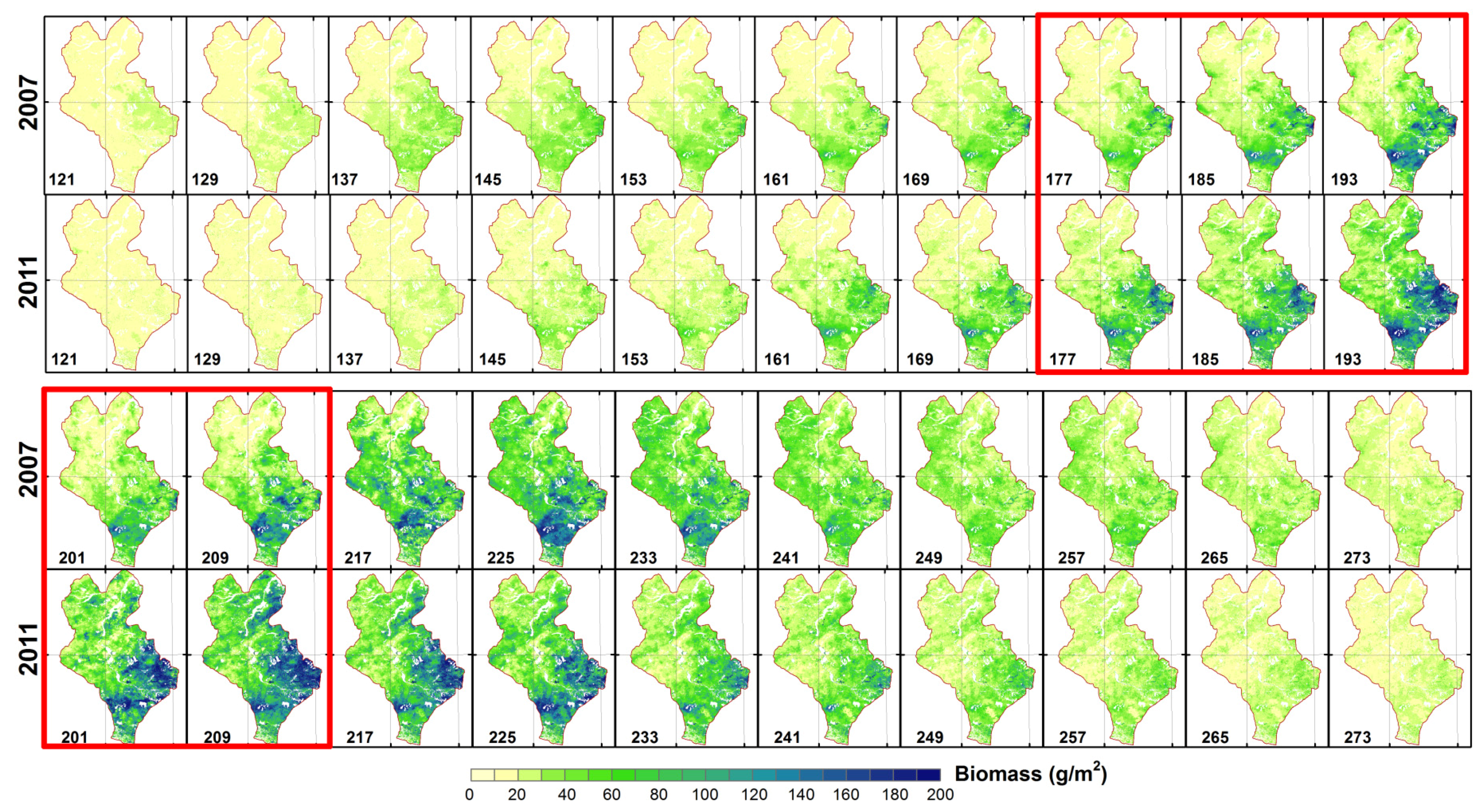
We further used all the 68 biomass field samples and the corresponding synthetic NDVI pixels to generate synthetic NDVI-derived SVM-AGB model. Specifically, we estimated the AGB for the entire grassland area of Xilinhot, Inner Mongolia, for the growing season during 2005–2013. Figure 6 illustrates the spatial distribution of biomass in 2007 (drought year) and 2011 (non-drought year) for each 8-d intervals during the growing season. 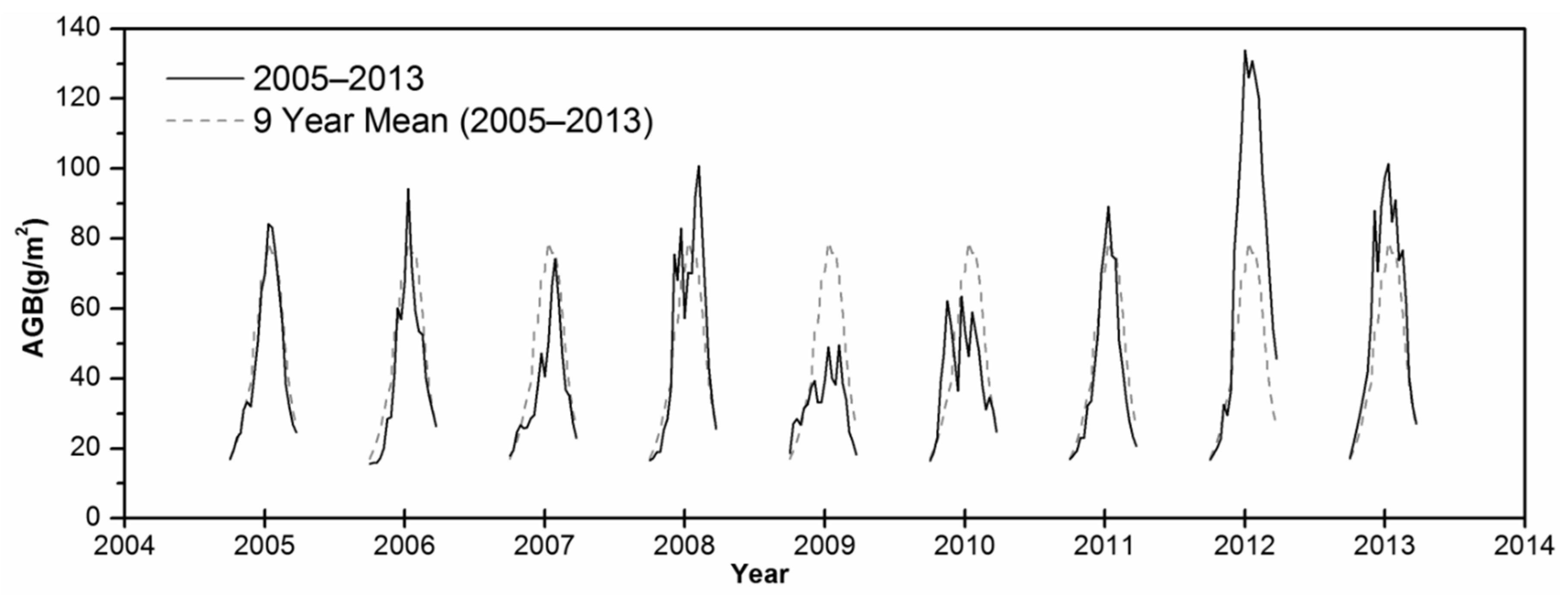Figure 7 shows the fluctuations of the regional mean biomass in the study areas during 2005–2013. The biomass variation of the regional mean in 2011 was almost identical with the 10-yr mean (Figure 7), and therefore, biomass maps in 2011 can be used to represent the general vegetation growth conditions in Xilinhot.

Generally, biomass for May–September exhibited large spatial heterogeneity, which is of great significance for detecting grassland conditions. The AGB generally showed a decreasing trend from the southeast to the northwest. In 2011, in the first week of May (day of year (DOY): 121), the grassland biomass was generally below 20 g/m² and the regional mean was 16.9 g/m². During July, nearly half of the grassland biomass values reached 40–50 g/m². Grassland biomass reached its peak values during the end of July and the start of August. In the last week of July (DOY: 209), the highest value reached to 190 g/m² in the southeast region, while in the northwest region, the biomass was as low as 35 g/m². Then, biomass started to decrease during the third week of August. In the first week of September (DOY: 233), the regional mean AGB was 34.0 g/m², and it decreased to 26.2 g/m² during the last week of September.

Figure 6. Spatial distribution of biomass in 2007 and 2011 for each 8-d intervals during the growing season.

Figure 6. Spatial distribution of biomass in 2007 and 2011 for each 8-d intervals during the growing season.

Figure 7. The 8-d intervals of the regional mean biomass estimated based on synthetic NDVI and SVM-AGB model during the growing season (May to September) of 2005–2013 in Xilinhot. Dash line represents the regional mean biomass of 9-yr mean (2005–2013).

Figure 7. The 8-d intervals of the regional mean biomass estimated based on synthetic NDVI and SVM-AGB model during the growing season (May to September) of 2005–2013 in Xilinhot. Dash line represents the regional mean biomass of 9-yr mean (2005–2013).

Returning to the drought analysis, comparisons of the biomass were made between 2007 (drought year) and 2011 (non-drought year). In 2007, biomass generally exhibited temporal variations similar to the biomass variations in 2011. Importantly, during the end of June to the end of July (DOY: 177–209) (indicated by red rectangles), large areas of biomass in 2007 showed much lower biomass compared with the biomass in 2011 (Figure 6), especially in the southwestern region of Xilinhot. During the third and fourth week of July (DOY: 201 and 209) in 2007, large areas of biomass in the southwest were below 100 g/m², while in 2011, the biomass values reached up to 150 g/m². For the remainder of the growing season, no large differences were detected between the biomass maps in 2007 and 2011.

Overall, the time series of biomass during the growing season of 2005–2013 (black line) generally showed similar temporal variations with the 9-yr mean (2005–2013) (dashed line) (Figure 7). However, biomass in 2007, 2009, and 2010 showed larger negative anomalies compared with the 9-yr means largely because of the droughts in this area.

The year of 2007 was recorded as a drought year [58], and the biomass values during June and October 2007 were mostly below the multi-year mean (Figure 7). This was consistent with the findings of Yu et al. [59] and Hang et al. [60]. Yu et al. [61] used the Modified Grassland Index (MGI) to monitor grassland variations in Xilingol (2001–2010) and found that the MGI values in 2007 were much lower than MGI values in other years. In the study of Hang et al. [60], the annual and seasonal NDVI in 2007 was below that in other years (2000–2010) in Xilingol. The largest negative biomass anomaly during 2005–2013 was found during the second week of July in 2009 (51.7% less than the 9-yr mean), followed by the second week of August in 2009 (50.0% lower than the 9-yr mean) and the first week of August in 2009 (47.0% lower than the 9-year mean). Jin et al. [47] also found that during 2006–2012, the biomass in 2009 was the lowest and it was 31.5% lower than the 7-yr mean in Xilingol League (Xilinhot is located in the center of Xilingol League). This was mainly attributed to severe drought and insect outbreaks in this region in 2009 [62]. Biomass in 2010 showed large fluctuations. According to the national grassland report in 2010 issued by Farmer’s daily [59], Xilingol League suffered from severe snow disasters during the end of 2009 and the beginning of 2010. For grasslands in Inner Mongolia, up to 32 million ha of grassland were affected [59], which could be a possible reason for the biomass fluctuations in 2010. Conversely, biomass in 2012 was much larger than that in other years. In the third week of July, the mean biomass of the study area even reached to 133.86 g/m², which was 88.9% higher than the 9-yr mean. Jin et al. [47] stated that 2012 was a prime harvest year for all of Xilingol, and the biomass value was 40% higher than the annual average (2005–2013) and twice the value in 2009.

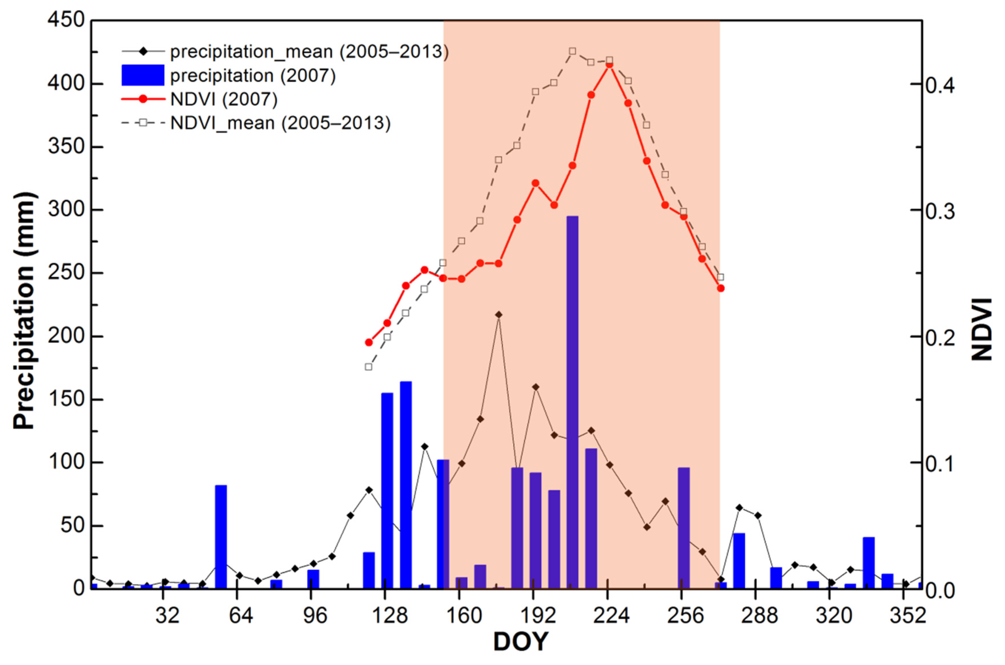
To further explore the capability of the synthetic NDVI for detecting anomalous vegetation activity, we took the biomass during the drought year (2007) as an example and then compared the data to the 9-yr mean (2005–2013) through using $SA{I}_{AGB}$. In 2007, large vegetation anomalies were mainly found during June to the start of August (Figure 8, DOY: 153–217), which can be attributed to the rainfall shortages. Large water deficiencies were detected during the start of March to the end of June (DOY: 64–176) (Figure 8). Other studies have found that precipitation has obvious lag effects on vegetation in the study region, and the lag response time is typically 48 to 56 d [61,63]. Although precipitation in the last week of July was even more than twice the 9-yr mean, it did not relieve the stress on vegetation during this month. Biomass in the third week of July in 2007 was even 42.7% lower than the multi-year mean (Figure 8).

Figure 8. Time series of precipitation and predicted synthetic NDVI (8-d intervals) for Xilinhot in 2007 (precipitation data at site Xilinhot were obtained from the China meteorological data sharing service system).

Figure 8. Time series of precipitation and predicted synthetic NDVI (8-d intervals) for Xilinhot in 2007 (precipitation data at site Xilinhot were obtained from the China meteorological data sharing service system).

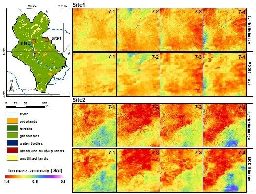
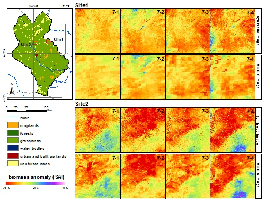
Figure 9 shows the biomass anomalies in 2007 compared with the mean of 2005–2013 during July. Site 1 was located at the Maodeng Ranch, which is China’s largest typical-steppe reserve [48]. Site 2 was occupied by lovely achnatherum, needlegrass, and little-leaf pea shrub [48]. The distribution of the biomass anomalies based on MODIS NDVI-derived biomass and synthetic NDVI-derived biomass data generally showed good agreement. However, the biomass derived from the synthetic NDVI image data showed more details compared with MODIS NDVI-derived biomass data. Terrain textures and roads can be clearly identified in the maps from the synthetic images. In addition, the absolute SAI of biomass maps from the synthetic NDVI images was generally larger than that of the MODIS NDVI-derived biomass images, which implies that the synthetic images can better capture the biomass anomalies than MODIS NDVI-derived biomass images.

Figure 9. The Standardized Anomalies Index (SAI) indicating biomass anomalies in Xilinhot during July 2007. The land cover map in Xilinhot in the left panel was adapted from the land cover data set provided by the Data Center for Resources and Environmental Sciences, Chinese Academy of Sciences (http://www.resdc.cn). The unutilized lands represent lands that have not been used (including desert, Gobi region, saline, wetlands, bare soil).

Figure 9. The Standardized Anomalies Index (SAI) indicating biomass anomalies in Xilinhot during July 2007. The land cover map in Xilinhot in the left panel was adapted from the land cover data set provided by the Data Center for Resources and Environmental Sciences, Chinese Academy of Sciences (http://www.resdc.cn). The unutilized lands represent lands that have not been used (including desert, Gobi region, saline, wetlands, bare soil).

5. Conclusions

Modeling aboveground biomass is of great importance to studies of grassland ecology and socio-economic environments in grassland regions. In order to predict biomass for grasslands with high spatial resolutions and temporal frequencies, we developed an aboveground biomass estimation model integrating synthetic NDVI data and the support vector machine technique (SVM-AGB). Our modeling method showed that the synthetic images can guarantee the accuracy of AGB estimations compared with AGB estimates from MODIS data (MODIS data: R² = 0.77 and RMSE = 17.22 g/m²; synthetic imagery: R² = 0.73 and RMSE = 30.61 g/m²). Importantly, the spatial-temporal resolution was improved (8 d, 30 m), which indicates that integrating the synthetic NDVI data and SVM model can produce accurate grassland AGB estimates for natural resource applications.

Based on the improved grassland AGB estimation model and synthetic NDVI, we mapped time-series AGB for grasslands of Xilinhot, Inner Mongolia, at 8-d intervals and 30-m resolutions. We successfully combined the STARFM and SVM into grassland biomass estimations. Compared with the biomass model using single data sources, our SVM-AGB model not only guarantees the accuracy of biomass estimations and achieves higher temporal frequencies, but it also improves the spatial resolution (i.e., from 250 to 30 m). Thus, it can capture biomass anomalies at finer scales, which is very useful for monitoring grassland conditions and conducting disaster assessments (such as during droughts). The high temporal (8 d) and medium spatial resolution (30 m) AGB estimations should be particularly useful for dynamic monitoring of grassland AGB, animal husbandry management, and general grassland management. Our approach can also be applied to grasslands in other geographical regions.

References

1. He, C.; Zhang, Q.; Li, Y.; Li, X.; Shi, P. Zoning grassland protection area using remote sensing and cellular automata modeling—A case study in Xilingol steppe grassland in northern China. J. Arid Environ. 2005, 63, 814–826. [Google Scholar] [CrossRef]
2. Jobbagy, E.G.; Sala, O.E. Controls of grass and shrub aboveground production in the Patagonian steppe. Ecol. Appl. 2000, 10, 541–549. [Google Scholar] [CrossRef]
3. Nordberg, M.L.; Evertson, J. Monitoring change in mountainous dry-heath vegetation at a regional scale using multitemporal Landsat TM data. Ambio 2003, 32, 502–509. [Google Scholar] [CrossRef] [PubMed]
4. Huete, A.; Didan, K.; Miura, T.; Rodriguez, E.P.; Gao, X.; Ferreira, L.G. Overview of the radiometric and biophysical performance of the MODIS vegetation indices. Remote Sens. Environ. 2002, 83, 195–213. [Google Scholar] [CrossRef]
5. Price, J.C. How unique are spectral signatures. Remote Sens. Environ. 1994, 49, 181–186. [Google Scholar] [CrossRef]
6. Asner, G.P. Cloud cover in Landsat observations of the Brazilian Amazon. Int. J. Remote Sens. 2001, 22, 3855–3862. [Google Scholar] [CrossRef]
7. Jorgensen, P.V. Determination of cloud coverage over Denmark using Landsat MSS/TM and NOAA–AVHRR. Int. J. Remote Sens. 2000, 21, 3363–3368. [Google Scholar] [CrossRef]
8. Ju, J.C.; Roy, D.P. The availability of cloud-free Landsat ETM plus data over the conterminous United States and globally. Remote Sens. Environ. 2008, 112, 1196–1211. [Google Scholar] [CrossRef]
9. Gur, E.; Zalevsky, Z. Resolution-enhanced remote sensing via multi spectral and spatial data fusion. Int. J. Image Data Fusion 2011, 2, 149–165. [Google Scholar] [CrossRef]
10. Carper, W.J.; Lillesand, T.M.; Kiefer, R.W. The use of intensity-hue-saturation transformations for merging SPOT panchromatic and multispectral image data. Photogramm. Eng. Remote. Sens. 1990, 56, 459–467. [Google Scholar]
11. Shettigara, V.K. A generalized component substitution technique for spatial enhancement of multispectral images using a higher resolution data set. Photogramm. Eng. Remote. Sens. 1992, 58, 561–567. [Google Scholar]
12. Yocky, D.A. Multiresolution wavelet decomposition image merger of Landsat thematic mapper and SPOT panchromatic data. Photogramm. Eng. Remote. Sens. 1996, 62, 1067–1074. [Google Scholar]
13. Fu, D.J.; Chen, B.Z.; Wang, J.; Zhu, X.L.; Hilker, T. An improved image fusion approach based on enhanced spatial and temporal the adaptive reflectance fusion model. Remote Sens. 2013, 5, 6346–6360. [Google Scholar] [CrossRef]
14. Gao, F.; Masek, J.; Schwaller, M.; Hall, F. On the blending of the Landsat and MODIS surface reflectance: Predicting daily Landsat surface reflectance. IEEE Trans. Geosci. Remote Sens. 2006, 44, 2207–2218. [Google Scholar]
15. Zhu, X.L.; Chen, J.; Gao, F.; Chen, X.H.; Masek, J.G. An enhanced spatial and temporal adaptive reflectance fusion model for complex heterogeneous regions. Remote Sens. Environ. 2010, 114, 2610–2623. [Google Scholar] [CrossRef]
16. Hilker, T.; Wulder, M.A.; Coops, N.C.; Seitz, N.; White, J.C.; Gao, F.; Masek, J.G.; Stenhouse, G. Generation of dense time series synthetic Landsat data through data blending with MODIS using a spatial and temporal adaptive reflectance fusion model. Remote Sens. Environ. 2009, 113, 1988–1999. [Google Scholar] [CrossRef]
17. Walker, J.J.; de Beurs, K.M.; Wynne, R.H.; Gao, F. Evaluation of Landsat and MODIS data fusion products for analysis of dryland forest phenology. Remote Sens. Environ. 2012, 117, 381–393. [Google Scholar] [CrossRef]
18. Tian, F.; Wang, Y.J.; Fensholt, R.; Wang, K.; Zhang, L.; Huang, Y. Mapping and evaluation of NDVI trends from synthetic time series obtained by blending Landsat and MODIS data around a coalfield on the Loess Plateau. Remote Sens. 2013, 5, 4255–4279. [Google Scholar] [CrossRef]
19. Schmidt, M.; Udelhoven, T.; Gill, T.; Roder, A. Long term data fusion for a dense time series analysis with MODIS and Landsat imagery in an Australian savanna. J. Appl. Remote Sens. 2012, 6, 063512. [Google Scholar]
20. Watts, J.D.; Powell, S.L.; Lawrence, R.L.; Hilker, T. Improved classification of conservation tillage adoption using high temporal and synthetic satellite imagery. Remote Sens. Environ. 2011, 115, 66–75. [Google Scholar] [CrossRef]
21. Singh, D. Generation and evaluation of gross primary productivity using Landsat data through blending with MODIS data. Int. J. Appl. Earth Obs. 2011, 13, 59–69. [Google Scholar] [CrossRef]
22. Singh, D. Evaluation of long-term NDVI time series derived from Landsat data through blending with MODIS data. Atmosfera 2012, 25, 43–63. [Google Scholar]
23. Bhandari, S.; Phinn, S.; Gill, T. Preparing Landsat image time series (LITS) for monitoring changes in vegetation phenology in Queensland, Australia. Remote Sens. 2012, 4, 1856–1886. [Google Scholar] [CrossRef]
24. Senf, C.; Leitao, P.J.; Pflugmacher, D.; van der Linden, S.; Hostert, P. Mapping land cover in complex Mediterranean landscapes using Landsat: Improved classification accuracies from integrating multi-seasonal and synthetic imagery. Remote Sens. Environ. 2015, 156, 527–536. [Google Scholar] [CrossRef]
25. Huang, B.; Song, H.H. Spatiotemporal reflectance fusion via sparse representation. IEEE Trans. Geosci. Remote Sens. 2012, 50, 3707–3716. [Google Scholar] [CrossRef]
26. Hilker, T.; Wulder, M.A.; Coops, N.C.; Linke, J.; McDermid, G.; Masek, J.G.; Gao, F.; White, J.C. A new data fusion model for high spatial and temporal-resolution mapping of forest disturbance based on Landsat and MODIS. Remote Sens. Environ. 2009, 113, 1613–1627. [Google Scholar] [CrossRef]
27. Gevaert, C.M.; García-Haro, F.J. A comparison of STARFM and an unmixing-based algorithm for Landsat and MODIS data fusion. Remote Sens. Environ. 2015, 156, 34–44. [Google Scholar] [CrossRef]
28. Shen, H.F.; Wu, P.H.; Liu, Y.L.; Ai, T.H.; Wang, Y.; Liu, X.P. A spatial and temporal reflectance fusion model considering sensor observation differences. Int. J. Remote Sens. 2013, 34, 4367–4383. [Google Scholar] [CrossRef]
29. Meng, J.H.; Du, X.; Wu, B.F. Generation of high spatial and temporal resolution NDVI and its application in crop biomass estimation. Int. J. Digit. Earth 2013, 6, 203–218. [Google Scholar] [CrossRef]
30. Huang, B.; Zhang, H.K. Spatio-temporal reflectance fusion via unmixing: Accounting for both phenological and land-cover changes. Int. J. Remote Sens. 2014, 35, 6213–6233. [Google Scholar] [CrossRef]
31. Zhang, F.; Zhu, X.L.; Liu, D.S. Blending MODIS and Landsat images for urban flood mapping. Int. J. Remote Sens. 2014, 35, 3237–3253. [Google Scholar] [CrossRef]
32. Emelyanova, I.V.; McVicar, T.R.; van Niel, T.G.; Li, L.T.; van Dijk, A.I.J.M. Assessing the accuracy of blending Landsat-MODIS surface reflectances in two landscapes with contrasting spatial and temporal dynamics: A framework for algorithm selection. Remote Sens. Environ. 2013, 133, 193–209. [Google Scholar] [CrossRef]
33. Gao, T.; Xu, B.; Yang, X.C.; Jin, Y.X.; Ma, H.L.; Li, J.Y.; Yu, H.D. Using MODIS time series data to estimate aboveground biomass and its spatio-temporal variation in Inner Mongolia’s grassland between 2001 and 2011. Int. J. Remote Sens. 2013, 34, 7796–7810. [Google Scholar] [CrossRef]
34. Tomppo, E.; Nilsson, M.; Rosengren, M.; Aalto, P.; Kennedy, P. Simultaneous use of Landsat-TM and IRS-1C WIFS data in estimating large area tree stem volume and aboveground biomass. Remote Sens. Environ. 2002, 82, 156–171. [Google Scholar] [CrossRef]
35. Xie, Y.C.; Sha, Z.Y.; Yu, M.; Bai, Y.F.; Zhang, L. A comparison of two models with Landsat data for estimating above ground grassland biomass in Inner Mongolia, China. Ecol. Model 2009, 220, 1810–1818. [Google Scholar] [CrossRef]
36. Jin, Y.Q.; Liu, C. Biomass retrieval from high-dimensional active/passive remote sensing data by using artificial neural networks. Int. J. Remote Sens. 1997, 18, 971–979. [Google Scholar] [CrossRef]
37. Uno, Y.; Prasher, S.O.; Lacroix, R.; Goel, P.K.; Karimi, Y.; Viau, A.; Patel, R.M. Artificial neural networks to predict corn yield from compact airborne spectrographic imager data. Comput. Electron. Agric. 2005, 47, 149–161. [Google Scholar] [CrossRef]
38. Yool, S.R. Land cover classification in rugged areas using simulated moderate-resolution remote sensor data and an artificial neural network. Int. J. Remote Sens. 1998, 19, 85–96. [Google Scholar] [CrossRef]
39. Ban, Y.F. Synergy of multitemporal ERS-1 SAR and Landsat TM data for classification of agricultural crops. Can. J. Remote Sens. 2003, 29, 518–526. [Google Scholar] [CrossRef]
40. Erbek, F.S.; Ozkan, C.; Taberner, M. Comparison of maximum likelihood classification method with supervised artificial neural network algorithms for land use activities. Int. J. Remote Sens. 2004, 25, 1733–1748. [Google Scholar] [CrossRef]
41. Mathur, P.; Govil, R. Detecting temporal changes in satellite imagery using ANN. In Proceedings of the RAST 2005 2nd International Conference on Recent Advances in Space Technologies, Istanbul, Turkey, 9–11 June 2005; pp. 645–647.
42. Balabin, R.M.; Lomakina, E.I. Support vector machine regression (SVR/lS-SVM)—An alternative to neural networks (ANN) for analytical chemistry? Comparison of nonlinear methods on near infrared (NIR) spectroscopy data. Analyst 2011, 136, 1703–1712. [Google Scholar] [CrossRef] [PubMed]
43. Chen, G.; Hay, G.J.; Zhou, Y.L. Estimation of forest height, biomass and volume using support vector regression and segmentation from Lidar transects and Quickbird imagery. In Proceedings of the 2010 18th International Conference on Geoinformatics, Beijing, China, 18–20 June 2010; pp. 1–4.
44. Gleason, C.J.; Im, J. Forest biomass estimation from airborne LiDAR data using machine learning approaches. Remote Sens. Environ. 2012, 125, 80–91. [Google Scholar] [CrossRef]
45. Jachowski, N.R.A.; Quak, M.S.Y.; Friess, D.A.; Duangnamon, D.; Webb, E.L.; Ziegler, A.D. Mangrove biomass estimation in southwest Thailand using machine learning. Appl. Geogr. 2013, 45, 311–321. [Google Scholar] [CrossRef]
46. Tu, Y. Based on Meteorological Data of Drought Disaster Forecast Study in Pastoral Area of Xilingol League. Master’s Thesis, Inner Mongolia Normal University, Hohhot, China, 2013. [Google Scholar]
47. Jin, Y.X.; Yang, X.C.; Qiu, J.J.; Li, J.Y.; Gao, T.; Wu, Q.; Zhao, F.; Ma, H.L.; Yu, H.D.; Xu, B. Remote sensing-based biomass estimation and its spatio-temporal variations in temperate grassland, northern china. Remote Sens. 2014, 6, 1496–1513. [Google Scholar] [CrossRef]
48. Guan, L.L.; Liu, L.Y.; Peng, D.L.; Hu, Y.; Jiao, Q.J.; Liu, L.L. Monitoring the distribution of C3 and C4 grasses in a temperate grassland in northern China using moderate resolution imaging spectroradiometer normalized difference vegetation index trajectories. J. Appl. Remote Sens. 2012, 6. [Google Scholar] [CrossRef]
49. Masek, J.G.; Vermote, E.F.; Saleous, N.E.; Wolfe, R.; Hall, F.G.; Huemmrich, K.F.; Gao, F.; Kutler, J.; Lim, T.K. A Landsat surface reflectance dataset for North America, 1990–2000. IEEE Geosci. Remote Sens. Lett. 2006, 3, 68–72. [Google Scholar] [CrossRef]
50. Bai, Y.F.; Han, X.G.; Wu, J.G.; Chen, Z.Z.; Li, L.H. Ecosystem stability and compensatory effects in the Inner Mongolia grassland. Nature 2004, 431, 181–184. [Google Scholar] [CrossRef] [PubMed]
51. Vermonte, E.F.; Kotchenova, S.Y.; Ray, J.P. MODIS Surface Reflectance User’s Guide, Version 1.4. Available online: http://modis-sr.ltdri.org/guide/MOD09_UserGuide_v1_3.pdf (accessed on 16 November 2015).
52. Makela, H.; Pekkarinen, A. Estimation of forest stand volumes by Landsat TM imagery and stand-level field-inventory data. For. Ecol. Manag. 2004, 196, 245–255. [Google Scholar] [CrossRef]
53. Katz, R.W.; Glantz, M.H. Anatomy of a rainfall index. Mon. Weather Rev. 1986, 114, 764–771. [Google Scholar] [CrossRef]
54. Jarihani, A.A.; McVicar, T.R.; van Niel, T.G.; Emelyanova, I.V.; Callow, J.N.; Johansen, K. Blending Landsat and MODIS data to generate multispectral indices: A comparison of “Index-then-blend”and “Blend-then-index” approaches. Remote Sens. 2014, 6, 9213–9238. [Google Scholar] [CrossRef] [Green Version]
55. Hsu, C.W.; Chang, C.C.; Lin, C.J. A Practical Guide to Support Vector Classification. Available online: https://www.csie.ntu.edu.tw/~cjlin/papers/guide/guide.pdf (accessed on 19 November 2015).
56. Rembold, F.; Atzberger, C.; Savin, I.; Rojas, O. Using low resolution satellite imagery for yield prediction and yield anomaly detection. Remote Sens. 2013, 5, 1704–1733. [Google Scholar] [CrossRef] [Green Version]
57. Kawamura, K.; Akiyama, T.; Yokota, H.; Tsutsumi, M.; Yasuda, T.; Watanabe, O.; Wang, S.P. Quantifying grazing intensities using geographic information systems and satellite remote sensing in the Xilingol steppe region, Inner Mongolia, China. Agric. Ecosyst. Environ. 2005, 107, 83–93. [Google Scholar] [CrossRef]
58. Chun, F.; Li, C.L.; Bao, Y.H. The wavelet analysis of average temperature and precipitation in Xilinhot during 57 years. J. Inner Mong. Normal Univ. (Nat. Sci. Ed.) 2013, 42, 47–52. (In Chinese) [Google Scholar]
59. Farmer's Daily. Available online: http://szb.farmer.com.cn/nmrb/html/2011–04/13/nw.D110000nmrb_20110413_1–03.htm?div=-1 (accessed on 4 September 2015).
60. Hang, Y.L.; Bao, G.; Bao, Y.H.; Burenjirigala; Altantuya, D. Spatiotemporal changes of vegetation coverage in Xilingol grassland and its responses to climate change during 2000–2010. Acta Agres. Sin. 2014, 22, 1194–1204. (In Chinese) [Google Scholar]
61. Yu, H.D.; Yang, X.C.; Xu, B.; Jin, Y.X.; Gao, T.; Li, J.Y. Changes of grassland vegetation growth in Xilingol league over 10 years and analysis on the influence factors. J. Geo-Inf. Sci. 2013, 15, 270–279. (In Chinese) [Google Scholar]
62. Xilinhaote News. Available online: http://xilinhaote.nmgnews.com.cn/system/2009/07/20/010253966.shtml (accesed on 4 September 2015).
63. Liu, C.L.; Fan, R.H.; Wu, J.J.; Yan, F. Temporal lag of grassland vegetation growth response to precipitation in Xilinguolemeng. Arid Land Geogr. 2009, 32, 512–518. (In Chinese) [Google Scholar]