
High-Resolution Mapping of Urban Surface Water Using ZY-3 Multi-Spectral Imagery

 ,
,
Abstract
:
1. Introduction
2. Study Areas and Data
2.1. Study Area

| City’s Name and Location | Image Size (pixels) | Water Types | Topography | Climate | Color Infrared Composite | |
|---|---|---|---|---|---|---|
| Qingdao (36.2°N, 120.5°E) | 4574 × 5992 (922.0 km2) | Rivers Lakes Sea Harbors Reservoirs Ponds Aquatic parks | Basin, plain, hills, etc. | Warm temperate monsoon climate |  | |
| Aksu (41.4°N, 80.2°E) | 894 × 661 (19.9 km2) | Narrow clear river Narrow turbid river | Basin | Temperate continental arid climate |  | |
| Fuzhou (25.9°N, 119.3°E) | 1437 × 983 (47.5 km2) | Clear reservoirs Eutrophic reservoirs Clear man-made lake | Basin and hill | Subtropical monsoon climate |  | |
| Wuhan (30.7°N, 114.4°E) | Hanyang | 1135 × 658 (25.1 km2) | Polluted lakes | Plain | Subtropical monsoon humid climate |  |
| Huangpo | 1430 × 1112 (50.1 km2) | Clear ponds Eutrophic ponds Big clear river Big clear lake |  | |||
| Huainan (32.7°N, 116.9°E) | 1037 × 659 (23.0 km2) | Clear aquatic parks | Plain | Temperate monsoon climate |  | |
2.2. ZY-3 Multi-Spectral Imagery
| Experiment Sites | ZY-3 Scene | Reference Data and Sources | |||
|---|---|---|---|---|---|
| Acquisition Date | Path | Row | Solar Azimuth | ||
| Water bodies in Qingdao, Shandong | 17 October 2012 | 885 | 133 | 47.1 | Google Earth™ image acquired on 5–19 September. 2012 ©CNES/Astrium |
| Rivers in Aksu, Xinjiang | 22 October 2013 | 93 | 120 | 36.7 | Google Earth™ image acquired on 2 October 2013 ©CNES/Astrium |
| Reservoirs in Fuzhou, Fujian | 9 May 2013 | 881 | 159 | 42.6 | Google Earth™ image acquired on 16 Janaury 2013 © DigitalGlobe |
| Polluted lakes, fishponds in Wuhan, Hubei | 12 August 2013 | 897 | 147 | 67.6 | Google Earth™ image acquired on 16 August and 29 September 2013 © DigitalGlobe |
| Water bodies in Huainan, Anhui | 4 November 2013 | 892 | 142 | 40.7 | Google Earth™ image acquired on 2 October 2013 © DigitalGlobe |
2.3. Reference Data
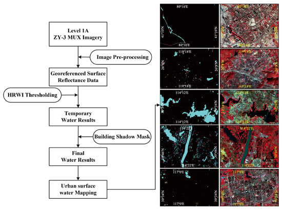
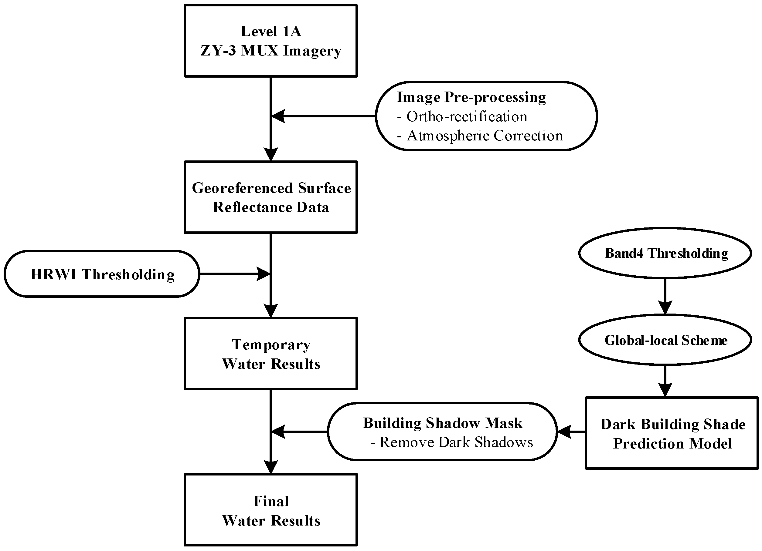
3. Method
3.1. Image Preprocessing
3.2. Formulation of the High Resolution Water Index (HRWI)
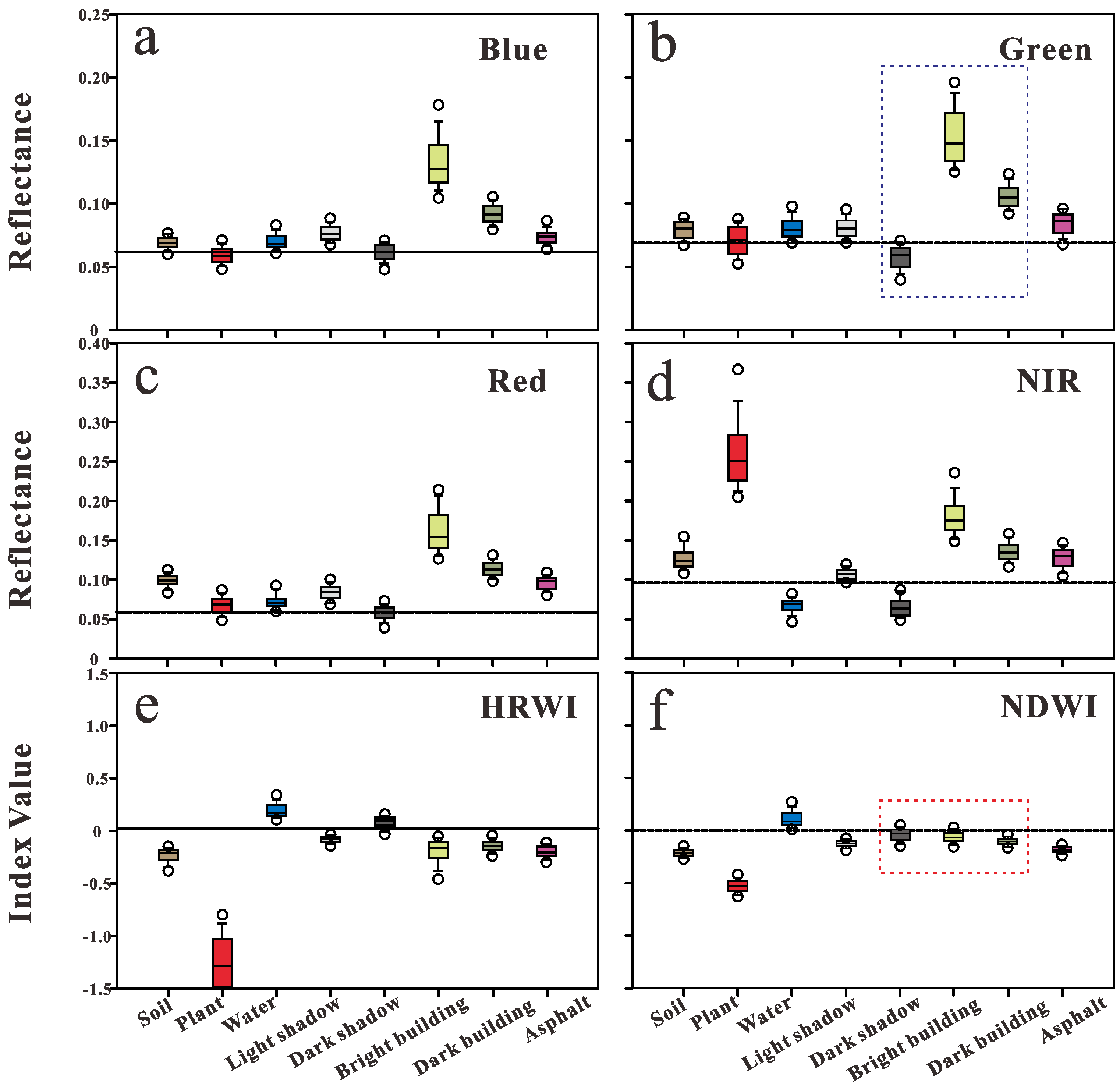
3.2.1. Index Model Selection
3.2.2. Band Selection
3.2.3. Coefficient Calculation
- are the training sample vectors,
- stands for the corresponding class label,
- is the kernel function,
- C is a constant.
- w is the normal vector which is perpendicular to the hyperplane,
- x is a three-dimensional vector composed of reflectance values from green, red and NIR bands,
- b is the intercept term.
- is the difference in the means of the water and other land cover type,
- is the sum of the standard deviations.
| Pair Comparison | M | ||
|---|---|---|---|
| HRWI | NDWI | Difference (HRWI-NDWI) | |
| Water vs. Bright building | 1.91 | 1.28 | 0.63 |
| Water vs. Dark building | 2.26 | 0.50 | 1.76 |
| Water vs. Asphalt | 2.56 | 2.08 | 0.48 |
| Water vs. Light shadow | 2.23 | 1.72 | 0.52 |
| Water vs. Dark shadow | 1.08 | 1.11 | −0.03 |
| Water vs. Soil | 2.55 | 2.16 | 0.39 |
| Water vs. Vegetation | 3.30 | 3.43 | −0.13 |
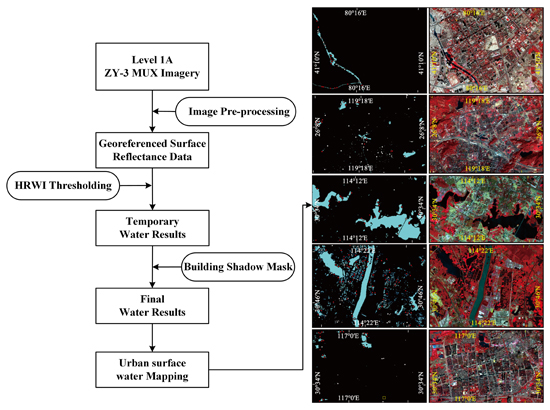
3.3. Automated Building Shadow Detection Method
3.3.1. Spatial Relationship between a Building and Its Shadow
3.3.2. Spectral Characteristics of Buildings and Shadows

3.3.3. Generating a Dark Building Shadow Prediction Model
| City | NSWB | NDSB | NCPB | OA (%) | Kappa |
|---|---|---|---|---|---|
| Qingdao | 82 | 106 | 181 | 96.28 | 0.92 |
| Fuzhou | 71 | 168 | 223 | 93.31 | 0.85 |
| Huainan | 105 | 136 | 228 | 94.61 | 0.89 |
| Wuhan | 73 | 202 | 262 | 95.27 | 0.88 |
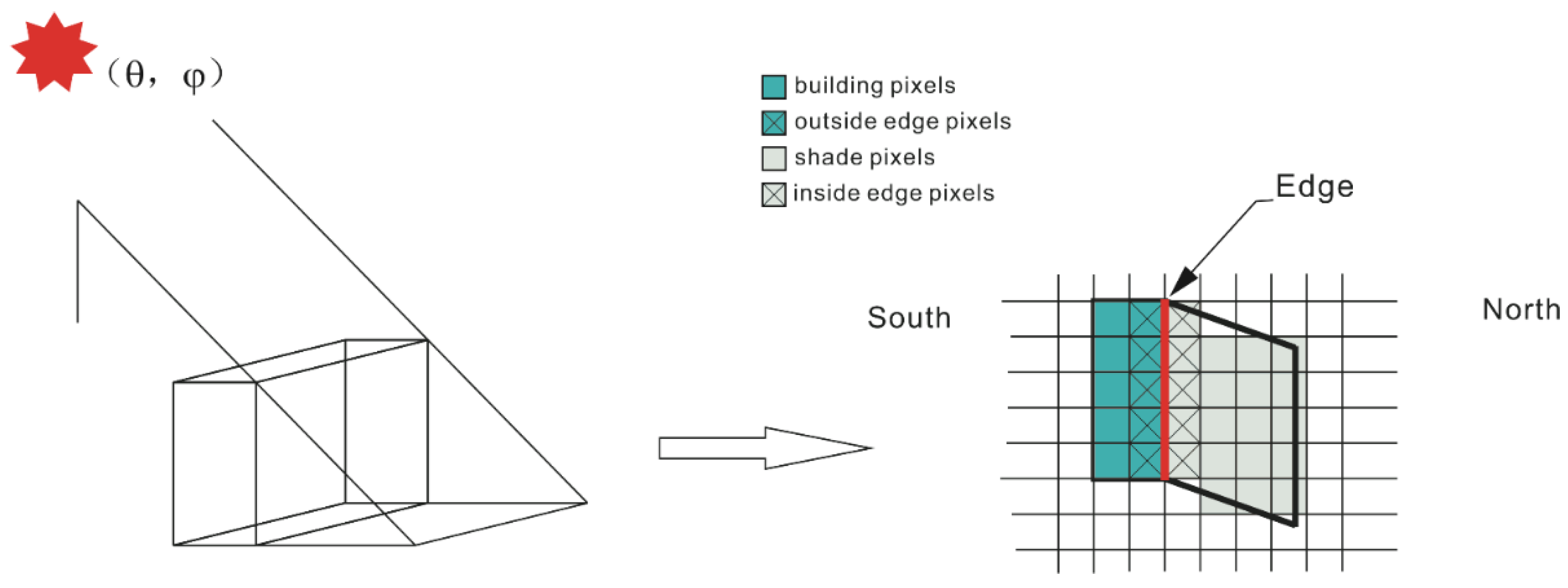
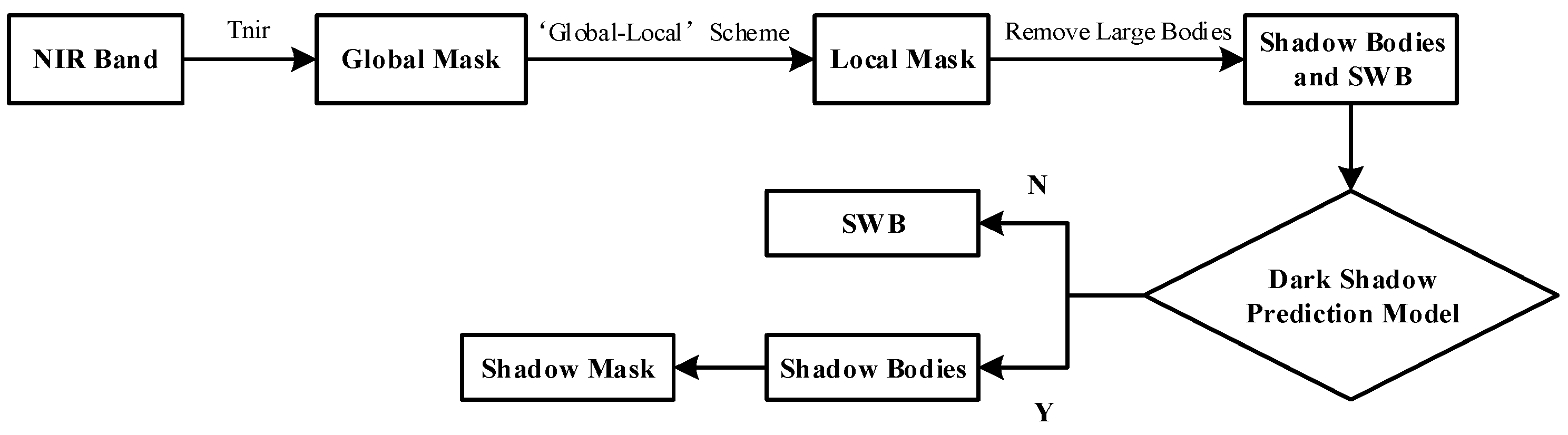
3.3.4. Automated Dark Building Shadow Detection Method

3.4. Urban Water Extraction Method and Accuracy Assessment
| Test Site | Aksu | Fuzhou | Hanyang | Huangpo | Huainan |
|---|---|---|---|---|---|
| Number of verification pixels | 29,988 | 20,000 | 5000 | 10,000 | 30,000 |

4. Results
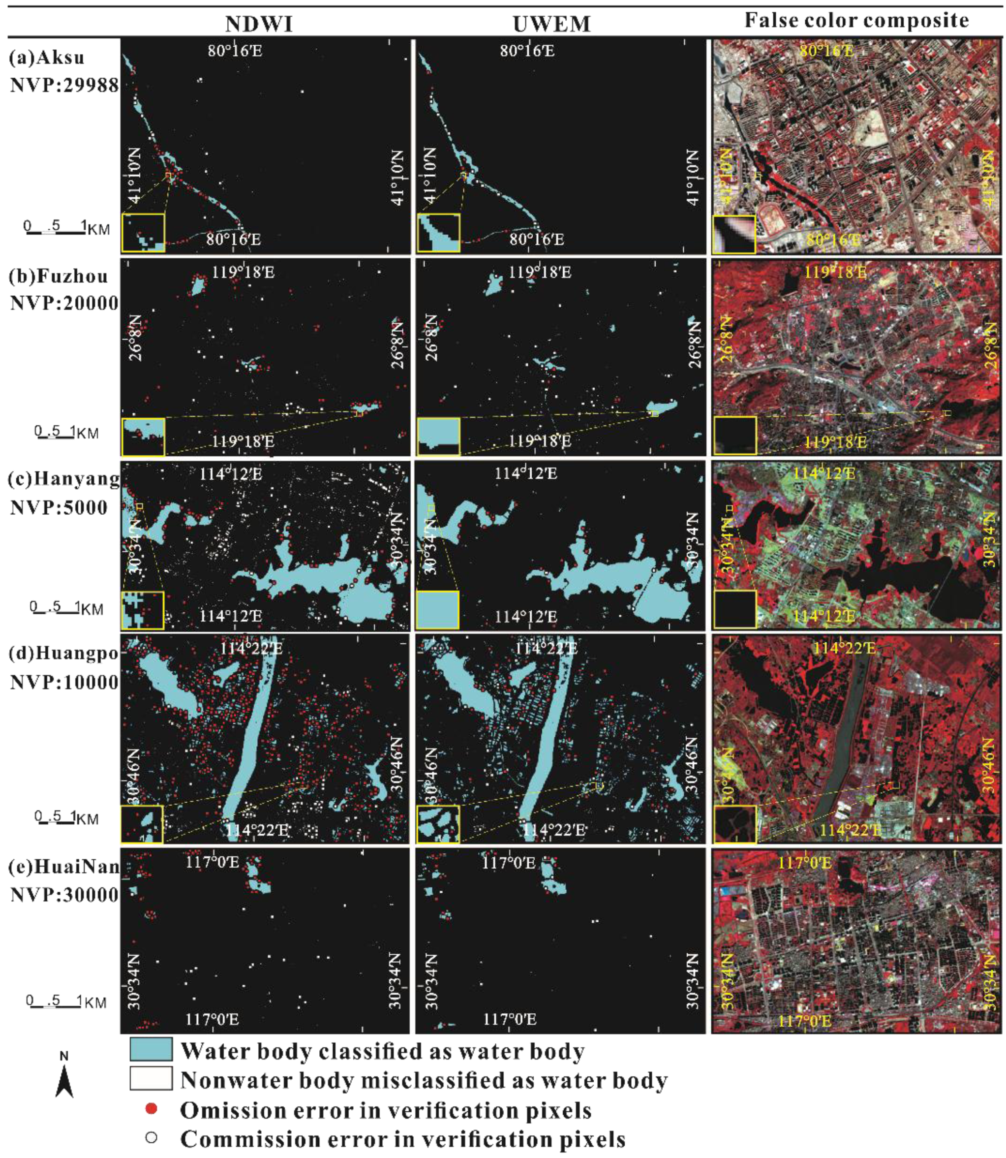
4.1. Water Extraction Maps

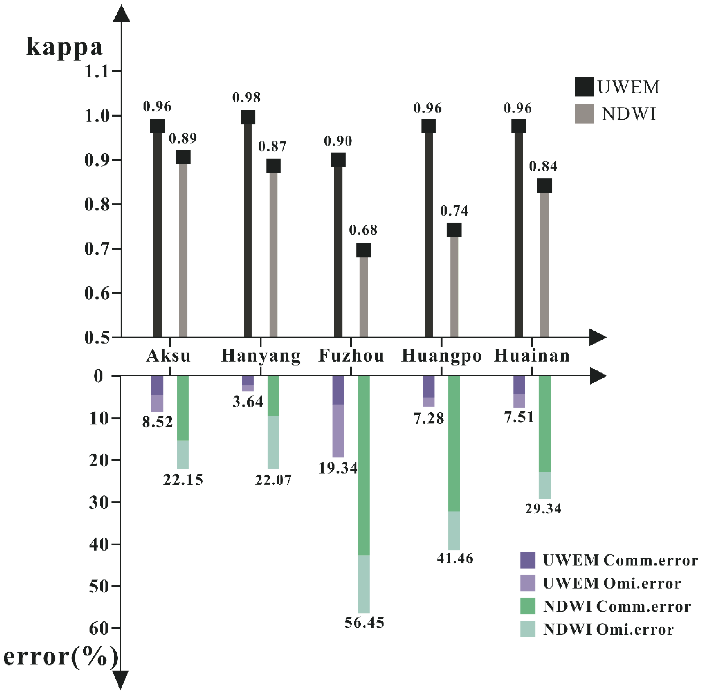
4.2. Water Extraction Accuracy
4.3. Threshold’s Stability
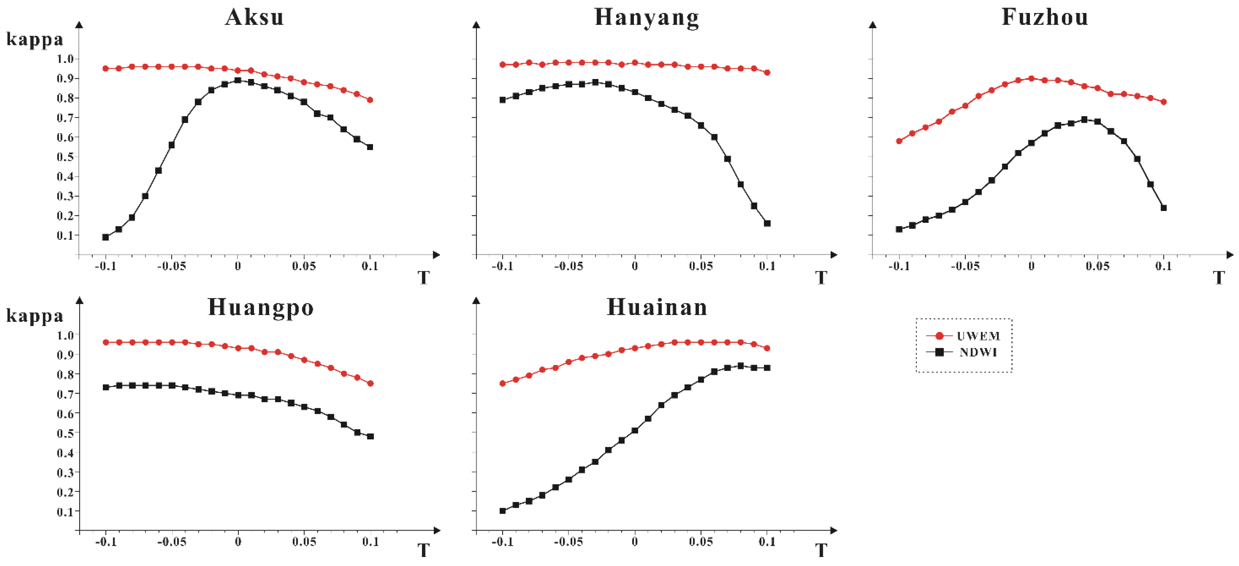
| Method | Range | Aksu | Hanyang | Fuzhou | Huangpo | Huainan |
|---|---|---|---|---|---|---|
| STD(Kappa) | STD(Kappa) | STD(Kappa) | STD(Kappa) | STD(Kappa) | ||
| UWEM | [−0.05, 0.05] | 0.027 | 0.008 | 0.042 | 0.029 | 0.036 |
| NDWI | [−0.05, 0.05] | 0.098 | 0.075 | 0.153 | 0.034 | 0.176 |
| UWEM | [−0.1, 0.1] | 0.052 | 0.013 | 0.095 | 0.067 | 0.069 |
| NDWI | [−0.1, 0.1] | 0.257 | 0.215 | 0.197 | 0.082 | 0.269 |
5. Discussion
- For the shortcomings of ratio model, the coefficient model is a better choice to develop a water index, because it can better reflect the differences of spectral characteristics between water and other surface features.
- Unlike the general empirical algorithms [11], there are two prominent advantages in the coefficient model developed with SVM: the inherent default threshold of the index is zero; the index can achieve the largest separation between water and other land cover types. Therefore, SVM is an outstanding method for training coefficient index. This study provides a potential method for remote sensing researchers to develop a suitable water index using the coefficient model, which is of great significance to relative studies in the future.
- To reduce the commission errors caused by dark shadow, a dark building shadow prediction model was proposed using two spectral variables as inputs. These two variables combine the spectral characteristics of a building and its shadow, making the model keep both good separation and stability.
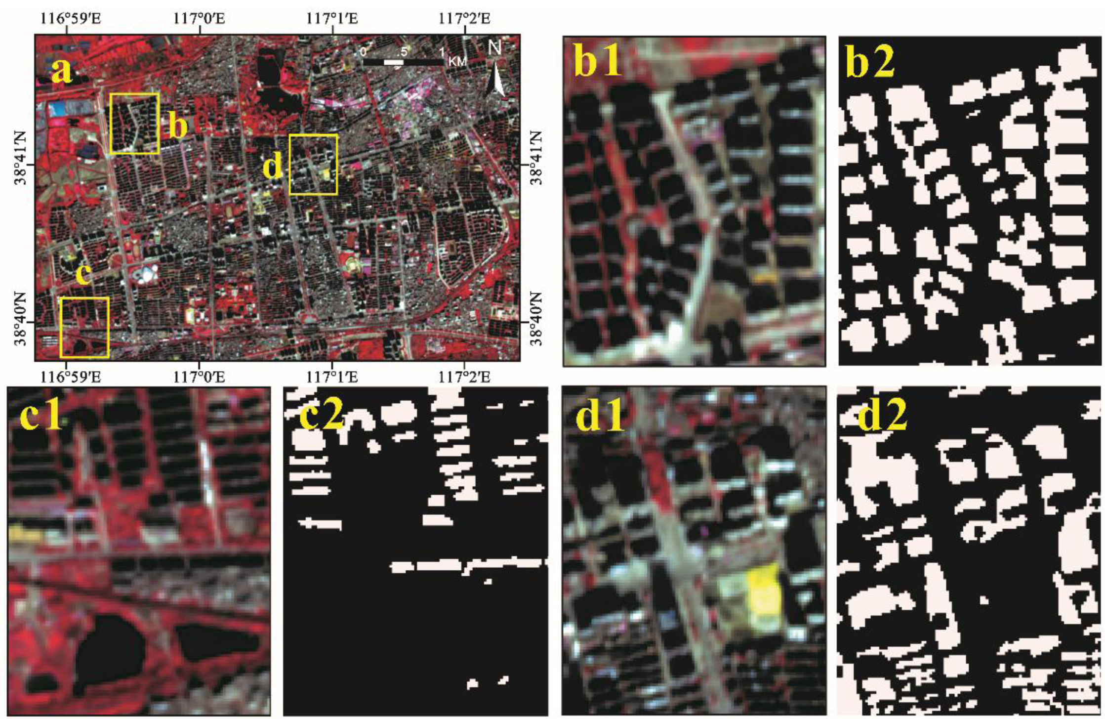
- The automated building shadow detection method in UWEM was used to address the misidentification caused by dark building shadows. Figure 8 shows the extracted shadow mask at the test site in Huainan where background has abundant dark shadows. Visual inspection of Figure 8 indicated good performance of the automated shadow detection method. For example, the method well detected shadows of different kinds of buildings (Figure 8b2). It can also well detect the shadows of tall buildings (Figure 8d2). What’s more, it performs well in the scenes where backgrounds have water bodies (Figure 8c2).

| Method | Aksu | Hanyang | Fuzhou | Huangpo | Huainan | ||||||||||
|---|---|---|---|---|---|---|---|---|---|---|---|---|---|---|---|
| Kappa | OE% | CE% | Kappa | OE% | CE% | Kappa | OE% | CE% | Kappa | OE% | CE% | Kappa | OE% | CE% | |
| HRWI | 0.91 | 15.58 | 1.97 | 0.97 | 3.04 | 1.90 | 0.78 | 30.37 | 11.33 | 0.96 | 5.07 | 2.21 | 0.83 | 28.94 | 0.60 |
| NDWI | 0.89 | 15.3 | 6.85 | 0.87 | 12.47 | 9.60 | 0.68 | 42.67 | 13.78 | 0.74 | 32.2 | 9.26 | 0.84 | 22.86 | 6.48 |
| UWEM | 0.96 | 4.53 | 3.99 | 0.98 | 1.42 | 2.22 | 0.90 | 6.81 | 12.53 | 0.96 | 5.07 | 2.21 | 0.96 | 4.27 | 3.24 |
| NDWIS | 0.89 | 15.3 | 6.85 | 0.88 | 11.75 | 8.94 | 0.68 | 42.67 | 13.78 | 0.74 | 32.2 | 9.26 | 0.88 | 20.89 | 1.59 |
6. Conclusions
Acknowledgments
Author Contributions
Conflicts of Interest
References
- Du, N.; Ottens, H.; Sliuzas, R. Spatial impact of urban expansion on surface water bodies—A case study of Wuhan, China. Landsc. Urban Plan. 2010, 94, 175–185. [Google Scholar] [CrossRef]
- Fletcher, T.D.; Andrieu, H.; Hamel, P. Understanding, management and modelling of urban hydrology and its consequences for receiving waters: A state of the art. Adv. Water Res. 2013, 51, 261–279. [Google Scholar] [CrossRef]
- Dewan, A.M.; Islam, M.M.; Kumamoto, T.; Nishigaki, M. Evaluating flood hazard for land-use planning in greater dhaka of bangladesh using remote sensing and GIS techniques. Water Res. Manag. 2006, 21, 1601–1612. [Google Scholar] [CrossRef]
- Lacaux, J.P.; Tourre, Y.M.; Vignolles, C.; Ndione, J.A.; Lafaye, M. Classification of ponds from high-spatial resolution remote sensing: Application to rift valley fever epidemics in Senegal. Remote Sens. Environ. 2007, 106, 66–74. [Google Scholar] [CrossRef]
- Viala, E. Water for food, water for life a comprehensive assessment of water management in agriculture. Irrig. Drain. Syst. 2008, 22, 127–129. [Google Scholar] [CrossRef]
- Eppink, F.V.; van den Bergh, J.C.; Rietveld, P. Modelling biodiversity and land use: Urban growth, agriculture and nature in a wetland area. Ecol. Econ. 2004, 51, 201–216. [Google Scholar] [CrossRef]
- Gessner, M.O.; Hinkelmann, R.; Nützmann, G.; Jekel, M.; Singer, G.; Lewandowski, J.; Nehls, T.; Barjenbruch, M. Urban water interfaces. J. Hydrol. 2014, 514, 226–232. [Google Scholar] [CrossRef]
- Pekel, J.F.; Vancutsem, C.; Bastin, L.; Clerici, M.; Vanbogaert, E.; Bartholomé, E.; Defourny, P. A near real-time water surface detection method based on HSV transformation of MODIS multi-spectral time series data. Remote Sens. Environ. 2014, 140, 704–716. [Google Scholar] [CrossRef]
- Goetz, S.; Gardiner, N.; Viers, J. Monitoring freshwater, estuarine and near-shore benthic ecosystems with multi-sensor remote sensing: An introduction to the special issue. Remote Sens. Environ. 2008, 112, 3993–3995. [Google Scholar] [CrossRef]
- Castañeda, C.; Herrero, J.; Auxiliadora Casterad, M. Landsat monitoring of playa-lakes in the spanish monegros desert. J. Arid Environ. 2005, 63, 497–516. [Google Scholar] [CrossRef]
- Feyisa, G.L.; Meilby, H.; Fensholt, R.; Proud, S.R. Automated water extraction index: A new technique for surface water mapping using landsat imagery. Remote Sens. Environ. 2014, 140, 23–35. [Google Scholar] [CrossRef]
- Frazier, P.S.; Page, K.J. Water body detection and delineation with Landsat TM data. Photogramm. Eng. Remote Sens. 2000, 66, 1461–1468. [Google Scholar]
- Haas, E.M.; Bartholomé, E.; Lambin, E.F.; Vanacker, V. Remotely sensed surface water extent as an indicator of short-term changes in ecohydrological processes in sub-saharan western Africa. Remote Sens. Environ. 2011, 115, 3436–3445. [Google Scholar] [CrossRef]
- Verpoorter, C.; Kutser, T.; Tranvik, L. Automated mapping of water bodies using Landsat multispectral data. Limnol. Oceanogr. Methods 2012, 10, 1037–1050. [Google Scholar] [CrossRef]
- Steele, M.K.; Heffernan, J.B. Morphological characteristics of urban water bodies: Mechanisms of change and implications for ecosystem function. Ecol. Appl. 2014, 24, 1070–1084. [Google Scholar] [CrossRef] [PubMed]
- Sawaya, K. Extending satellite remote sensing to local scales: Land and water resource monitoring using high-resolution imagery. Remote Sens. Environ. 2003, 88, 144–156. [Google Scholar] [CrossRef]
- Kingsford, R.; Wales, N.S. GIS Database for Wetlands of the Murray-Darling Basin; Murray-Darling Basin Commission: Sydney, Australia, 1997. [Google Scholar]
- Olmanson, L.G.; Bauer, M.E.; Brezonik, P.L. A 20-year Landsat water clarity census of Minnesota’s 10,000 lakes. Remote Sens. Environ. 2008, 112, 4086–4097. [Google Scholar] [CrossRef]
- Rogers, A.; Kearney, M. Reducing signature variability in unmixing coastal marsh thematic mapper scenes using spectral indices. Int. J. Remote Sens. 2004, 25, 2317–2335. [Google Scholar] [CrossRef]
- Jain, S.K.; Singh, R.; Jain, M.; Lohani, A. Delineation of flood-prone areas using remote sensing techniques. Water Res. Manag. 2005, 19, 333–347. [Google Scholar] [CrossRef]
- Sun, F.; Sun, W.; Chen, J.; Gong, P. Comparison and improvement of methods for identifying waterbodies in remotely sensed imagery. Int. J. Remote Sens. 2012, 33, 6854–6875. [Google Scholar] [CrossRef]
- McFeeters, S. The use of the Normalized Difference Water Index (NDWI) in the delineation of open water features. Int. J. Remote Sens. 1996, 17, 1425–1432. [Google Scholar] [CrossRef]
- Xu, H. Modification of Normalized Difference Water Index (NDWI) to enhance open water features in remotely sensed imagery. Int. J. Remote Sens. 2006, 27, 3025–3033. [Google Scholar] [CrossRef]
- Jiang, H.; Feng, M.; Zhu, Y.; Lu, N.; Huang, J.; Xiao, T. An automated method for extracting rivers and lakes from Landsat imagery. Remote Sens. 2014, 6, 5067–5089. [Google Scholar]
- Li, J.; Sheng, Y. An automated scheme for glacial lake dynamics mapping using Landsat imagery and digital elevation models: A case study in the Himalayas. Int. J. Remote Sens. 2012, 33, 5194–5213. [Google Scholar] [CrossRef]
- Fisher, A.; Danaher, T. A water index for spot 5 HRG satellite imagery, New South Wales, Australia, determined by linear discriminant analysis. Remote Sens. 2013, 5, 5907–5925. [Google Scholar] [CrossRef]
- Dare, P.M. Shadow analysis in high-resolution satellite imagery of urban areas. Photogramm. Eng. Remote Sens. 2005, 71, 169–177. [Google Scholar] [CrossRef]
- Li, Y.; Gong, P.; Sasagawa, T. Integrated shadow removal based on photogrammetry and image analysis. Int. J. Remote Sens. 2005, 26, 3911–3929. [Google Scholar] [CrossRef]
- Zhou, W.; Huang, G.; Troy, A.; Cadenasso, M.L. Object-based land cover classification of shaded areas in high spatial resolution imagery of urban areas: A comparison study. Remote Sens. Environ. 2009, 113, 1769–1777. [Google Scholar] [CrossRef]
- Tigges, J.; Lakes, T.; Hostert, P. Urban vegetation classification: Benefits of multitemporal rapideye satellite data. Remote Sens. Environ. 2013, 136, 66–75. [Google Scholar] [CrossRef]
- Brown, M.; Gunn, S.R.; Lewis, H.G. Support vector machines for optimal classification and spectral unmixing. Ecol. Model. 1999, 120, 167–179. [Google Scholar] [CrossRef]
- Fensholt, R.; Sandholt, I.; Stisen, S. Evaluating MODIS, MERIS, and VEGETATION vegetation indices using in situ measurements in a semiarid environment. IEEE Trans. Geosci. Remote Sens. 2006, 44, 1774–1786. [Google Scholar] [CrossRef]
- Mountrakis, G.; Im, J.; Ogole, C. Support vector machines in remote sensing: A review. ISPRS J. Photogramm. Remote Sens. 2011, 66, 247–259. [Google Scholar] [CrossRef]
- Foody, G.M.; Mathur, A. The use of small training sets containing mixed pixels for accurate hard image classification: Training on mixed spectral responses for classification by a SVM. Remote Sens. Environ. 2006, 103, 179–189. [Google Scholar] [CrossRef]
- van der Linden, S.; Waske, B.; Eiden, M.; Hostert, P.; Janz, A. Classifying segmented hyperspectral data from a heterogeneous urban environment using support vector machines. J. Appl. Remote Sens. 2007, 1. [Google Scholar] [CrossRef]
- Cao, X.; Chen, J.; Imura, H.; Higashi, O. A SVM-based method to extract urban areas from DMSP-OLS and SPOT VGT data. Remote Sens. Environ. 2009, 113, 2205–2209. [Google Scholar] [CrossRef]
- Kaufman, Y.J.; Remer, L. Detection of forests using mid-IR reflectance: An application for aerosol studies. IEEE Trans. Geosci. Remote Sens. 1994, 32, 672–683. [Google Scholar] [CrossRef]
- Adeline, K.R.M.; Chen, M.; Briottet, X.; Pang, S.K.; Paparoditis, N. Shadow detection in very high spatial resolution aerial images: A comparative study. ISPRS J. Photogramm. Remote Sens. 2013, 80, 21–38. [Google Scholar] [CrossRef]
- Luo, J.; Sheng, Y.; Shen, Z.; Li, J.; Gao, L. Automatic and high-precise extraction for water information from multispectral images with the step-by-step iterative transformation mechanism. J. Remote Sens. 2009, 13, 604–615. [Google Scholar]
- Kavzoglu, T.; Colkesen, I. A kernel functions analysis for support vector machines for land cover classification. Int. J. Appl. Earth Obs. Geoinf. 2009, 11, 352–359. [Google Scholar] [CrossRef]
- Ji, L.; Zhang, L.; Wylie, B. Analysis of dynamic thresholds for the normalized difference water index. Photogramm. Eng. Remote Sens. 2009, 75, 1307–1317. [Google Scholar] [CrossRef]
© 2015 by the authors; licensee MDPI, Basel, Switzerland. This article is an open access article distributed under the terms and conditions of the Creative Commons Attribution license (http://creativecommons.org/licenses/by/4.0/).
Share and Cite
Yao, F.; Wang, C.; Dong, D.; Luo, J.; Shen, Z.; Yang, K. High-Resolution Mapping of Urban Surface Water Using ZY-3 Multi-Spectral Imagery. Remote Sens. 2015, 7, 12336-12355. https://doi.org/10.3390/rs70912336
Yao F, Wang C, Dong D, Luo J, Shen Z, Yang K. High-Resolution Mapping of Urban Surface Water Using ZY-3 Multi-Spectral Imagery. Remote Sensing. 2015; 7(9):12336-12355. https://doi.org/10.3390/rs70912336
Chicago/Turabian StyleYao, Fangfang, Chao Wang, Di Dong, Jiancheng Luo, Zhanfeng Shen, and Kehan Yang. 2015. "High-Resolution Mapping of Urban Surface Water Using ZY-3 Multi-Spectral Imagery" Remote Sensing 7, no. 9: 12336-12355. https://doi.org/10.3390/rs70912336