
Comparative Analysis of MODIS Time-Series Classification Using Support Vector Machines and Methods Based upon Distance and Similarity Measures in the Brazilian Cerrado-Caatinga Boundary


 , and
, and
Abstract
:
1. Introduction
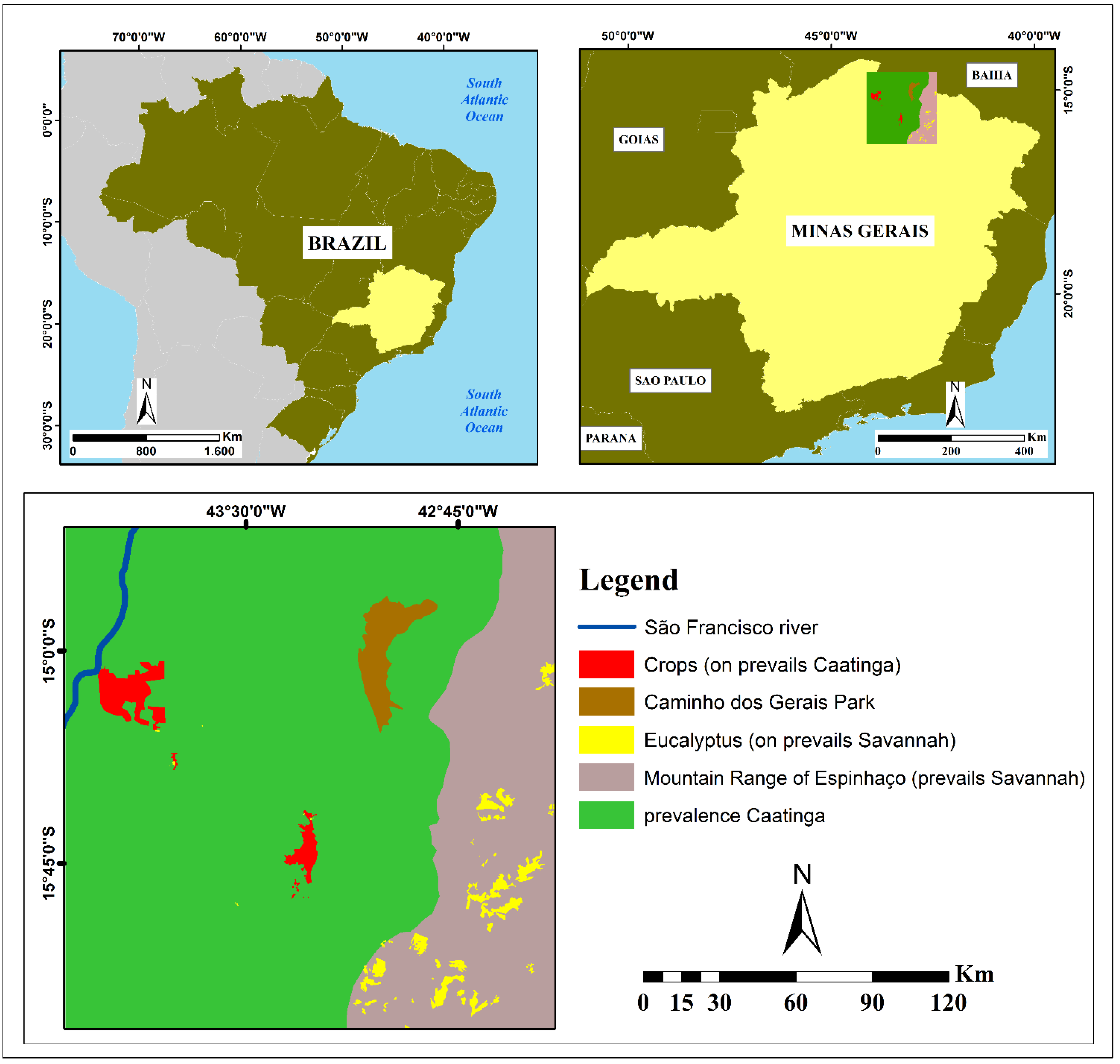
2. Study Area


| Climatic Data | Month | |||||||||||
|---|---|---|---|---|---|---|---|---|---|---|---|---|
| Jan. | Feb. | Mar. | Apr. | May | June | July | Aug. | Sept. | Oct. | Nov. | Dec. | |
| Rainfall (mm) | 175.6 | 96 | 93.3 | 33.1 | 8,0 | 5.4 | 15.1 | 31.4 | 31.2 | 54.2 | 117.8 | 150.7 |
| Average Temperature (°C) | 25.6 | 26 | 26.1 | 25.4 | 24.5 | 23.1 | 22.6 | 23.8 | 25.2 | 26.3 | 25.8 | 25.7 |
| Average Maximum Temperature (°C) | 30.8 | 31.5 | 31.5 | 31 | 30.4 | 29.1 | 28.8 | 30.3 | 31.6 | 32.5 | 31.2 | 30.8 |
| Average Minimum Temperature (°C) | 20.4 | 20.5 | 20.6 | 19.7 | 18.5 | 17 | 16.4 | 17.3 | 18.8 | 20.1 | 20.4 | 20.6 |
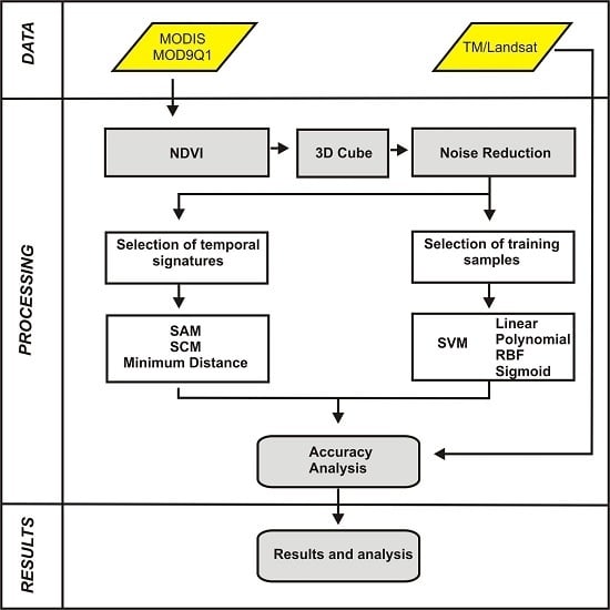
3. Methodology

3.1. MODIS/Terra Time-Series Dataset
3.2. Image Cube of NDVI-MODIS Time Series
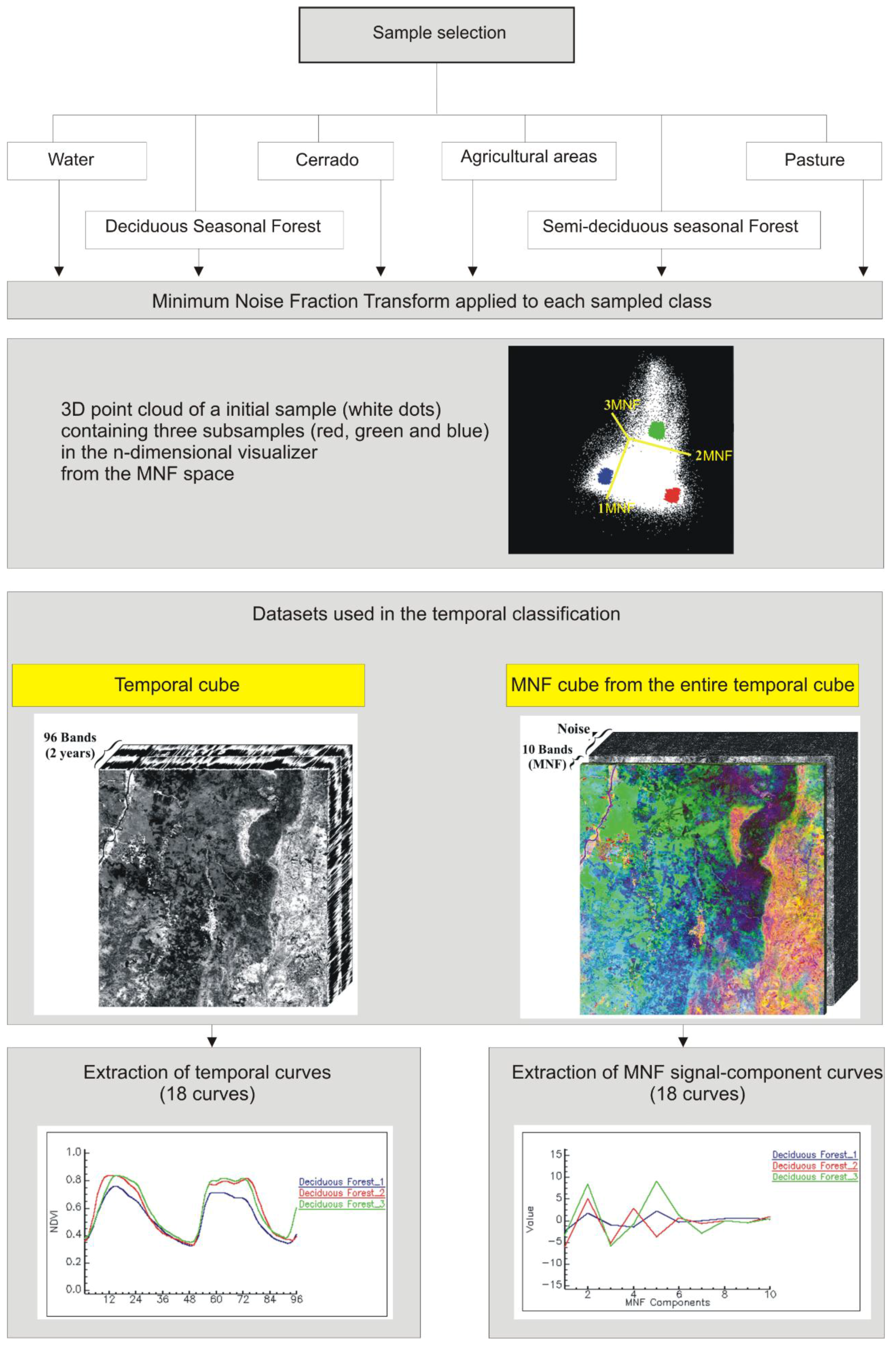
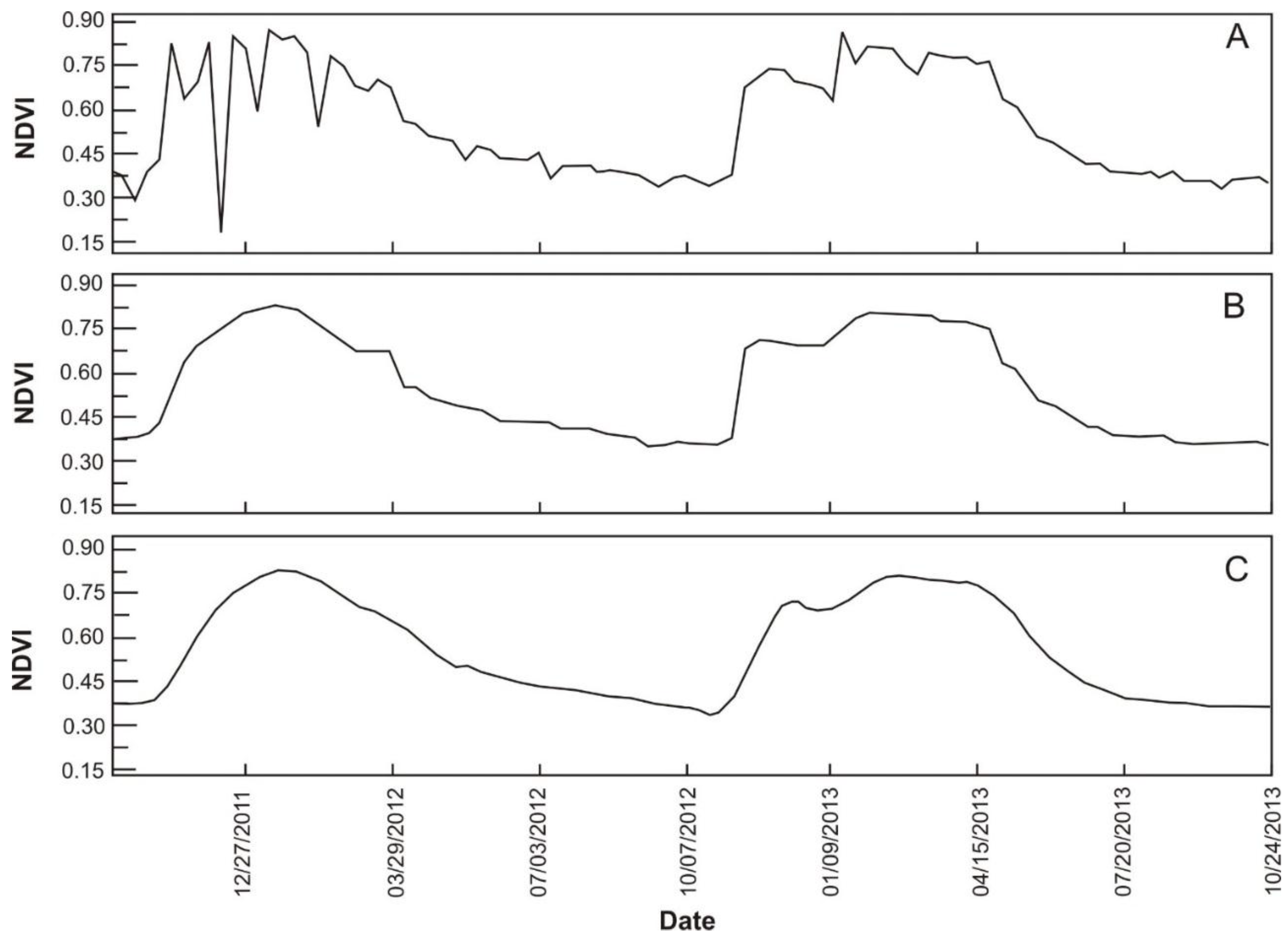
3.3. Image Denoising
3.4. Classification Using Distance and Similarity Measures
3.4.1. Reference Temporal-Signature Selection

| Sets | Specifications | Total Classes | Classes |
|---|---|---|---|
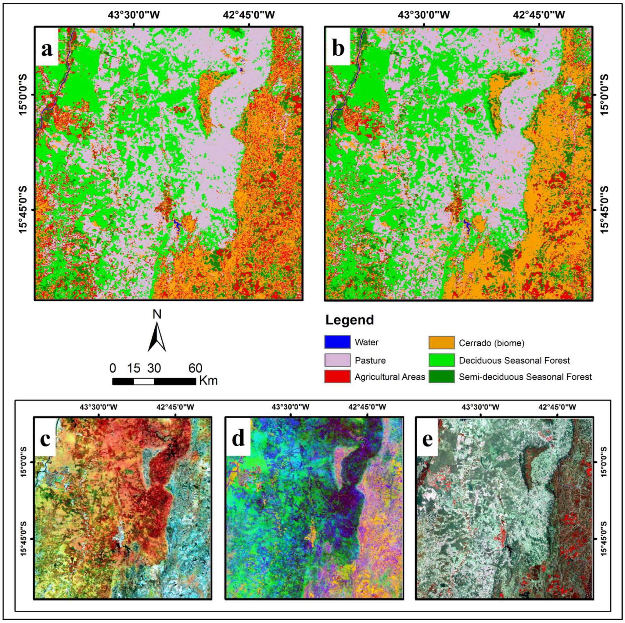
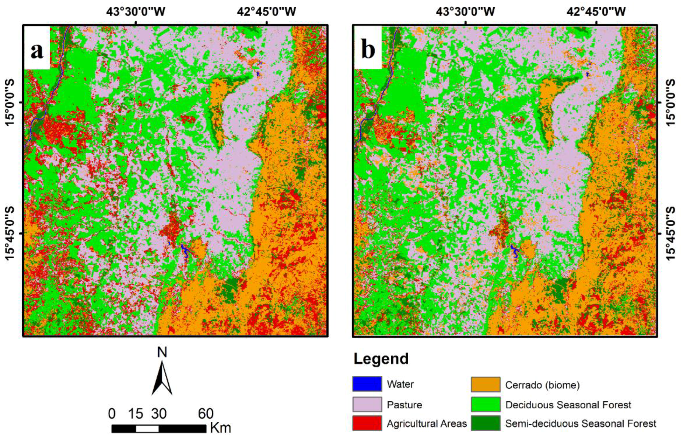
| 1 | Regional. Annual and perennial crops are not separated; vegetation subtypes of the Cerrado biome are not separated. | 6 | Water; Agricultural Areas 1, Pasture 1, Deciduous Seasonal Forest 2, Semi-deciduous Seasonal Forest 2, and Cerrado3. |
| 2 | Detailed. Annual and perennial crops are separated; woody and herbaceous formations of the Cerrado biome are separated. | 8 | Water, Annual Crops 1, Perennial Crops 1, Pasture 1, Deciduous Seasonal Forest 2, Semi-deciduous Seasonal Forest 2, Savanna Woodland (Cerrado stricto sensu) 3, and Grassland formations 3. |
3.4.2. Distance and Similarity Measures
3.5. Support Vector Machine
| Linear Kernel | Polynomial Kernel | RBF Kernel | Sigmoid Kernel |
|---|---|---|---|
3.6. Accuracy Analysis
4. Results
4.1. Noise Reduction
4.2. Classification using Distance and Similarity Measures
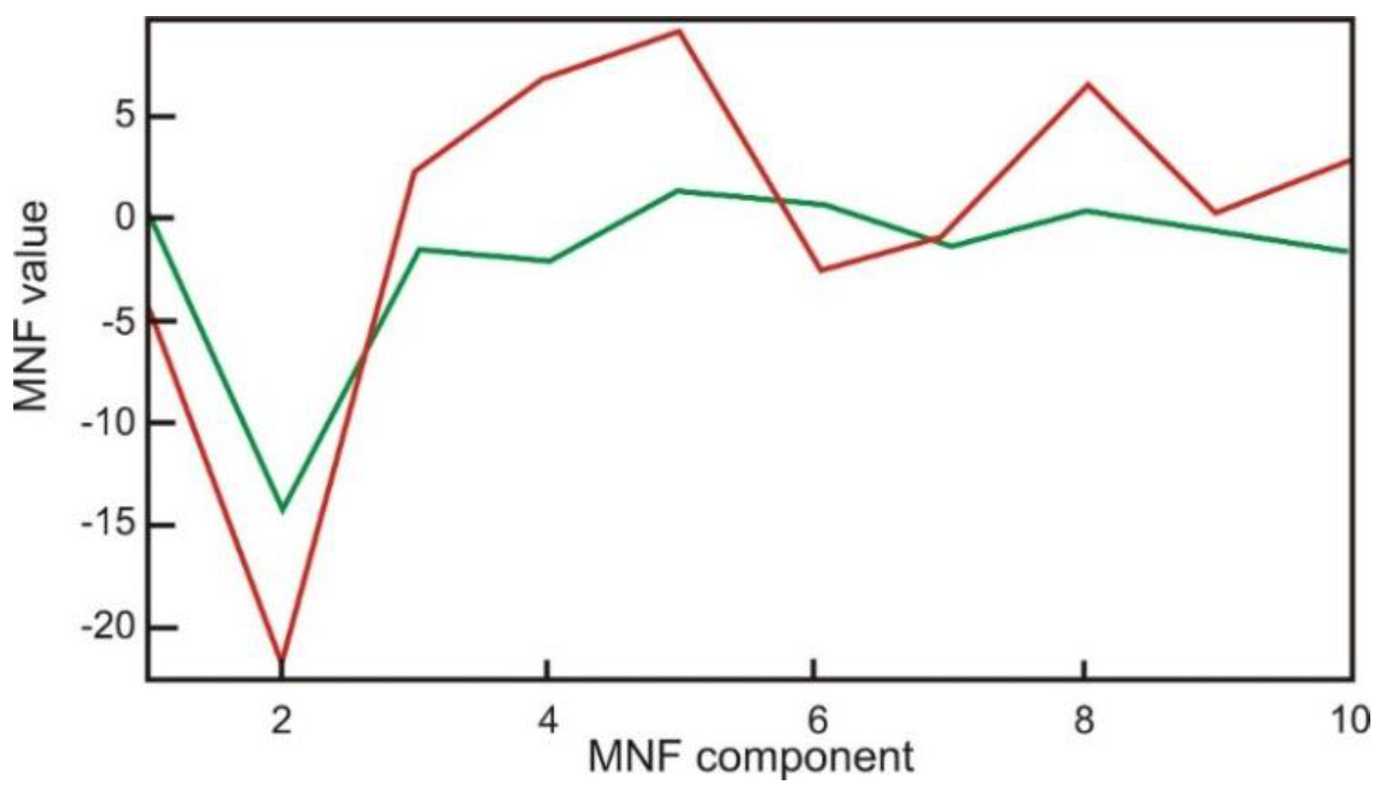
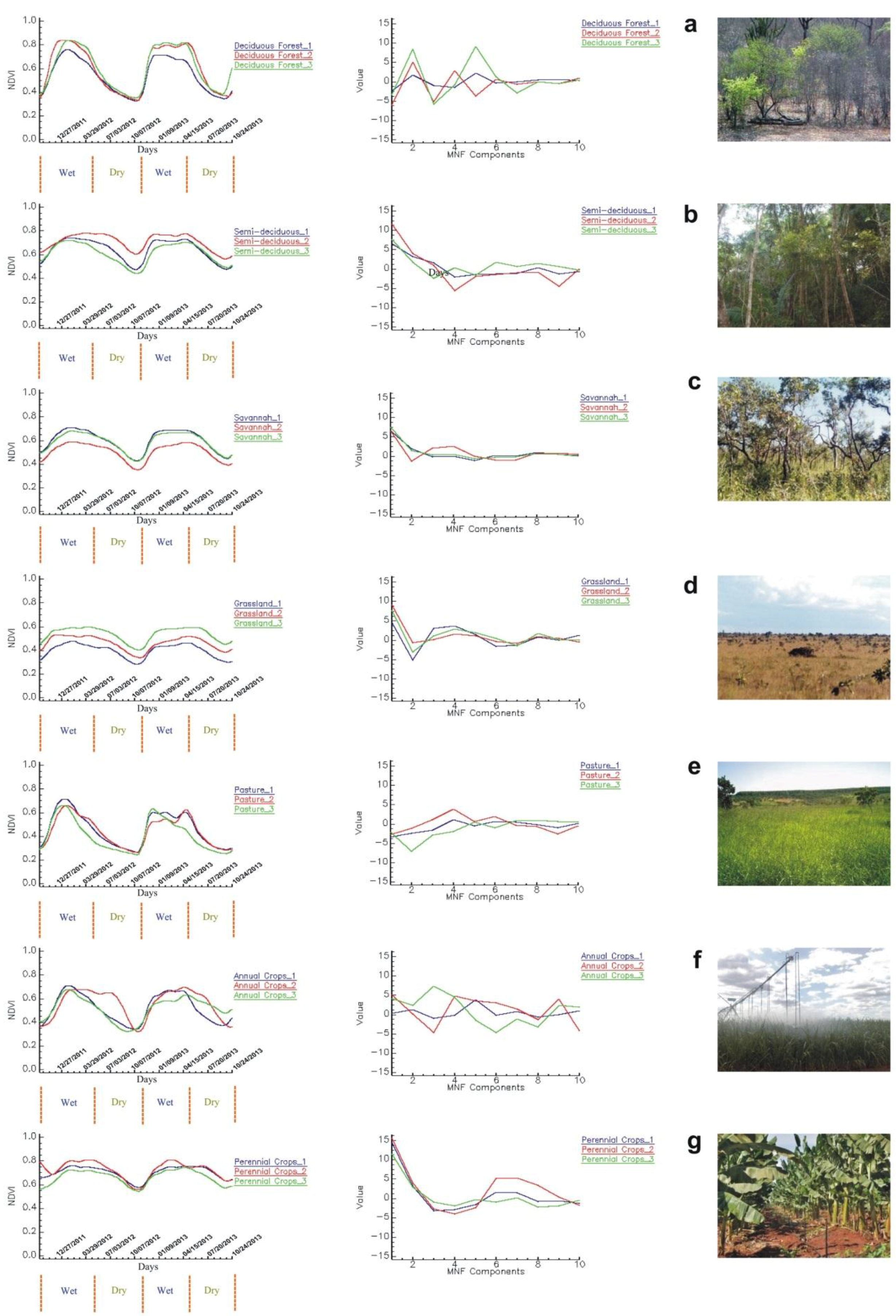
Reference Temporal Signatures

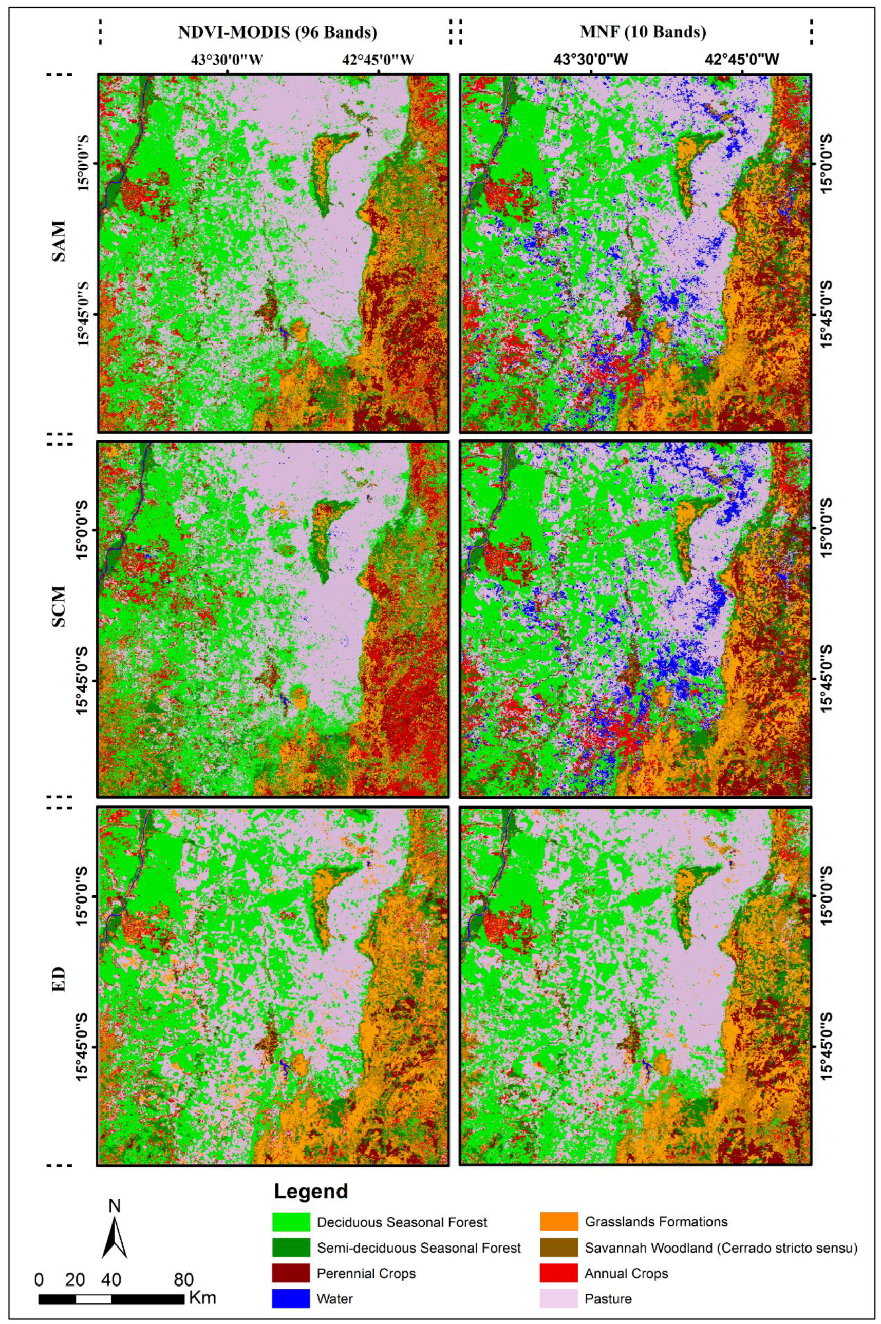
4.3. Classification of the MODIS-NDVI Time Series and MNF Signal Components
| One Temporal Signature per Class | |||||
|---|---|---|---|---|---|
| Method | Classes | Overall Accuracy | Kappa Coefficient | ||
| NDVI-MODIS | MNF Signal Components | NDVI-MODIS | MNF Signal Components | ||
| Euclidian Distance Measure | 6 | 73.50 | 72.43 | 0.67 | 0.66 |
| 8 | 67.25 | 64.75 | 0.62 | 0.59 | |
| Spectral Angle Mapper | 6 | 57.68 | 65.93 | 0.47 | 0.58 |
| 8 | 50.43 | 57.87 | 0.43 | 0.51 | |
| Spectral Correlation Mapper | 6 | 52.75 | 65.31 | 0.42 | 0.57 |
| 8 | 45.81 | 57.62 | 0.38 | 0.51 | |
| Three Temporal Signatures per Class | |||||
| Method | Classes | Overall Accuracy | Kappa Coefficient | ||
| NDVI-MODIS | Signal MNF | NDVI-MODIS | Signal MNF | ||
| Euclidian Distance Measure | 6 | 79.06 | 75.18 | 0.74 | 0.69 |
| 8 | 70.56 | 68.37 | 0.66 | 0.63 | |
| Spectral Angle Mapper | 6 | 60.81 | 68.43 | 0.51 | 0.61 |
| 8 | 54.68 | 61.37 | 0.48 | 0.55 | |
| Spectral Correlation Mapper | 6 | 55.25 | 66.18 | 0.45 | 0.58 |
| 8 | 45.18 | 60.06 | 0.37 | 0.54 | |

| MODIS-NDVI Data | |||||||||
|---|---|---|---|---|---|---|---|---|---|
| Class | Water | Annual Crops | Grassland Formations | Savanna Woodland | Deciduous | Pasture | Perennial Crops | Semi-Deciduous | Total |
| Water | 177 | 0 | 0 | 0 | 0 | 0 | 0 | 0 | 177 |
| Annual Crops | 1 | 110 | 11 | 9 | 3 | 7 | 2 | 1 | 144 |
| Grassland Formations | 17 | 23 | 90 | 64 | 1 | 11 | 2 | 2 | 210 |
| Savanna Woodland | 0 | 23 | 69 | 74 | 1 | 0 | 11 | 14 | 192 |
| Deciduous | 0 | 26 | 8 | 10 | 181 | 3 | 0 | 1 | 229 |
| Pasture | 5 | 13 | 6 | 1 | 12 | 179 | 0 | 0 | 216 |
| Perennial Crops | 0 | 1 | 5 | 8 | 0 | 0 | 158 | 22 | 194 |
| Semi-deciduous | 0 | 4 | 11 | 34 | 2 | 0 | 27 | 160 | 238 |
| Total | 200 | 200 | 200 | 200 | 200 | 200 | 200 | 200 | 1600 |
| MNF-Signal Components | |||||||||
| Class | Water | Annual Crops | Grassland Formations | Savanna Woodland | Deciduous | Pasture | Perennial Crops | Semi-Deciduous | Total |
| Water | 171 | 0 | 0 | 0 | 0 | 0 | 0 | 0 | 171 |
| Annual Crops | 1 | 112 | 10 | 10 | 2 | 0 | 0 | 4 | 139 |
| Grassland Formations | 17 | 11 | 105 | 60 | 1 | 4 | 0 | 1 | 199 |
| Savanna Woodland | 2 | 12 | 40 | 60 | 1 | 1 | 6 | 29 | 151 |
| Deciduous | 0 | 20 | 5 | 11 | 155 | 8 | 0 | 4 | 203 |
| Pasture | 9 | 25 | 8 | 5 | 41 | 187 | 0 | 0 | 275 |
| Perennial Crops | 0 | 9 | 11 | 15 | 0 | 0 | 165 | 23 | 223 |
| Semi-deciduous | 0 | 11 | 21 | 39 | 0 | 0 | 29 | 139 | 239 |
| Total | 200 | 200 | 200 | 200 | 200 | 200 | 200 | 200 | 1600 |

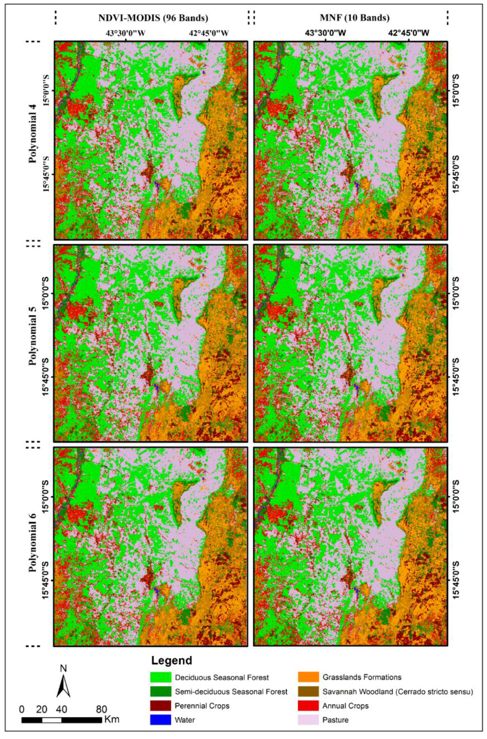
4.4. Classification Using SVMs
| Method | Classes | Overall Accuracy | Kappa Coefficient | ||
|---|---|---|---|---|---|
| NDVI-MODIS | MNF Signal Components | NDVI-MODIS | MNF Signal Components | ||
| Linear | 6 | 78.81 | 79.00 | 0.739 | 0.742 |
| 8 | 72.43 | 73.00 | 0.685 | 0.691 | |
| Polynomial 2 | 6 | 80.18 | 78.93 | 0.756 | 0.741 |
| 8 | 73.87 | 72.93 | 0.701 | 0.690 | |
| Polynomial 3 | 6 | 80.12 | 79.37 | 0.755 | 0.746 |
| 8 | 73.87 | 73.18 | 0.701 | 0.693 | |
| Polynomial 4 | 6 | 80.75 | 79.81 | 0.763 | 0.752 |
| 8 | 74.37 | 73.75 | 0.707 | 0.700 | |
| Polynomial 5 | 6 | 80.62 | 80.06 | 0.762 | 0.755 |
| 8 | 74.43 | 74.12 | 0.707 | 0.704 | |
| Polynomial 6 | 6 | 80.12 | 80.56 | 0.755 | 0.761 |
| 8 | 74.12 | 74.56 | 0.704 | 0.709 | |
| RBF | 6 | 80.43 | 80.06 | 0.759 | 0.755 |
| 8 | 74.25 | 73.93 | 0.705 | 0.702 | |
| Sigmoid | 6 | 65.68 | 78.18 | 0.574 | 0.732 |
| 8 | 58.12 | 72.37 | 0.521 | 0.684 | |


5. Discussion
6. Conclusions
Acknowledgments
Author Contributions
Conflicts of Interest
References
- Werneck, F.P. The diversification of Eastern South American open vegetation biomes: Historical biogeography and perspectives. Quat. Sci. Rev. 2011, 30, 1630–1648. [Google Scholar] [CrossRef]
- Pinheiro, M.H.O.; MONTEIRO, R. Contribution to the discussions on the origin of the Cerrado biome: Brazilian savanna. Braz. J. Biol. 2010, 70, 95–102. [Google Scholar] [CrossRef] [PubMed]
- Pennigton, R.T.; Lavin, M.; Oliveira-Filho, A. Woody plant diversity, evolution, and ecology in the tropics: Perspectives from seasonally dry tropical forests. Annu. Rev. Evol. Sust. 2009, 40, 437–457. [Google Scholar] [CrossRef]
- Hoekstra, J.M.; Boucher, T.M.; Ricketts, T.H.; Roberts, C. Confronting a biome crisis: Global disparities of habitat loss and protection. Ecol. Lett. 2005, 8, 23–29. [Google Scholar] [CrossRef]
- Portillo-Quintero, C.A.; Sánchez-Azofeifa, G.A. Extent and conservation of tropical dry forests in the Americas. Biol. Cons. 2010, 143, 144–155. [Google Scholar] [CrossRef]
- Boori, M.S.; Amaro, V.E. Land use change detection for environmental management: Using multi-temporal, satellite data in the Apodi Vallery of northeastern Brazil. Appl. GIS 2010, 6, 1–15. [Google Scholar]
- Ministério do Meio Ambiente (MMA); Instituto Brasileiro do Meio Ambiente e dos Recursos Naturais Renováveis (IBAMA). Monitoramento do Bioma Caatinga 2008–2009. In Monitoramento dos Desmatamentos nos Biomas Brasileiros por Satélite; MMA: Brasília, Brazil, 2011; pp. 1–46. [Google Scholar]
- Sano, E.E.; Rosa, R.; Brito, J.L.S.; Ferreira, L.G. Land cover mapping of the tropical savanna region in Brazil. Environ. Monit. Assess. 2010, 166, 113–124. [Google Scholar] [CrossRef] [PubMed]
- Furley, P.A.; Metcalfe, S.E. Dynamic changes in savanna and seasonally dry vegetation through time. Prog. Phys. Geog. 2007, 31, 633–642. [Google Scholar] [CrossRef]
- Werneck, F.P.; Costa, G.C.; Colli, G.R.; Prado, D.E.; Sites, J.W., Jr. Revisiting the historical distribution of seasonally dry tropical forests: New insights based on palaeodistribution modelling and palynological evidence. Global Ecol. Biogeogr. 2011, 20, 272–288. [Google Scholar] [CrossRef]
- Justice, C.O.; Townshend, J.R.G.; Vermote, E.F.; Masuoka, E.; Wolfe, R.E.; Saleous, N.; Roy, D.P.; Morisette, J.T. An overview of MODIS land data processing and product status. Remote Sens. Environ. 2002, 83, 3–15. [Google Scholar] [CrossRef]
- Hammer, D.; Kraft, R.; Wheeler, D. Alerts of forest disturbance from MODIS imagery. Int. J. Appl. Earth Obs. Geoinf. 2014, 33, 1–9. [Google Scholar] [CrossRef]
- Van Leeuwen, W.J.; Davison, J.E.; Casady, G.M.; Marsh, S.E. Phenological characterization of desert sky Island vegetation communities with remotely sensed and climate time series data. Remote Sens. 2010, 2, 388–415. [Google Scholar] [CrossRef]
- Zhao, X.; Xu, P.; Zhou, T.; Li, Q.; Wu, D. Distribution and variation of forests in China from 2001 to 2011: A study based on remotely sensed data. Remote Sens. Environ. 2013, 4, 632–649. [Google Scholar] [CrossRef]
- Bernardes, T.; Moreira, M.A.; Adami, M.; Giarolla, A.; Rudorff, B.F.T. Monitoring biennial bearing effect on coffee yield using MODIS remote sensing imagery. Remote Sens. 2012, 4, 2492–2509. [Google Scholar] [CrossRef]
- Couto Júnior, A.F.; de Carvalho Júnior, O.A.; Martins, E.S.; Vasconcelos, V. Characterization of the agriculture occupation in the Cerrado biome using MODIS time-series. Rev. Bras. Geofis. 2013, 31, 393–402. [Google Scholar]
- Galford, G.; Mustard, J.F.; Melillo, J.; Gendrin, A.; Cerri, C.C.; Cerri, C.E.P. Wavelet analysis of MODIS time series to detect expansion and intensification of row-crop agriculture in Brazil. Remote Sens. Environ. 2008, 112, 576–587. [Google Scholar] [CrossRef]
- Pan, Y.; Li, L.; Zhang, J.; Liang, S.; Zhu, X.; Sulla-Menashe, D. Winter wheat area estimation from MODIS-EVI time series data using the crop proportion phenology index. Remote Sens. Environ. 2012, 119, 232–242. [Google Scholar] [CrossRef]
- Sakamoto, T.; Yokozawa, M.; Toritani, H.; Shibayama, M.; Ishitsuka, N.; Ohno, H. A crop phenology detection method using time-series MODIS data. Remote Sens. Environ. 2005, 96, 366–374. [Google Scholar] [CrossRef]
- Ferreira, L.G.; Fernandez, L.E.; Sano, E.E.; Field, C.; Sousa, S.B.; Arantes, A.E.; Araújo, F.M. Biophysical properties of cultivated pastures in the Brazilian savanna biome: An analysis in the spatial-temporal domains based on ground and satellite data. Remote Sens. 2013, 5, 307–326. [Google Scholar] [CrossRef]
- Le Maire, G.; Marsden, C.; Nouvellon, Y.; Stape, J.L.; Ponzoni, F.J. Calibration of a species-specific spectral vegetation index for leaf area index (LAI) monitoring: Example with MODIS reflectance time-series on eucalyptus plantations. Remote Sens. 2012, 4, 3766–3780. [Google Scholar] [CrossRef] [Green Version]
- Sánchez-Azofeifa, G.A.; Quesada, M.; Rodríguez, J.P.; Nassar, J.M.; Stoner, K.E.; Castillo, A.; Garvin, T.; Zent, E.L.; Calvo-Alvarado, J.C.; Kalacska, M.E.R.; et al. Research priorities for neotropical dry forests. Biotropica 2005, 37, 477–485. [Google Scholar]
- Hüttich, C.; Gessner, U.; Herold, M.; Strohbach, B.J.; Schimidt, M.; Keil, M.; Dech, S. On the suitability of MODIS time series metrics to map vegetation types in dry savana ecosystems: A case study in the Kalahari of NE Namibia. Remote Sens. 2009, 1, 620–643. [Google Scholar] [CrossRef]
- Baldi, G.; Houspanossian, J.; Murray, F.; Rosales, A.A.; Rueda, C.V.; Jobbágy, E.G. Cultivating the dry forests of South America: Diversity of land users and imprints on ecosystem functioning. J. Arid. Environ. 2014. [Google Scholar] [CrossRef]
- Portillo-Quintero, C.A.; Sánchez-Azofeifa, G.A.; Espírito-Santo, M.M. Monitoring deforestation with MODIS active fires in neotropical dry forests: An analysis of local-scale assessments in Mexico, Brazil and Bolivia. J. Arid Environ. 2013, 97, 150–159. [Google Scholar] [CrossRef]
- Madeira, B.G.; Espírito-Santo, M.M.; D’Ângelo Neto, S.; Nunes, Y.R.F.; Sánchez-Azofeifa, G.A.; Fernandes, G.W.; Quesada, M. Changes in tree and liana communities along a sucessional gradiente in a tropical dry forest in South-Eastern Brazil. Plant. Ecol. 2009, 201, 291–304. [Google Scholar] [CrossRef]
- Instituto Nacional de Meteorologia (INMET). Banco de Dados Meteorológicos para Ensino e Pesquisa (BDMEP). Available online: http://www.inmet.gov.br (accessed on 21 April 2015).
- Saadi, A.; Magalhães Júnior, A.P. A geomorfologia do Planalto do Espinhaço setentrional avaliada para a implantação de barragem: A UHE de Irapé-MG. Geonomos 1997, 5, 9–14. [Google Scholar]
- De Carvalho, L.M.T.; Scolforo, J.R. Inventário Florestal de Minas Gerais: Monitoramento da Flora Nativa 2005–2007, 1st ed.; Lavras: Universidade Federal de Lavras, Brazil, 2008; p. 357. [Google Scholar]
- Dutra, V.F.; Garcia, F.C.P. Three New Species of Mimosa (Leguminosae) from Minas Gerais, Brazil. Syst. Botany 2013, 38, 398–405. [Google Scholar] [CrossRef]
- Alves, R.J.V.; Kolbek, J. Can campo rupestre vegetation be floristically delimited based on vascular plant genera? Plant Ecol. 2010, 207, 67–79. [Google Scholar] [CrossRef]
- Echternacht, L.; Trovó, M.; Oliveira, C.T.; Pirani, J.R. Areas of endemismo in the Espinhaço Range in Minas Gerais, Brazil. Flora 2011, 206, 782–791. [Google Scholar] [CrossRef]
- Espírito-Santo, M.M.; Sevilha, A.C.; Anaya, F.C.; Barbosa, R.; Fernandes, G.W.; Sánchez-Azofeifa, G.A.; Scariot, A.; de Noronha, S.E.; Sampaio, C.A. Sustainability of tropical dry forests: Two case studies in southeastern and central Brazil. Forest Ecol. Manag. 2009, 258, 922–930. [Google Scholar] [CrossRef]
- Zappi, D. Fitofisionomia da Caatinga associada à Cadeia do Espinhaço. Megadiversidade 2008, 4, 34–38. [Google Scholar]
- Instituto Brasileiro de Geografia e Estatística (IBGE). Sistema IBGE de Recuperação Eletrônica (SIDRA). Available online: http://www.sidra.ibge.gov.br (accessed on 29 August 2014).
- Domingues, S.A.; Karez, C.S.; Biondini, I.V.F.; Andrade, M.A.; Fernandes, G.W. Economic environmental management tolls in the Serra do Espinhaço biosphere reserve. J. Sust. Dev. 2012, 5, 180–191. [Google Scholar]
- Dos Santos, R.M.; Vieira, F.A.; Fagundes, M.; Nunes, Y.R.F.; Gusmão, F. Floristic richness and similarity of eight forest remnants in the north of Minas Gerais state, Brazil. Rev. Árvore 2007, 31, 135–144. [Google Scholar]
- Vermote, E.F.; Kotchenova, S.Y. MOD09 (Surface Reflectance) User’s Guide; MODIS Land Surface Reflectance Science Computing Facility: College Park, MD, USA, 2008. [Google Scholar]
- Huete, A.; Didan, K.; Miura, T.; Rodriguez, E.P.; Gao, X.; Ferreira, L.G. Overview of the radiometric and biophysical performance of the MODIS vegetation indices. Remote Sens. Environ. 2002, 83, 195–213. [Google Scholar] [CrossRef]
- Guindin-Garcia, N.; Gitelson, A.A.; Arkebauer, T.J.; Shanahan, J.; Weiss, A. An evaluation of MODIS 8- and 16-day composite products for monitoring maize leaf are index. Agric. For. Meteorol. 2012, 161, 15–25. [Google Scholar] [CrossRef]
- Lisenberg, V.; Ponzoni, F.J.; Galvão, L.S. Analysis of the seasonal dynamics and spectral separability of some savanna physiognomies with vegetation indices derived from MODIS/TERRA and AQUA. Rev. Árvore 2007, 31, 295–305. [Google Scholar]
- Rouse, J.W.; Haas, R.H.; Schell, J.A.; Deering, D.W. Monitoring vegetation systems in the Great Plains with ERTS. In Proceedings of the Third Earth Resources Technology Satellite-1 Symposium, Greenbelt, MD, USA, 10–15 December 1973; pp. 301–317.
- De Carvalho Júnior, O.A.; Hermuche, P.M.; Guimarães, R.F. Identificação regional da floresta decidual na bacia do rio Paranã a partir da análise multitemporal de imagens MODIS. Rev. Bras. Geofis. 2006, 24, 319–332. [Google Scholar] [CrossRef]
- De Carvalho Júnior, O.A.; Sampaio, C.S.; da Silva, N.C.; Couto Júnior, A.F.; Gomes, R.A.T.; de Carvalho, A.P.F.; Shimabukuro, Y.E. Classificação de padrões de savana usando assinaturas temporais NDVI do sensor MODIS no parque nacional Chapada dos Veadeiros. Rev. Bras. Geofis. 2008, 26, 505–517. [Google Scholar] [CrossRef]
- Savitzky, A.; Golay, M.J.E. Smoothinbg and differentiation of data by simplified least squares procedures. Anal. Chem. 1964, 36, 1627–1639. [Google Scholar] [CrossRef]
- Ataman, E.; Aatre, V.K.; Wong, K.M. Some statistical properties of median filters. IEEE T. Acoust. Speech 1981, 29, 1073–1075. [Google Scholar] [CrossRef]
- De Carvalho Júnior, O.A.; da Silva, N.C.; de Carvalho, A.P.F.; Couto Júnior, A.F.; Silva, R.S.; Shimabukuro, Y.E.; Guimarães, R.F.; Gomes, R.A.T. Combining noise-adjusted principal components transform and median filter techniques for denoising MODIS temporal signatures. Rev. Bras. Geofis. 2012, 30, 147–157. [Google Scholar]
- Schefer, R.W. What is a Savitzky-Golay filter? IEEE Signal Process. Mag. 2011, 28, 111–117. [Google Scholar] [CrossRef]
- Chen, J.; Jönsson, P.; Tamura, M.; Gu, Z.; Matsushita, B.; Eklundh, L. A simple method for reconstructing a high-quality NDVI time-series data set based on the Savitzky-Golay filter. Remote Sens. Environ. 2004, 91, 332–334. [Google Scholar] [CrossRef]
- Li, L.; Friedl, M.A.; Xin, Q.; Gray, J.; Pan, Y.; Frolking, S. Mapping crop cycles in China using MODIS-EVI time series. Remote Sens. 2014, 6, 2473–2493. [Google Scholar] [CrossRef]
- Vrieling, A.; de Leeuw, J.; Said, M.Y. Length of growing period over Africa: Variability and trends from 30 years of NDVI time series. Remote Sens. 2013, 5, 982–1000. [Google Scholar] [CrossRef]
- Geng, L.; Ma, M.; Wang, X.; Yu, W.; Jia, S.; Wang, H. Comparison of eight techniques for reconstructing multi-satellite sensor time-series NDVI data sets in the Heihe River Basin, China. Remote Sens. 2014, 6, 2024–2049. [Google Scholar] [CrossRef]
- Atkinson, P.M.; Jeganathan, C.; Dash, J.; Atzberger, C. Inter-comparison of four models for smoothing satellite sensor time-series data to estimate vegetation phenology. Remote Sens. Environ. 2012, 123, 400–417. [Google Scholar] [CrossRef]
- De Beurs, K.M.; Henebry, G.M. Spatio-temporal statistical methods for modelling land surface phenology. In Phenological research, Methods for Environmental and Climate Change Analysis, 1st ed.; Hudson, I.L., Keatley, M.R., Eds.; Springer: Dordrecht, Netherlands, 2010; pp. 177–208. [Google Scholar]
- Hird, J.N.; McDermid, G.J. Noise reduction of NDVI time series: An empirical comparison of selected techniques. Remote Sens. Environ. 2009, 113, 248–258. [Google Scholar] [CrossRef]
- Adams, J.B.; Gillespie, A.R. Remote Sensing of Landscapes with Spectral Images: A Physical Modeling Approach; Cambridge University Press: New York, NY, USA, 2006; p. 362. [Google Scholar]
- Kruse, F.; Boardman, J.W.; Huntington, J.F. Comparison of airborne hyperspectral data and EO-1 Hyperion for mineral mapping. IEEE Trans. Geosci. Remote Sens. 2003, 41, 1388–1400. [Google Scholar] [CrossRef]
- Boardman, J. W. Automating spectral unmixing of AVIRIS data using convex geometry concepts. In Summaries of the Fourth Annual JPL Airborne Geosciences Workshop; Robert, O.G., Ed.; Jet Propulsion Laboratory Publication: Pasadena, CA, USA, 25–29 October 1993; pp. 11–14. [Google Scholar]
- Craig, M. Minimum-volume transforms for remotely sensed data. IEEE Trans. Geosci. Remote Sens. 1994, 32, 542–552. [Google Scholar] [CrossRef]
- Boardman, J.W.; Kruse, F.A. Analysis of imaging spectrometer data using n-dimensional geometry and a mixture-tuned matched filtering approach. IEEE Trans. Geosci. Remote Sens. 2011, 49, 4138–4152. [Google Scholar] [CrossRef]
- Green, A.A.; Berman, M.; Switzer, P.; Craig, M.D. A transformation for ordering multispectral data in terms of images quality with implications for noise removal. IEEE Trans. Geosci. Remote Sens. 1988, 26, 65–74. [Google Scholar] [CrossRef]
- Instituto Estadual de Florestas de Minas Gerais (IEF). Mapeamento da Cobertura Vegetal de Minas Gerais. Available online: http://www.inventarioflorestal.mg.gov.br (accessed on 16 July 2014).
- Dickson, B.L.; Taylor, G.F. Maximum noise fraction method reveals detail in aerial gamma-ray surveys. Explor. Geophys. 2000, 31, 73–77. [Google Scholar] [CrossRef]
- De Carvalho Júnior, O.A.; Maciel, L.M.M.; de Carvalho, A.P.F.; Guimarães, R.F.; Silva, C.R.; Gomes, R.A.T.; Silva, N.C. Probability density components analysis: A new approach to treatment and classification of SAR images. Remote Sens. 2014, 6, 2989–3019. [Google Scholar]
- Bateson, C.A.; Curtiss, B. A method for manual endmember selection and spectral unmixing. Remote Sens. Environ. 1996, 55, 229–243. [Google Scholar]
- Bateson, C.; Asner, G.P.; Wessman, C. Endmember bundles: A new approach to incorporating endmember variability into spectral mixture analysis. IEEE Trans. Geosci. Remote Sens. 2000, 38, 1083–1094. [Google Scholar] [CrossRef]
- Chan, T.H.; Chi, C.Y.; Huang, Y.M.; Ma, W.K. A convex analysis-based minimum-volume enclosing simplex algorithm for hyperspectral unmixing. IEEE Trans. Signal Process. 2009, 57, 4418–4432. [Google Scholar] [CrossRef]
- Chang, C.I.; Wu, C.C.; Liu, W.M.; Ouyang, Y.C. A new growing method for simplex-based endmember extraction algorithm. IEEE Trans. Geosci. Remote Sens. 2006, 44, 2804–2819. [Google Scholar] [CrossRef]
- Winter, M.E. N-FINDER: An algorithm for fast autonomous spectral endmember determination in hyperspectral data. In Proceedings of the SPIE 3753, Imaging Spectrometry, Denver, CO, USA, October 1999; pp. 266–277. [CrossRef]
- Kruse, F.A.; Lefkoff, A.B.; Boardman, J.W.; Heidebrecht, K.B.; Shapiro, A.T.; Barloon, P.J.; Goetz, A.F.H. The spectral imageprocessing system (SIPS)—Interactive visualization and analysis of imaging spectrometer data. Remote Sens. Environ. 1993, 44, 145–163. [Google Scholar] [CrossRef]
- De Carvalho Júnior, O.A.; Meneses, P.R. Spectral Correlation Mapper (SCM): An improving on the Spectral Angle Mapper (SAM). In Proceedings of Ninth Annual JPL Airborne Earth Science Workshop, Pasadena, CA, USA, 23–25 February 2000; pp. 65–74.
- De Carvalho Júnior, O.A.; Guimarães, R.F.; Gillespie, A.R.; Silva, N.C.; Gomes, R.A.T. A new approach to change vector analysis using distance and similarity measures. Remote Sens. 2011, 3, 2473–2493. [Google Scholar] [CrossRef]
- De Carvalho Júnior, O.A.; Guimarães, R.F.; Silva, N.C.; Gillespie, A.R.; Gomes, R.A.T.; Silva, C.R.; de Carvalho, A.P.F. Radiometric normalization of temporal images combining automatic detection of pseudo-invariant features from the distance and similarity spectral measures, density scatterplot analysis, and robust regression. Remote Sens. 2013, 5, 2763–2794. [Google Scholar]
- Vapnik, V. Estimation of Dependences Based on Empirical Data; Springer Verlag: New York, NY, USA, 1982. [Google Scholar]
- Kecman, V. Support vector machines—An introduction. In Support Vector Machines: Theory and Applications, 1st ed.; Wang, L., Ed.; Springer Science & Business Media: Heidelberg, Germany, 2005; pp. 1–47. [Google Scholar]
- Shmilovici, A. Support vector machines. In Data Mining and Knowledge Discovery Handbook, 1st ed.; Maimon, O., Rokach, L., Eds.; Springer: USA, 2005; pp. 257–276. [Google Scholar]
- Schölkopf, B.; Smola, A.J. Learning with Kernels: Support Vector Machines, Regularization, Optimization, and Beyond; The MIT Press: Cambridge, MA, USA, 2002. [Google Scholar]
- Lu, J.; Plataniotis, K.N.; Venetsanopoulos, A.N. Kernel Discriminant Learning with Application to Face Recognition. In Support Vector Machines: Theory and Applications, 1st ed.; Wang, L., Ed.; Springer Science & Business Media: Heidelberg, Germany, 2005; pp. 275–296. [Google Scholar]
- Mountrakis, G.; Im, J.; Ogole, C. Support vector machines in remote sensing: A review. ISPRS J. Photogramm. Remote Sens. 2011, 66, 247–259. [Google Scholar] [CrossRef]
- Carrão, H.; Gonçalves, P.; Caetano, M. Contribution of multispectral and multitemporal information from MODIS images to land cover classification. Remote Sens. Environ. 2008, 112, 986–997. [Google Scholar] [CrossRef]
- Vuolo, F.; Atzberger, C. Exploiting the classification performance of support vector machines with multi-temporal Moderate-Resolution Imaging Spectroradiometer (MODIS) data in areas of agreement and disagreement of existing land cover products. Remote Sens. 2012, 4, 3143–3167. [Google Scholar] [CrossRef]
- Chang, C.C.; Lin, C.J. LIBSVM: A library for support vector machines. ACM Trans. Intell. Syst. Technol. 2011, 2, 1–27. [Google Scholar] [CrossRef]
- Congalton, R.; Green, K. Assessing the Accuracy of Remotely Sensed Data: Principles and Practices; CRC/Lewis Press: Boca Raton, FL, USA, 1999. [Google Scholar]
- Miglani, A.; Ray, S.S.; Vashishta, D.P.; Parihar, J.S. Comparasion of two data smoothing techniques for vegetation spectra derived from EO-1 Hyperion. J. Indian Soc. Remote Sens. 2011, 39, 443–453. [Google Scholar] [CrossRef]
- Ratana, P.; Huete, A.R.; Ferreira, L.G. Analysis of Cerrado physiognomies and conservation in the MODIS seasonal-temporal domain. Earth Interact. 2005, 9, 1–22. [Google Scholar] [CrossRef]
- De Carvalho Júnior, O.A.; Couto Júnior, A.F.; da Silva, N.C.; Martins, E.S.; Carvalho, A.P.F.; Gomes, R.A.T. Distância euclidiana e spectral correlation mapper em séries temporais NDVI-MODIS no campo de instrução militar de Formosa (GO). Rev. Bras. Cartogr. 2009, 61, 399–412. [Google Scholar]
- Miranda, H.S.; Sato, M.N.; Neto, W.N.; Aires, F.S. Fires in the cerrado, the Brazilian savanna. In Tropical Fire Ecology: Climate Change, Land Use, and Ecosystem Dynamic, 1st ed.; Cochrane, M.A, Ed.; Springer-Praxis: Berlin, Germany, 2009; pp. 427–450. [Google Scholar]
- Araújo, F.M.; Ferreira, L.G.; Arantes, A.R. Distribution patterns of burned areas in the Brazilian biomes: An analysis based on satellite data for the 2002–2010 Period. Remote Sens. 2012, 4, 1929–1946. [Google Scholar] [CrossRef]
- Daldegan, G.A.; de Carvalho Júnior, O.A.; Guimarães, R.F.; Gomes, R.A.T.; Ribeiro, F.F.; McManus, C. Spatial patterns of fire recurrence using remote sensing and GIS in the Brazilian savanna: Serra do Tombador Nature Reserve, Brazil. Remote Sens. 2014, 6, 9873–9894. [Google Scholar] [CrossRef]
- Archibald, S.; Scholes, R. Leaf green-up in a semi-arid African savanna-separating tree and grass responses to environmental cues. J. Veg. Sci. 2007, 18, 583–594. [Google Scholar] [CrossRef]
- Higgins, S.I.; Delgado-Cartay, M.D.; February, E.C.; Combrink, H.J. Is there a temporal niche separation in the leaf phenology of savanna trees and grasses? J. Biogeogr. 2011, 38, 2165–2175. [Google Scholar] [CrossRef]
- RapidEye AG. Satellite Imagery Product Specifications. Available online: www.rapideye.net/upload/RE_Product_Specifications_ENG.pdf (acessed on 20 November 2014).
- Cover, T.M.; Hart, P.E. Nearest neighbor pattern classification. IEEE Trans. Inf. Theory 1967, 13, 21–27. [Google Scholar] [CrossRef]
- Breiman, L. Random forests. Mach. Learn. 2001, 45, 5–32. [Google Scholar] [CrossRef]
- Alcântara, C.; Kuemmerle, T.; Prishchepov, A.; Radeloff, V.C. Mapping abandoned agriculture with multitemporal MODIS satellite data. Remote Sens. Environ. 2012, 124, 334–347. [Google Scholar] [CrossRef]
- Hüttich, C.; Herold, M.; Wegmann, M.; Cord, A.; Strohbach, B.; Schmullius, C.; Dech, S. Assessing effects of temporal compositing and varying observation periods for large-area land-cover mapping in semi-arid ecosystems: Implications for global monitoring. Remote Sens. Environ. 2011, 115, 2445–2459. [Google Scholar] [CrossRef]
- De Carvalho Júnior, O.A.; Guimarães, R.F.; Silva, C.R.; Gomes, R.A.T. Standardized time-series and interannual phenological deviation: New techniques for burned-area detection using long-term MODIS-NBR dataset. Remote Sens. 2015, 7, 6950–6985. [Google Scholar] [CrossRef]
- Lhermitte, S.; Verbesselt, J.; Verstraeten, W.W.; Veraverbeke, S.; Coppin, P. Assessing intra-annual vegetation regrowth after fire using the pixel based regeneration index. ISPRS J. Photogramm. Remote Sens. 2011, 66, 17–27. [Google Scholar] [CrossRef] [Green Version]
- Veraverbeke, S.; Lhermitte, S.; Verstraeten, W.W.; Goossens, R. The temporal dimension of differenced Normalized Burn Ratio (dNBR) fire/burn severity studies: The case of the large 2007 Peloponnese wildfires in Greece. Remote Sens. Environ. 2010, 114, 2548–2563. [Google Scholar] [CrossRef] [Green Version]
- Sakamoto, T.; Van Nguyen, N.; Kotera, A.; Ohno, H.; Ishitsuka, N.; Yokozawa, M. Detecting temporal changes in the extent of annual flooding within the Cambodia and the Vietnamese Mekong Delta from MODIS time-series imagery. Remote Sens. Environ. 2007, 109, 295–313. [Google Scholar] [CrossRef]
- Lunetta, R.S.; Knight, J.F.; Ediriwickrema, J.; Lyon, J.G.; Worthy, L.D. Land-cover change detection using multi-temporal MODIS NDVI data. Remote Sens. Environ. 2006, 105, 142–154. [Google Scholar] [CrossRef]
© 2015 by the authors; licensee MDPI, Basel, Switzerland. This article is an open access article distributed under the terms and conditions of the Creative Commons Attribution license (http://creativecommons.org/licenses/by/4.0/).
Share and Cite
Abade, N.A.; Júnior, O.A.d.C.; Guimarães, R.F.; De Oliveira, S.N. Comparative Analysis of MODIS Time-Series Classification Using Support Vector Machines and Methods Based upon Distance and Similarity Measures in the Brazilian Cerrado-Caatinga Boundary. Remote Sens. 2015, 7, 12160-12191. https://doi.org/10.3390/rs70912160
Abade NA, Júnior OAdC, Guimarães RF, De Oliveira SN. Comparative Analysis of MODIS Time-Series Classification Using Support Vector Machines and Methods Based upon Distance and Similarity Measures in the Brazilian Cerrado-Caatinga Boundary. Remote Sensing. 2015; 7(9):12160-12191. https://doi.org/10.3390/rs70912160
Chicago/Turabian StyleAbade, Natanael Antunes, Osmar Abílio de Carvalho Júnior, Renato Fontes Guimarães, and Sandro Nunes De Oliveira. 2015. "Comparative Analysis of MODIS Time-Series Classification Using Support Vector Machines and Methods Based upon Distance and Similarity Measures in the Brazilian Cerrado-Caatinga Boundary" Remote Sensing 7, no. 9: 12160-12191. https://doi.org/10.3390/rs70912160