Article

Variability and climate change trend in vegetation phenology of recent decades in the Greater Khingan Mountain area, Northeastern China

1
National Hulunber Grassland Ecosystem Observation and Research Station, Institute of Agricultural Resources and Regional Planning, Chinese Academy of Agricultural Sciences, Beijing 100081, China
2
Geological Survey, Reston, VA 20192, USA
*
Author to whom correspondence should be addressed.
These authors contributed equally to this work.
Remote Sens. 2015, 7(9), 11914-11932; https://doi.org/10.3390/rs70911914
Submission received: 25 June 2015 / Revised: 25 August 2015 / Accepted: 2 September 2015 / Published: 16 September 2015

Abstract

:
Vegetation phenology has been used in studies as an indicator of an ecosystem’s responses to climate change. Satellite remote sensing techniques can capture changes in vegetation greenness, which can be used to estimate vegetation phenology. In this study, a long-term vegetation phenology study of the Greater Khingan Mountain area in Northeastern China was performed by using the Global Inventory Modeling and Mapping Studies (GIMMS) normalized difference vegetation index version 3 (NDVI3g) dataset from the years 1982–2012. After reconstructing the NDVI time series, the start date of the growing season (SOS), the end date of the growing season (EOS) and the length of the growing season (LOS) were extracted using a dynamic threshold method. The response of the variation in phenology with climatic factors was also analyzed. The results showed that the phenology in the study area changed significantly in the three decades between 1982 and 2012, including a 12.1-day increase in the entire region’s average LOS, a 3.3-day advance in the SOS and an 8.8-day delay in the EOS. However, differences existed between the steppe, forest and agricultural regions, with the LOSs of the steppe region, forest region and agricultural region increasing by 4.40 days, 10.42 days and 1.71 days, respectively, and a later EOS seemed to more strongly affect the extension of the growing season. Additionally, temperature and precipitation were closely correlated with the phenology variations. This study provides a useful understanding of the recent change in phenology and its variability in this high-latitude study area, and this study also details the responses of several ecosystems to climate change.

Graphical Abstract

1. Introduction

Terrestrial vegetation occupies 75% of the Earth’s land surface [1] and plays an important role in the interaction between the biosphere and the atmosphere [2]. Vegetation phenology is an ecosystem function that responds to terrestrial energy exchange, the hydrological cycle and carbon uptake [3]. As a result, variability in vegetation phenology is frequently used as an indicator in the study of the dynamic responses of terrestrial ecosystems to climate change [1].
Variability in vegetation phenology has been widely documented on regional and global scales. Recent literature indicates that the Tibetan Plateau [2], Africa [3], Europe [4] and northern high latitudes [5] have all experienced advances in the start date of the growing season (SOS) and increases in the length of the growing season (LOS). However, the magnitudes of these changes vary with location, species, and the investigation period. Extended vegetation growing seasons have mostly been attributed to various climatic factors, particularly global warming induced by the increase in the atmospheric concentration of greenhouse gases [6] or water availability [7]. By examining the long-term changes in the growing seasons of temperate vegetation in the Northern Hemisphere for the period of 1982–2008, Jeong et al. [1] found that the SOS advanced by 5.2 days and the end date of the growing season (EOS) became delayed by 4.3 days in the early period (1982–1999), whereas the SOS advanced by only 0.2 days and the EOS became delayed by 2.3 days in the later period (2000–2008). This difference was attributed to the differing effects of warming temperatures [1]. Zhang et al. [2] investigated the SOS trends of alpine vegetation on the Tibetan Plateau between 1982 and 2011 and found a continuous SOS advance of 1.04 days/yr, which was consistent with observed warming in spring and winter. By examining the recent trends in plant phenology in the temperate zone of China between 1982 and 1999, Piao et al. [8] found that the growing season duration increased by 1.16 days/yr with the green-up of vegetation advancing by 0.79 days/yr and the dormancy becoming delayed by 0.37 days/yr. These changes were primarily attributed to increases in the mean temperature. A 1 °C warming caused a 7.5-day advance in the onset of green-up and a 3.8-day delay in the vegetation dormancy. Jeganathan et al. [9] estimated the phenology trends of northern high-latitude terrestrial vegetation at latitudes above 45°N and found an advance of 0.58 days/yr in the SOS and a delay of 0.64 days/yr in the EOS. The maximum observed changes were a 1.07 day/yr advance in the SOS of needle-leaved deciduous vegetation and a 1.06 day/yr delay in EOS for broad-leaved deciduous vegetation in the 55–65°N zone, in which the vegetation cover is relatively homogeneous. Thus, monitoring changes in the vegetation phenology can aid our understanding of future ecosystem dynamics and quantify the effects of climate change on terrestrial ecosystems.
Satellite data and field-based surveys are the two main approaches used to study phenology changes [1,10]. However, field-based approaches using station-based phenological records may introduce uncertainties due to limited in situ observations and local perspectives at the species level [1,10]. With broad spatial coverage and high temporal resolution, the time series data derived from satellite images have been widely used to study vegetation phenology at the landscape, regional, and global scales. Algorithms developed to track the vegetation phenology include the Normalized Difference Vegetation Index (NDVI) [11] time series based on data collected by satellite sensors that include the Advanced Very High Resolution Radiometer (AVHRR), SPOT VEGETATION, and Moderate Resolution Imaging Spectroradiometer (MODIS) [12,13]. The newest version of the global GIMMS (global inventory modeling and mapping studies) NDVI (normalized difference vegetation index) dataset version 3, termed NDVI3g, has been released, and it extended the satellite record to more than 30 years from 1981–2013 with data sensed by AVHRR onboard NOAA [14,15]. The data have been shown to represent real responses of vegetation to climate variability [16], suggesting a positive potential for the long-term monitoring of vegetation phenology [17].
The Hulunber region is located in a climatic and topographic transition zone between the humid forest landscape in the Greater Khingan Range and the semiarid steppe in the western plateau of Inner Mongolia. The transitional nature of the physical conditions makes this region sensitive to ecological changes, such as climate change and human land use. Research on the phenology variability in this region is important for understanding the effects of climate change on the regional ecosystem in the future. The primary objective of this study is to evaluate the long-term phenological variability in the growing season in Hulunber from 1982 to 2012 by using the GIMMS NDVI3g dataset and climate data to characterize the interactions between climate change and vegetation phenology.

2. Study Area and Data
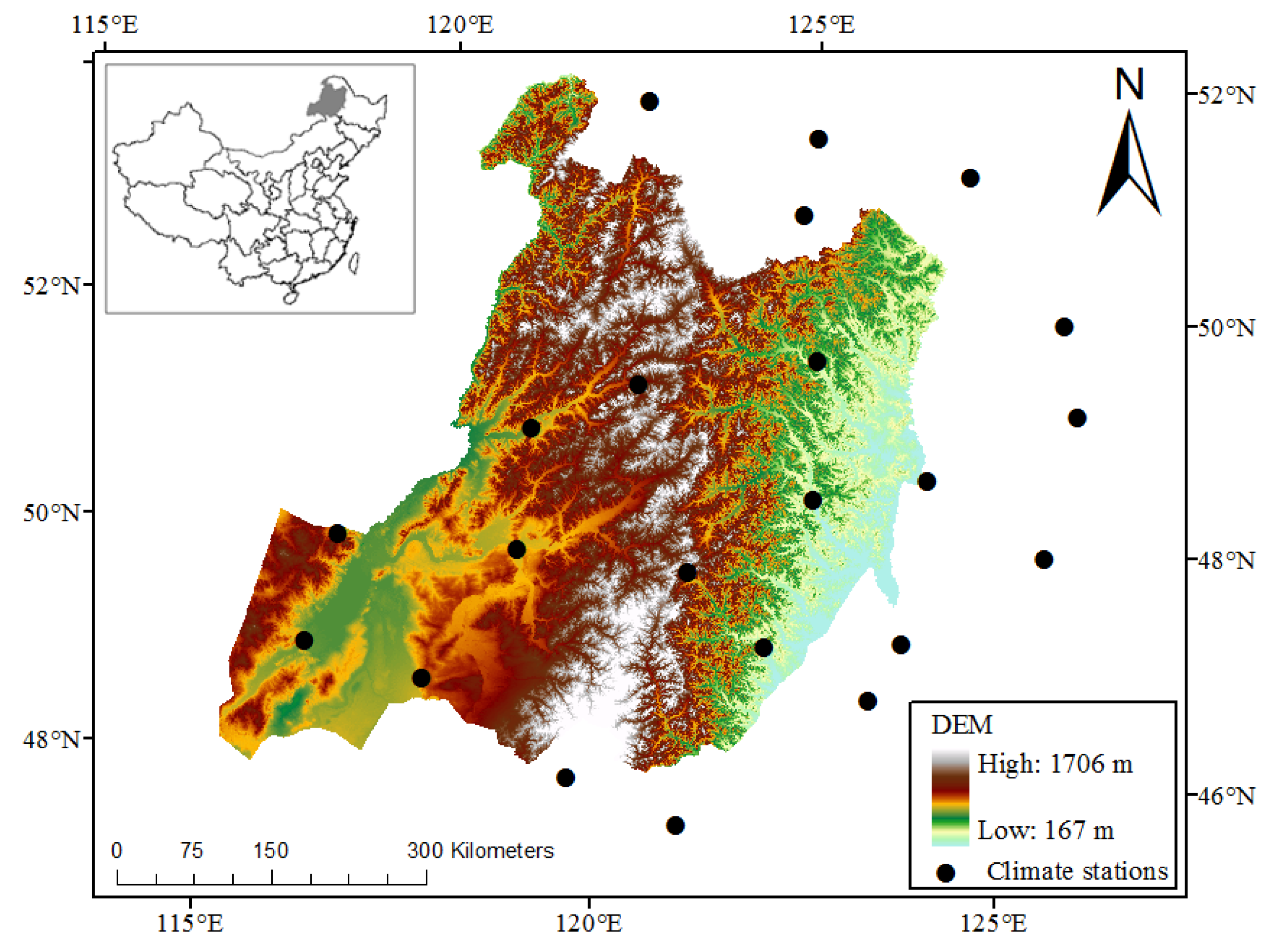
2.1. Study Region

Hulunber (between 47°05′–53°20′N and 115°31′–126°04′E) is located in northeast Inner Mongolia in northeastern China, and covers a total area of approximately 2.53 × 10⁵ km2. Geographically, the region is part of the Mongolian Plateau, and the northeast-southwest-oriented Greater Khingan Range occupies the middle of the Hulunber region. The region can be characterized as a transitional ecotone between the forest ecosystem of the eastern Great Khingan Mountains and plateau steppe of western Inner Mongolia, as well as small areas of farming in the southeast (Figure 1). The climate in this region is governed by a typical continental climate regime with short summers, long winters, and a short frost-free period of only 100–110 days. The Great Khingan Mountains divide the regional climate between a temperate monsoon climate (in the eastern portion) and a temperate continental climate (in the western portion). The annual mean temperature range is −4–4 °C, with temperate ranges of 1.3–2.4 °C in the farming region in the eastern Great Khingan Mountains, −2.0–4.3 °C in the northern forest region, and 0.4–3.0 °C in the western steppe region. The annual precipitation varies widely from 195 mm in the west to 450 mm of the east and primarily falls between July and August. The forest region receives 240–400 mm, the area west of the Great Khingan Mountains receives 200–240 mm, and the area east of the Great Khingan Mountain receives 400–450 mm. The main vegetation types include coniferous forest, broad-leaved forest, shrub, steppe, meadow, and cultivated plants [18].
Figure 1. Spatial patterns in the digital elevation model (DEM) of the Hulunber region.
Remotesensing 07 11914 g001

2.2. GIMMS NDVI3g Data

The NDVI has long been used to monitor terrestrial vegetation dynamics because it is directly related to the photosynthetic capacity and energy absorption of plant canopies [19,20]. In this study, the latest GIMMS NDVI3g product was used. The data (1982–2012) was acquired from the Ecological Forecasting Lab at the NASA Ames Research Center [21] with a consistent time series with a 1/12° (approximately 8 km) spatial and a bi-monthly temporal resolution [14,22]. The product is derived from the AVHRR satellite series 7, 9, 11, 14, 16, 17, 18 and 19 and has been corrected for radiation, geometry, clouds and volcanic aerosols to improve the data quality: It has an improved calibration and improved cloud masking compared to the older versions [14,23]. NDVI3g is the first data set of its kind that is appropriate for long-term studies of land surface trends in vegetation photosynthetic capacity, seasonality or phenology, and climate-vegetation couplings, and it aimed to improve data quality in the high latitudes [24] and is superior in describing the changes in vegetation activity in the Northern Hemisphere [25].

2.3. Climate Data and Auxiliary Data

A climate dataset of monthly mean temperature and monthly precipitation from 18 meteorological stations (black points in Figure 1) across eastern Inner Mongolia and western Heilongjiang province was provided by the China Meteorological Data Sharing Service System [26] for the period of 1982–2012. These monthly climate data were then interpolated and rasterized to a spatial resolution of 8 km in an ArcGIS environment using the Kriging method. Global Land Survey Digital Elevation Model (GLSDEM) data with a resolution of 90 m for the city of Hulunber, published by the Global Land Cover Facility at the University of Maryland in 2008 [27], were obtained to extract topographic information. The vegetation types were obtained from a digitized 1:1,000,000 vegetation map of the People’s Republic of China acquired from the Data Center for Resources and Environmental Sciences, Chinese Academy of Sciences (RESDC) [28].

3. Methods

3.1. NDVI Time Series Pre-Processing

Before extracting the vegetation phenology from the NDVI time-series, an analysis and reconstruction procedure was needed to remove residual atmospherically contaminated and unfavorable sun-sensor-surface viewed pixels in the dataset. Several methods have been developed for this purpose [29,30,31,32,33,34]. The HANTS (Harmonic Analysis of NDVI Time Series) algorithm [32,35] is a harmonic analysis based series reconstruction method, and it has been widely used to process time series NDVI images. This method has been proven globally applicable and appealing for phenological studies [36,37,38,39]. The HANTS algorithm uses Fourier analyses and iterative curve fitting to remove pronounced outliers in a time series that may result from atmospheric conditions or snow cover and then to construct a smooth curve. Thus, the HANTS algorithm was adopted to reconstruct NDVI time series in this study. To correctly reconstruct the time series, the parameters of the HANTS algorithm need to be set carefully. After reviewing various parameter settings used in previous applications [35,38,39,40], the detailed parameters were set in this study and are shown in Table 1. Figure 2 shows the HANTS reconstruction of the NDVI time series, which produced a smoothly varying curve.
Table 1. HANTS parameter settings applied in this study.
ParametersNumber of FrequencySuppression FlagLow ThresholdHigh ThresholdFit Error ToleranceDegree of OverdeterminednessSampling Factor
Values24 (Yearly)Low010.0550.5
Figure 2. Illustration of NDVI (normalized difference vegetation index) time series reconstruction using the HANTS algorithm.
Remotesensing 07 11914 g002

3.2. Determination of Phenological Parameters

Two phenological parameters, the SOS and the EOS were extracted from the NDVI time series using the dynamic threshold method developed by Burgan and Hartford [41]. This method has been widely accepted by ecologists and phenologists for use in phenology studies [5,42,43]. In the dynamic threshold method, the greenness of the vegetation is indexed by transforming the NDVI data into a NDVIratio (with values between 0 and 1) between the NDVI value at a given time [NDVI (t)] and the minimum NDVI value (NDVImin) for the time span of interest, normalized by the total range of NDVI values during this time span (NDVImax −NDVImin) (Equation (1)), the process was implemented per year and per pixel. The SOS is defined as the day of the year (DOY) when the NDVI value exceeds a local threshold NDVIratio, and the EOS is defined as the DOY when the NDVI value drops below the local threshold NDVIratio. Considering the effects of snow cover on the onset vegetation green-up [44,45,46], the threshold was set to one-fifth of the difference between NDVImax and NDVImin (Equation (2)), which was determined from previous literature that applied in the same threshold to different ecosystems [44,47,48,49,50]. The LOS is calculated as the difference between the start and end of the growing season. To minimize the influence of small patches in the phenology extraction, we initially clustered pixels into homogenous clusters using a window size of 5; consequently, the window-averaged NDVI values were used instead of the center pixel values.
N D V I r a t i o = N D V I   ( t ) N D V I m i n N D V I m a x N D V I m i n
V T h r e s h o l d = (   N D V I m a x N D V I m i n ) / 5

3.3. Analysis

Three vegetation groups were created to investigate the temporal variation in vegetation phenology: (a) the steppe region; (b) the forest region; and (c) the agricultural region. The divisions were based on the vegetation types classified in the vegetation map. The steppe region includes meadow steppe, typical steppe, desert steppe, etc. The forest region includes coniferous forest, broad-leaved forest, deciduous forest, etc. In this study, the phenological parameters were analyzed within the different vegetation types. Temporal trends in the vegetation phenology from 1982–2012 were discussed in Section 4.2, which determined using the linear regression between the annual phenological parameters and the year. The response of vegetation phenology to climatic variables was assessed based on the temporal trends in the monthly temperature and precipitation data for the month prior to the phenological parameters. Additionally, the variability in the phenological parameters with time between different vegetation types was also evaluated.

4. Results

4.1. Spatial Patterns in SOS, EOS and LOS

Figure 3 displays the distributions of the SOS, EOS and LOS in the whole Hulunber region averaged from the 30 years during 1982–2012. In Figure 3a, the majority of SOS dates were widely distributed between the 90th Julian day and the 150th Julian day. The SOS of the forest region (approximate 105th Julian day (±5); 10 April–20 April), was later than that of the agricultural region (approximate 95th Julian day (±10); 25 March–15 April). The steppe region had the latest SOS, which occurred on the 115th Julian day (±15) (10 April–10 May). The EOS showed the opposite trend relative to the SOS and is shown in Figure 3b. The EOS dates ranged from the 245th Julian day to the 305th Julian day. The steppe region had the earliest EOS, which was approximately the 259th Julian day (±15) (28 August–30 September), and the EOS of the forest region (the 278th Julian day (±10); 26 September–15 October) was slightly earlier than the agricultural region (279th Julian day (±10); 27 September–16 October). The LOS depended on both the SOS and EOS, and regions with earlier mean SOS dates featured longer LOS values (Figure 3c). The maximum value was observed in Honghuaerji Forest Park, which is the largest sandy Scotch pine forest in Asia. The LOS of the agricultural region (184 ± 15 days) was longer than that of the forest (172 ± 10 days) or steppe regions (144 ± 30 days).
Figure 3. Spatial distribution of phenological parameters in Hulunber during the period 1982–2012. (a) SOS; (b) EOS; (c) LOS.
Remotesensing 07 11914 g003

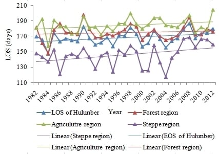
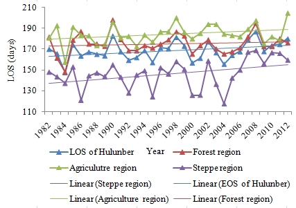
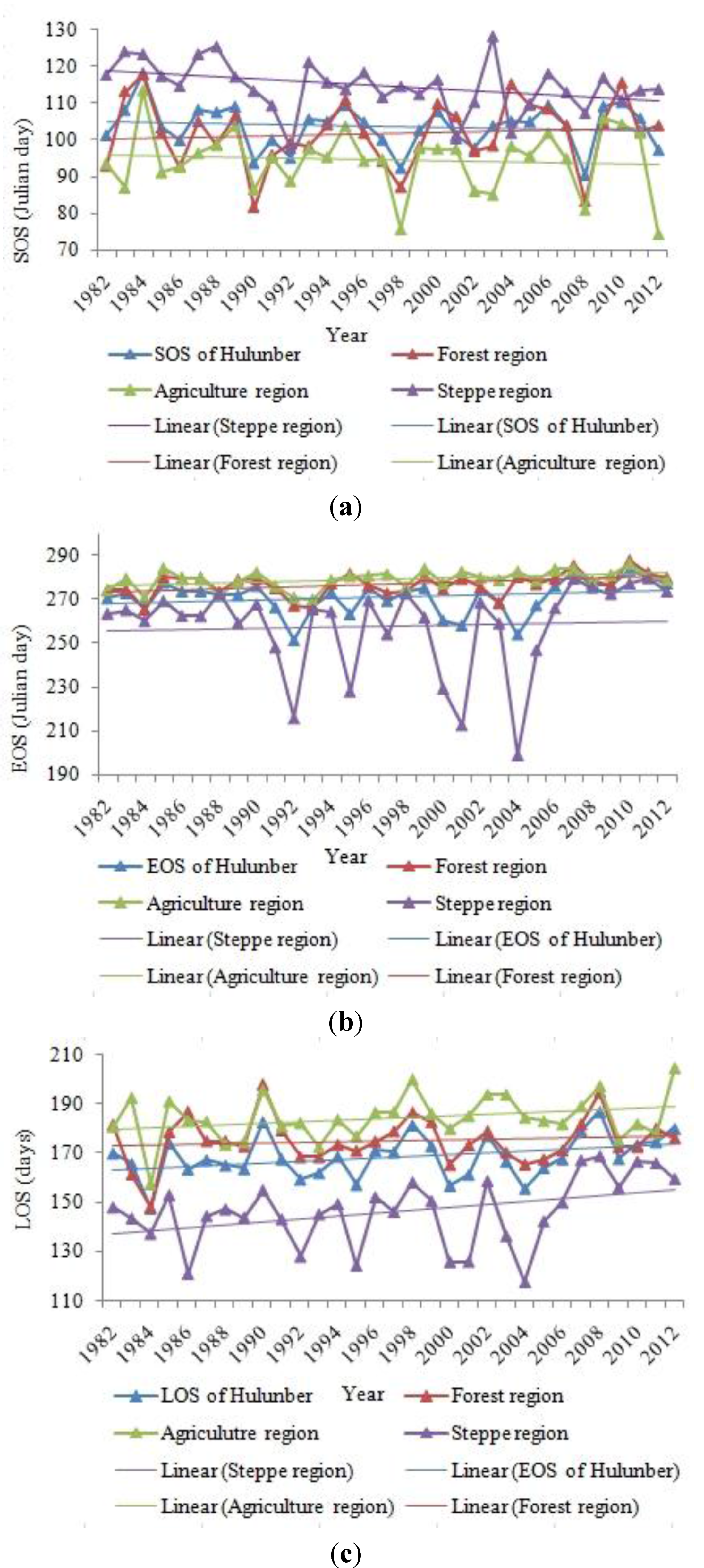
4.2. Temporal Changes in SOS, EOS, LOS

To evaluate the temporal SOS, EOS and LOS trends among the three regions in Hulunber, Figure 4 illustrates the interannual variations of the SOS, EOS and LOS in Hulunber and in its three regions during the period between 1982 and 2012. The SOS trended downward, whereas the LOS trended upward, both of which suggested an earlier spring leaf-out and a longer vegetation growing season. The SOS for the entire study area was 3.30 days earlier in the 2010 than in the 1982. The SOS of the steppe area and farming region advanced by 7.90 days and 2.80 days, respectively, whereas the forested area was delayed by 0.82 days. Additionally, the EOS was delayed by 8.81 days on average during the analysis period. The EOS of the steppe region, forested area and agricultural region advanced by 12.30 days, 9.60 days and 4.51 days, respectively. The opposite long-term trends of the SOS and the EOS led to an increase in the LOS (Figure 4c), with the average LOS of the Hulunber region increasing by an average of 12.11 days between the beginning and end of the analyzed period. The LOS of the steppe region, forest region and agricultural region increased by 4.4 days, 10.42 days and 1.71 days, respectively. The increase in the length of the growing season in the steppe region during 1982–2012 was caused by the earlier SOS and later EOS, and that of the forest region was associated with the later EOS. The lengthened LOS in the agricultural region was caused by both the earlier SOS and the later EOS. Thus, the later EOS was the most significant factor in extending the growing season.

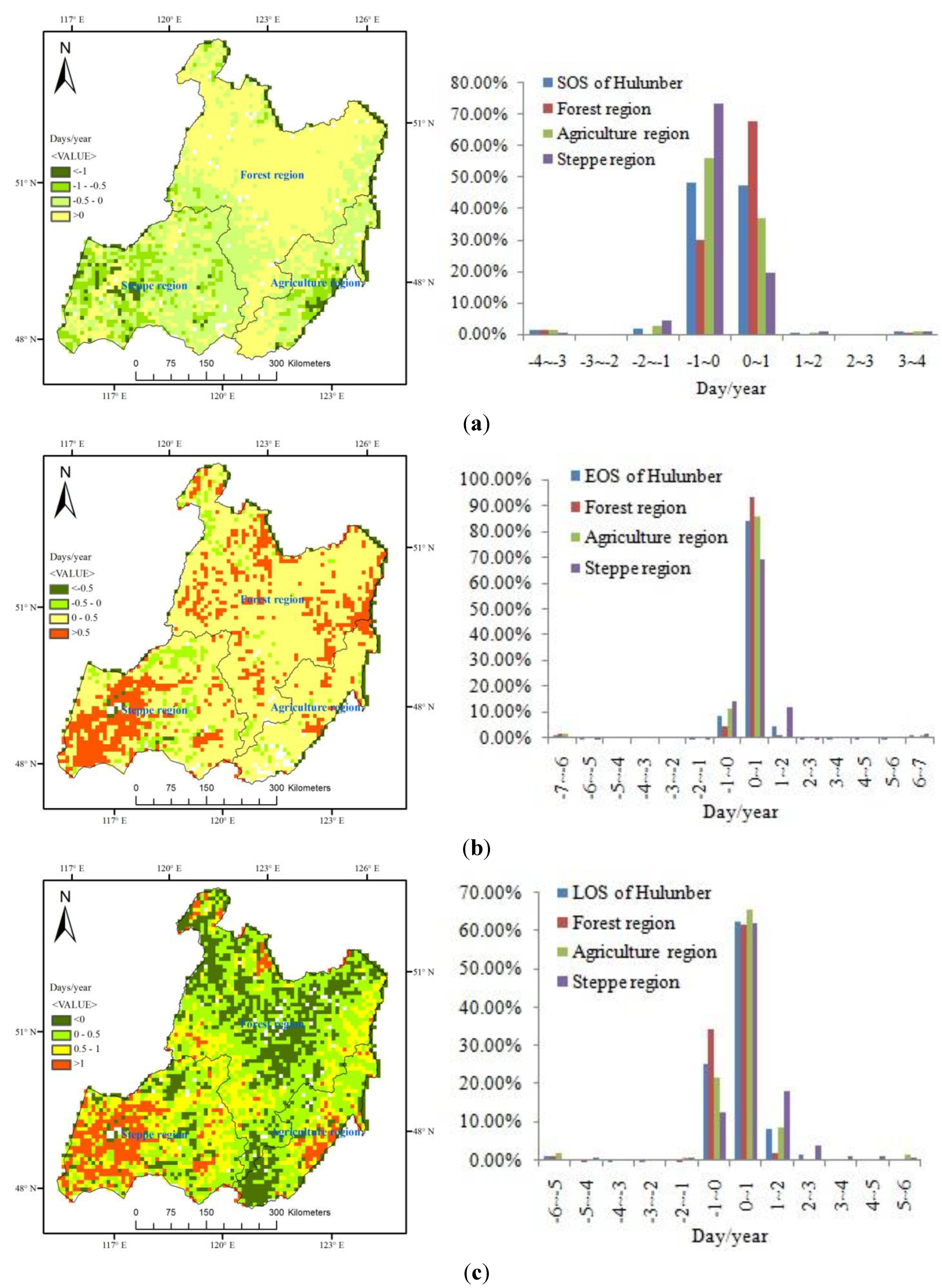
4.3. Variation Ratio in the SOS, EOS, and LOS

To determine the phenology variation ratio, the SOS, EOS and LOS values were divided by the time period of 30 years. Figure 5 shows the spatial distributions of the variation ratios of the SOS, EOS and LOS in Hulunber from 1982–2012. The variations in the SOS were negative in 52% of the whole study region, indicating that half of the region experienced an earlier SOS. The changes in the steppe region were greater than those in the forest and agricultural regions. The SOS date advanced in 79% of the steppe region, 32% of the forest region and 61% of the agricultural region. The advanced SOS distributed around Hulun Lake may have been caused by changes in land use or by the interannual variability in precipitation. The changes in the SOS of the steppe region and agricultural region were mainly in the range of −0.5–0 days/yr. Overall, 91% of the entire region exhibited later autumn leaf loss, and 84% of the steppe region exhibited a later EOS. In the other two regions, 95% of the forest region and 87% of the agricultural region exhibited later autumn leaf loss. The LOS increased in 74% of the study region. The LOS decreased in 36% of the forest region and 24% of the agricultural region but increased in 25% of the steppe region by more than 1 day/yr.

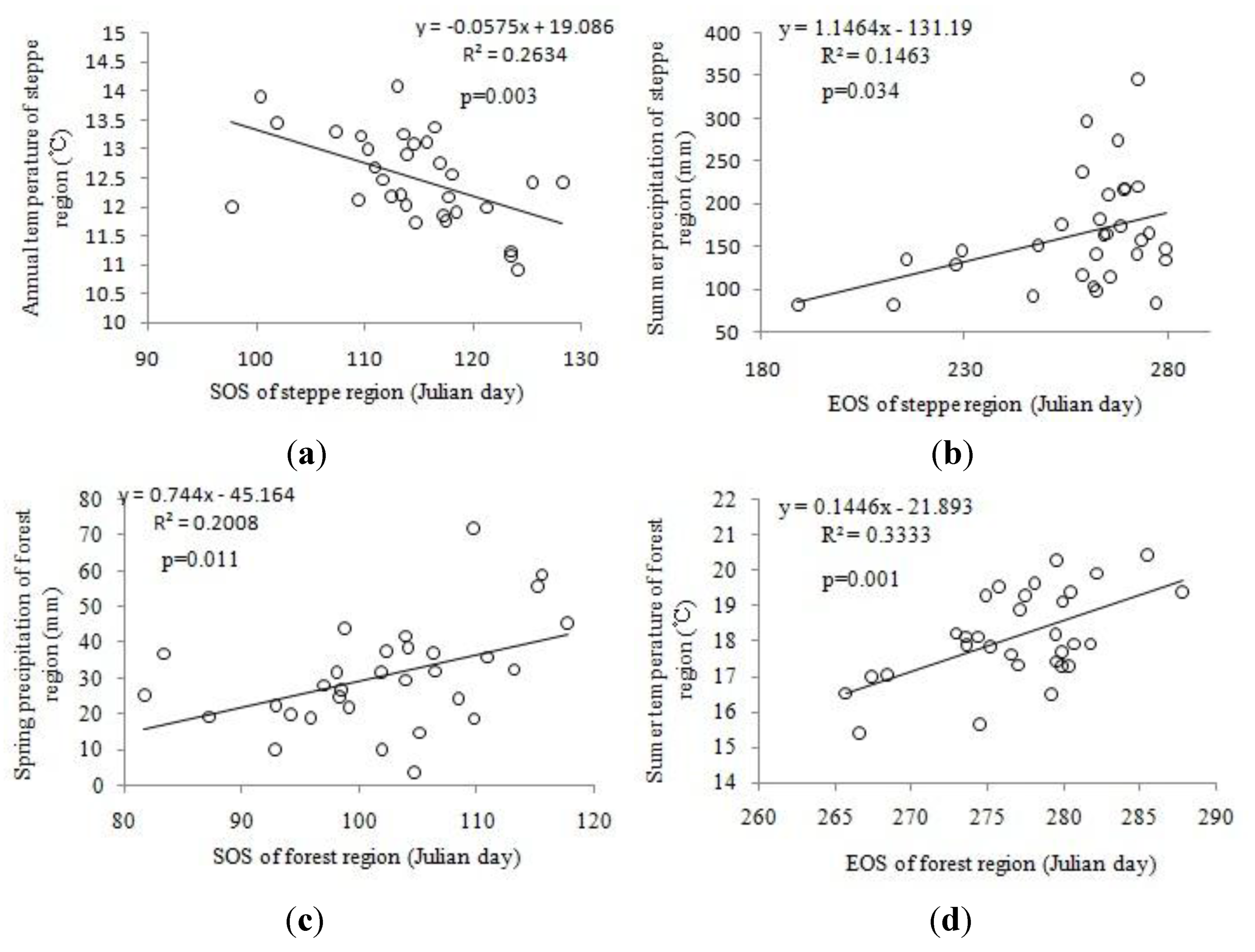
4.4. Relationships between Phenology and Climate

To explore the variability in the three phenological parameters (SOS, EOS, and LOS) in relation to climatic factors, we compared the average SOS, EOS, and LOS values in the steppe region, forest region and agricultural region, with 14 climatic factors (annual precipitation, annual temperature, seasonal precipitation, seasonal temperature, seasonal cumulative temperature above 10 °C, and seasonal cumulative temperature above 0 °C. The seasons were defined as spring (April–May), summer (June–August), and autumn (September–October)).
Figure 4. Interannual phenology variability in the growing season (April–October) for the three main regions and the entire Hulunber area from 1982 to 2012. (a) SOS; (b) EOS; (c) LOS.
Remotesensing 07 11914 g004
Figure 5. Spatial distributions of the variation ratio in Hulunber during 1982–2012. (a) SOS; (b) EOS; (c) LOS.
Remotesensing 07 11914 g005
For the steppe region we found that the correlation coefficients (CCs) between the SOS and the spring precipitation, annual temperature, and spring cumulative temperature above 0 °C are stronger than between the SOS and the other factors (Table 2). Among these three factors, the correlation between the annual temperature and the SOS is the strongest (Figure 6a, CC = −0.513, P = 0.003), suggesting that a warmer year would result in the advance of the SOS. A spring cumulative temperature above 0 °C also affects the steppe green-up. Additionally, a significant correlation between the summer precipitation and the EOS was found (Figure 6b, CC=0.382, P=0.034), and the correlation between the summer temperature and the EOS is also notable (CC = −0.399, P = 0.032). These observations indicate that greater summer precipitation and lower summer temperatures are correlated with later steppe EOS dates. Interestingly, the annual precipitation and the summer precipitation are the most influential factors for the LOS.
Table 2. Correlation coefficients between phenological parameters and climatic factors in the steppe region.
SOSEOSLOS
Annual precipitation0.3200.364 *0.430 **
Spring precipitation−0.411 * 0.165
Summer precipitation 0.382 *0.493 **
Autumn precipitation 0.0310.070
Annual temperature−0.513 **−0.1530.161
Spring temperature−0.179 0.311 *
Summer temperature −0.399 *0.011
Autumn temperature −0.329−0.007
Spring cumulative temperature above 10 °C−0.230 0.411 *
Summer cumulative temperature above 10 °C −0.240−0.120
Autumn cumulative temperature above 10 °C −0.280−0.123
Spring cumulative temperature above 0 °C−0.479 ** 0.013
Summer cumulative temperature above 0 °C −0.0270.034
Autumn cumulative temperature above 0 °C −0.330−0.021
* P < 0.05; ** P < 0.01.
In the forest region, a significant correlation between the SOS and the spring precipitation (Table 3; Figure 6c, CC = 0.448, P = 0.011) was found, and a negative correlation exists between the SOS and the spring mean temperature (CC = −0.388, P = 0.031). These correlations confirmed that the precipitation and temperature in the spring are the main factors influencing forest green-up and that less rainfall and warmer springs lead to earlier SOS dates. The correlation coefficient between the EOS and the summer temperature is the strongest (Figure 6d, CC = 0.577, P = 0.001), and the correlations between the EOS and the summer precipitation and summer cumulative temperature above 10 °C are also significant. In the forest region, the summer temperature was the main factor driving the delay in the EOS, and the summer precipitation also contributed to the variations in the EOS. For the LOS, the annual temperature was the most influential factor, and precipitation appeared to have only a slight effect on the LOS variation in the forest region.
Table 3. Correlation coefficients between phenological parameters and climatic factors in the forest region.
SOSEOSLOS
Annual precipitation−0.408 *−0.320−0.145
Spring precipitation0.448 * −0.299
Summer precipitation −0.513 **−0.022
Autumn precipitation −0.3220.071
Annual temperature−0.0610.403 *0.449 **
Spring temperature−0.388 * 0.302
Sumer temperature 0.577 **0.474 **
Autumn temperature 0.2660.006
Spring cumulative temperature above 10 °C−0.162 0.153
Summer cumulative temperature above 10 °C 0.516 **0.444 *
Autumn cumulative temperature above 10 °C 0.096−0.126
Spring cumulative temperature above 0 °C−0.285 0.282
Summer cumulative temperature above 0 °C 0.514 **0.456 *
Autumn cumulative temperature above 0 °C 0.2920.131
* P < 0.05; ** P < 0.01.
Figure 6. Relationships between phenological parameters and climatic variables for two regions of the study area. (a) SOS of the steppe region; (b) EOS of the steppe region; (c) SOS of the forest region; (d) EOS of the forest region.
Remotesensing 07 11914 g006
In the agricultural region (Table 4), no significant correlations existed between the phenological parameters and climatic factors. However, several weak relationships are observed, such as between the spring temperature and the SOS, the summer precipitation and the EOS, and the summer cumulative temperature above 10 °C and the EOS. These observations indicate that precipitation was not the driving factor of the variability in the phenology. The temperature may more significantly influence the variations in the phenology. We believe that the phenology of the agricultural region in Hulunber is primarily related to human disturbances, and it might have been a result of ecological projects by the Chinese government, such as Grain for Green, the Natural Forest Conversion Program and the Beijing-Tianjin Sand Source Control Program.
Table 4. Correlation coefficients between phenological parameters and climatic factors in the agricultural region.
SOSEOSLOS
Annual precipitation−0.250−0.406 *0.021
Spring precipitation−0.002 −0.020
Summer precipitation 0.3220.158
Autumn precipitation 0.166−0.104
Annual temperature−0.150−0.3040.292
Spring temperature−0.362 * 0.331
Summer temperature −0.3430.174
Autumn temperature −0.1850.192
Spring cumulative temperature above 10 °C−0.332 −0.201
Summer cumulative temperature above 10 °C −0.380 *0.124
Autumn cumulative temperature above 10 °C −0.1040.105
Spring cumulative temperature above 0 °C−0.356 −0.356
Summer cumulative temperature above 0 °C −0.371 *0.135
Autumn cumulative temperature above 0 °C −0.234−0.038
* P < 0.05; ** P < 0.01.
Our results showed that in the steppe region, both the temperature and the precipitation led to a lengthened LOS. However, in the forest region, longer durations of vegetation growth were more closely correlated with the temperature than the precipitation. The rate of temperature increase in Hulunber was 0.025 °C/yr, with spring temperatures increasing by 0.016 °C/yr and autumn temperatures increasing by 0.051 °C/yr. Our results also suggest that warmer spring temperatures trigger earlier vegetation green-up dates at a rate of 6.96 days/°C, and warmer autumn temperatures cause later EOS dates at a rate of 5.76 days/°C.

5. Discussion

5.1. Comparison with Previous Studies

Previous studies using the NDVI time series dataset from AVHRR or MODIS show long-lasting LOS trends in the Inner Mongolia steppe [51], China [10], Africa [3] and Europe [22,52]. Zhou et al. [53] analyzed NDVI data from 1981–1999 and found that north of 40°N in Eurasia, the vegetation growing season was extended nearly 18 days, with spring beginning a week earlier and autumn ending 10 days later. Miao et al. [54] analyzed the phenology in the Mongolian Plateau through an inter-comparison of global vegetation datasets: they found that the temporal average SOS showed no significant “earlier spring” onset during 1982–2012 in the middle and northern Mongolian Plateau. Zhang et al. [2] merged GIMMS-based SOS from 1982 to 2000 with SPOT-VGT-based SOS from 2001 to 2011 in the Tibetan Plateau, which showed an advancing SOS trend at a rate of 1.04 d/y from 1982 to 2011. He et al. [55] analyzed the vegetation phenological variation and the relationship with the climatic factors using MODIS NDVI data of Zhejiang province. The results showed that the average LOS was approximately 222 days, SOS displayed a non-significant advancing trend, and the EOS was significantly delayed. The correlation analysis of phenological metrics and climatic factors indicated that SOS and EOS were positively related with mean temperature, whereas precipitation and the humidity index were negatively correlated, though not significant. Myneni et al. [5] and Cayan et al. [56] analyzed the relationship between temperature and LOS, and their results showed that warmer springs in 1980s enabled earlier onsets of plant growth and longer growing seasons in the Northern Hemisphere mid- and high-latitudes. Those studies indicated that LOS was extended in recent years, a change that was more closely correlated with temperature than with precipitation [57,58]. Jeong et al. [58] also reported that the correlation of the extended growing season with autumn temperatures was greater than with spring temperature. In our results, the vegetation growing season was extended 12.11 days, with 3.30 days from a slightly early spring and 8.81 days attributed to a late autumn. The correlation analysis of phenological metrics and climatic factors indicated that both temperature and precipitation led to a lengthened LOS in the steppe area and forest region, and warmer spring temperatures trigger earlier vegetation green-up dates at a rate of 6.96 days/°C, and warmer autumn temperatures cause later EOS dates at a rate of 5.76 days/°C.
Most of the changes in the growing seasons during 1982–2012 were generally consistent with previous research. However, many studies have shown that both earlier spring leafing and later autumn senescence were factors [10,59] that led to the extended growing season. Our research indicated that the later EOS date was the most significant factor in extending the growing season during 1982–2012 in Hulunber, thus longer-lasting vegetation growth in the research years can be attributed to extended leaf senescence.

5.2. Study Limitations

Uncertainty in our results may result from the reconstructed time series processed by the HANTS algorithm. Several models have been developed in the past to smooth and reconstruct time series vegetation index data, and differences between the models and fine tuning of model parameters lead to potential differences, uncertainty and bias between the results amongst users [29,60]. Thus, a comparative analysis of the differences between these methods in Hulunber must be further performed.
This research must also be expanded to a deeper discussion of the response of phenological variation to climate change. In this study, we only used simple relationships between the phenological and climatic parameters, such as mean temperature and precipitation, to examine changes in LOS related to climate change. Therefore, they reflect only spatial correlations. However, to draw conclusions about phenological changes under a changing climate conditions, it would be much more valuable to analyze temporal correlations. This study also does not consider the effects of latitude [61], solar radiation changes, land use and land cover changes [62], rising atmospheric CO2 concentrations, water controls [7] or the unexpected role of winter precipitation [63], among other factors, and these factors will be addressed in follow-up studies.

6. Conclusions

In this study, the latest GIMMS NDVI3g dataset which has high quality data for the high latitudes [24], was used in Hulunber, China, from 1982 to 2012. The start date of the growing season (SOS), the end date of the growing season (EOS) and the length of growing season (LOS) were derived from this time series using a dynamic threshold method to describe the distribution and variability of vegetation phenology in the study area, and three ecosystem regions were classified in the study region: the steppe region, forest region, and agricultural region. The response of the variations in phenology to climate change in the three eco-regions was also discussed. The results indicated that Hulunber experienced obvious phenological variation over the past three decades, including a 12.1-day increase in the LOS, a 3.3-day advance of SOS and an 8.8-day delay of EOS. However, the steppe, forest and agricultural regions presented different variation patterns, with the LOS of the steppe, forest and agricultural regions increased by 4.4 days, 10.42 days and 1.71 days, respectively. The later EOS was found to be the most significant factor in extending the growing season. Furthermore, temperature and precipitation were closely correlated with the variations in the phenology. The correlation analysis of the phenological metrics and climatic factors indicated that both temperature and precipitation led to a lengthened LOS in the steppe area and forest region, and warmer spring temperatures trigger earlier vegetation green-up dates at a rate of 6.96 days/°C, and warmer autumn temperatures cause later EOS dates at a rate of 5.76 days/°C. This study provides a useful understanding of the recent changes in phenology and its variability in this high-latitude study area, and details the responses of several ecosystems to climate change.

Acknowledgments

We gratefully acknowledge Ruirui Yan whose comments lead to significant improvements in this manuscript. We also acknowledge data support from the Agricultural Data Center (http://www.agridata.cn) and financial support of the Key Technologies Research and Development Program of China (2012BAC19B04, 2013BAC03B02), the International Science and Technology Cooperation Project of China (2012DFA31290) and the support of China Agriculture Research System.

Author Contributions

All authors made great contributions to the work. Huan Tang and Zhenwang Li performed the analyses and prepared the paper. Xiaoping Xin and Zhiliang Zhu provided the technical guidance and contributed to the discussion. Baohui Zhang and Baorui Chen assisted with data collection and image analysis.

Conflicts of Interest

The authors declare no conflict of interest.

References

  1. Jeong, S.J.; Ho, C.H.; GIM, H.J.; Brown, M.E. Phenology shifts at start vs. end of growing season in temperate vegetation over the Northern Hemisphere for the period 1982–2008. Glob. Chang. Biol. 2011, 17, 2385–2399. [Google Scholar] [CrossRef]
  2. Zhang, G.; Zhang, Y.; Dong, J.; Xiao, X. Green-up dates in the Tibetan plateau have continuously advanced from 1982 to 2011. Proc. Natl. Acad. Sci. 2013, 110, 4309–4314. [Google Scholar] [CrossRef] [PubMed]
  3. Vrieling, A.; de Leeuw, J.; Said, M.Y. Length of growing period over Africa: Variability and trends from 30 years of ndvi time series. Remote Sens. 2013, 5, 982–1000. [Google Scholar] [CrossRef]
  4. Fu, Y.H.; Piao, S.; de Beeck, M.O.; Cong, N.; Zhao, H.; Zhang, Y.; Menzel, A.; Janssens, I.A. Recent spring phenology shifts in western central Europe based on multiscale observations. Glob. Ecol. Biogeogr. 2014, 23, 1255–1263. [Google Scholar] [CrossRef]
  5. Myneni, R.B.; Keeling, C.; Tucker, C.; Asrar, G.; Nemani, R. Increased plant growth in the northern high latitudes from 1981 to 1991. Nature 1997, 386, 698–702. [Google Scholar] [CrossRef]
  6. Walther, G.-R.; Post, E.; Convey, P.; Menzel, A.; Parmesan, C.; Beebee, T.J.; Fromentin, J.-M.; Hoegh-Guldberg, O.; Bairlein, F. Ecological responses to recent climate change. Nature 2002, 416, 389–395. [Google Scholar] [CrossRef] [PubMed]
  7. Forkel, M.; Migliavacca, M.; Thonicke, K.; Reichstein, M.; Schaphoff, S.; Weber, U.; Carvalhais, N. Co-dominant water control on global inter-annual variability and trends in land surface phenology and greenness. Glob. Chang. Biol. 2015. [Google Scholar] [CrossRef] [PubMed]
  8. Piao, S.; Friedlingstein, P.; Ciais, P.; Viovy, N.; Demarty, J. Growing season extension and its impact on terrestrial carbon cycle in the Northern Hemisphere over the past 2 decades. Glob. Biogeochem. Cycles 2007, 21, GB3018. [Google Scholar] [CrossRef]
  9. Jeganathan, C.; Dash, J.; Atkinson, P. Remotely sensed trends in the phenology of northern high latitude terrestrial vegetation, controlling for land cover change and vegetation type. Remote Sens. Environ. 2014, 143, 154–170. [Google Scholar] [CrossRef]
  10. Piao, S.; Fang, J.; Zhou, L.; Ciais, P.; Zhu, B. Variations in satellite-derived phenology in China's temperate vegetation. Glob. Chang. Biol. 2006, 12, 672–685. [Google Scholar] [CrossRef]
  11. De Beurs, K.M.; Henebry, G.M. Land surface phenology and temperature variation in the international geosphere-biosphere program high-latitude transects. Glob. Chang. Biol. 2005, 11, 779–790. [Google Scholar] [CrossRef]
  12. De Beurs, K.M.; Henebry, G.M. Spatio-temporal statistical methods for modelling land surface phenology. In Phenological Research; Springer: Dordrecht, The Netherlands, 2010; pp. 177–208. [Google Scholar]
  13. White, M.A.; De Beurs, K.M.; Didan, K.; Inouye, D.W.; Richardson, A.D.; Jensen, O.P.; O’Keefe, J.; Zhang, G.; Nemani, R.R.; Van Leeuwen, W.J.D.; De Wit, A.; et al. Intercomparison, interpretation, and assessment of spring phenology in north America estimated from remote sensing for 1982–2006. Glob. Chang. Biol. 2009, 15, 2335–2359. [Google Scholar]
  14. Pinzon, J.E.; Tucker, C.J. A non-stationary 1981–2012 AVHRR NDVI3g time series. Remote Sens. 2014, 6, 6929–6960. [Google Scholar] [CrossRef]
  15. Wang, J.; Dong, J.; Liu, J.; Huang, M.; Li, G.; Running, S.W.; Smith, W.K.; Harris, W.; Saigusa, N.; Kondo, H. Comparison of gross primary productivity derived from GIMMS NDVI3g, GIMMS, and MODIS in southeast Asia. Remote Sens. 2014, 6, 2108–2133. [Google Scholar] [CrossRef]
  16. Zeng, F.-W.; Collatz, G.J.; Pinzon, J.E.; Ivanoff, A. Evaluating and quantifying the climate-driven interannual variability in global inventory modeling and mapping studies (GIMMS) normalized difference vegetation index (NDVI3g) at global scales. Remote Sens. 2013, 5, 3918–3950. [Google Scholar] [CrossRef]
  17. Høgda, K.A.; Tømmervik, H.; Karlsen, S.R. Trends in the start of the growing season in Fennoscandia 1982–2011. Remote Sens. 2013, 5, 4304–4318. [Google Scholar] [CrossRef]
  18. Wang, X.; Zhao, H. Inner Mongolia Hulun Buir City Agricultural Climate Resources and Division of Forestry and Animal Husbandry; China Meteorological Press: Beijing, China, 2006. [Google Scholar]
  19. Sellers, P.J. Canopy reflectance, photosynthesis and transpiration. Int. J. Remote Sens. 1985, 6, 1335–1372. [Google Scholar] [CrossRef]
  20. Myneni, R.B.; Hall, F.G.; Sellers, P.J.; Marshak, A.L. The interpretation of spectral vegetation indexes. IEEE Trans. Geosci. Remote Sens. 1995, 33, 481–486. [Google Scholar] [CrossRef]
  21. Ecological Forecasting Lab at the NASA Ames Research Center. Available online: http://ecocast.arc.nasa.gov (accessed on 18 March 2015).
  22. Atzberger, C.; Klisch, A.; Mattiuzzi, M.; Vuolo, F. Phenological metrics derived over the European continent from NDVI3g data and MODIS time series. Remote Sens. 2014, 6, 257–284. [Google Scholar] [CrossRef]
  23. Jiang, N.; Zhu, W.; Zheng, Z.; Chen, G.; Fan, D. A comparative analysis between GIMMS NDVIg and NDVI3g for monitoring vegetation activity change in the northern hemisphere during 1982–2008. Remote Sens. 2013, 5, 4031–4044. [Google Scholar] [CrossRef]
  24. Zhu, Z.; Bi, J.; Pan, Y.; Ganguly, S.; Anav, A.; Xu, L.; Samanta, A.; Piao, S.; Nemani, R.R.; Myneni, R.B. Global data sets of vegetation leaf area index (LAI) 3g and fraction of photosynthetically active radiation (FPAR) 3g derived from global inventory modeling and mapping studies (GIMMS) normalized difference vegetation index (NDVI3g) for the period 1981 to 2011. Remote Sens. 2013, 5, 927–948. [Google Scholar]
  25. Xu, L.; Myneni, R.; Chapin, F., III; Callaghan, T.; Pinzon, J.; Tucker, C.; Zhu, Z.; Bi, J.; Ciais, P.; Tømmervik, H. Temperature and vegetation seasonality diminishment over northern lands. Nat. Clim. Chang. 2013, 3, 581–586. [Google Scholar]
  26. China Meteorological Data Sharing Service System. Available online: http://cdc.cma.gov.cn (accessed on 10 January 2015).
  27. Global Land Cover Facility at the University of Maryland. Available online: http://glcf.umd.edu/data/ (accessed on 18 May 2014).
  28. Data Center for Resources and Environmental Sciences, Chinese Academy of Sciences. Available online: http://www.resdc.cn (accessed on 21 September 2014).
  29. Geng, L.; Ma, M.; Wang, X.; Yu, W.; Jia, S.; Wang, H. Comparison of eight techniques for reconstructing multi-satellite sensor time-series NDVI data sets in the Heihe river basin, China. Remote Sens. 2014, 6, 2024–2049. [Google Scholar] [CrossRef]
  30. Lu, X.; Liu, R.; Liu, J.; Liang, S. Removal of noise by wavelet method to generate high quality temporal data of terrestrial MODIS products. Photogramm. Eng. Remote Sens. 2007, 73, 1129–1139. [Google Scholar] [CrossRef]
  31. Fischer, A. A model for the seasonal variations of vegetation indices in coarse resolution data and its inversion to extract crop parameters. Remote Sens. Environ. 1994, 48, 220–230. [Google Scholar] [CrossRef]
  32. Menenti, M.; Azzali, S.; Verhoef, W.; Van Swol, R. Mapping agroecological zones and time lag in vegetation growth by means of fourier analysis of time series of NDVI images. Adv. Space Res. 1993, 13, 233–237. [Google Scholar] [CrossRef]
  33. Chen, J.; Jönsson, P.; Tamura, M.; Gu, Z.; Matsushita, B.; Eklundh, L. A simple method for reconstructing a high-quality NDVI time-series data set based on the savitzky-golay filter. Remote Sens. Environ. 2004, 91, 332–344. [Google Scholar] [CrossRef]
  34. Viovy, N.; Arino, O.; Belward, A. The best index slope extraction (bise): A method for reducing noise in NDVI time-series. Int. J. Remote Sens. 1992, 13, 1585–1590. [Google Scholar] [CrossRef]
  35. Roerink, G.; Menenti, M.; Verhoef, W. Reconstructing cloudfree NDVI composites using fourier analysis of time series. Int. J. Remote Sens. 2000, 21, 1911–1917. [Google Scholar] [CrossRef]
  36. De Jong, R.; de Bruin, S.; de Wit, A.; Schaepman, M.E.; Dent, D.L. Analysis of monotonic greening and browning trends from global NDVI time-series. Remote Sens. Environ. 2011, 115, 692–702. [Google Scholar] [CrossRef] [Green Version]
  37. Azzali, S.; Menenti, M. Mapping vegetation-soil-climate complexes in southern Africa using temporal fourier analysis of NOAA-AVHRR NDVI data. Int. J. Remote Sens. 2000, 21, 973–996. [Google Scholar] [CrossRef]
  38. Zhou, J.; Jia, L.; Menenti, M. Reconstruction of global MODIS NDVI time series: Performance of harmonic analysis of time series (HANTS). Remote Sens. Environ. 2015, 163, 217–228. [Google Scholar] [CrossRef]
  39. Julien, Y.; Sobrino, J.A. Comparison of cloud-reconstruction methods for time series of composite NDVI data. Remote Sens. Environ. 2010, 114, 618–625. [Google Scholar] [CrossRef]
  40. Verhegghen, A.; Bontemps, S.; Defourny, P. A global NDVI and EVI reference data set for land-surface phenology using 13 years of daily SPOT-vegetation observations. Int. J. Remote Sens. 2014, 35, 2440–2471. [Google Scholar] [CrossRef]
  41. Burgan, R.E.; Hartford, R.A. Monitoring Vegetation Greenness with Satellite Data; US Department of Agriculture, Forest Service, Intermountain Research Station: Ogden, UT, USA, 1993; Vol. 297, p. 13. [Google Scholar]
  42. White, M.A.; Thornton, P.E.; Running, S.W. A continental phenology model for monitoring vegetation responses to interannual climatic variability. Glob. Biogeochem. Cycles 1997, 11, 217–234. [Google Scholar] [CrossRef]
  43. Wang, Q.; Tenhunen, J.; Dinh, N.Q.; Reichstein, M.; Vesala, T.; Keronen, P. Similarities in ground-and satellite-based NDVI time series and their relationship to physiological activity of a scots pine forest in Finland. Remote Sens. Environ. 2004, 93, 225–237. [Google Scholar] [CrossRef]
  44. Yu, H.; Luedeling, E.; Xu, J. Winter and spring warming result in delayed spring phenology on the Tibetan plateau. Proc. Natl. Acad. Sci. USA 2010, 107, 22151–22156. [Google Scholar] [CrossRef] [PubMed]
  45. Delbart, N.; Kergoat, L.; Le Toan, T.; Lhermitte, J.; Picard, G. Determination of phenological dates in boreal regions using normalized difference water index. Remote Sens. Environ. 2005, 97, 26–38. [Google Scholar] [CrossRef]
  46. Shen, M.; Zhang, G.; Cong, N.; Wang, S.; Kong, W.; Piao, S. Increasing altitudinal gradient of spring vegetation phenology during the last decade on the Qinghai-tibetan plateau. Agric. For. Meteorol. 2014, 189, 71–80. [Google Scholar] [CrossRef]
  47. Van Leeuwen, W.J. Monitoring the effects of forest restoration treatments on post-fire vegetation recovery with MODIS multitemporal data. Sensors 2008, 8, 2017–2042. [Google Scholar] [CrossRef]
  48. Jönsson, P.; Eklundh, L. Seasonality extraction by function fitting to time-series of satellite sensor data. IEEE Trans. Geosci. Remote Sens. 2002, 40, 1824–1832. [Google Scholar] [CrossRef]
  49. Liu, L.L.; Liu, L.Y.; Hu, Y. Comparative analysis of global vegetation phenology based on AVHRR and MODIS. Remote Sens. Technol. Appl. 2012, 5, 017. [Google Scholar]
  50. Zhao, J.J.; Liu, L.Y. Effects of phenological change on ecosystem productivity of temperate deciduous broadleaved forests in north America. Chin. J. Plant Ecol. 2012, 36, 363–371. [Google Scholar] [CrossRef]
  51. Lee, R.; Yu, F.; Price, K.; Ellis, J.; Shi, P. Evaluating vegetation phenological patterns in Inner Mongolia using NDVI time-series analysis. Int. J. Remote Sens. 2002, 23, 2505–2512. [Google Scholar] [CrossRef]
  52. Stöckli, R.; Vidale, P.L. European plant phenology and climate as seen in a 20-year AVHRR land-surface parameter dataset. Int. J. Remote Sens. 2004, 25, 3303–3330. [Google Scholar] [CrossRef]
  53. Zhou, L.; Tucker, C.J.; Kaufmann, R.K.; Slayback, D.; Shabanov, N.V.; Myneni, R.B. Variations in northern vegetation activity inferred from satellite data of vegetation index during 1981 to 1999. J. Geophys. Res.: Atmos. 2001, 106, 20069–20083. [Google Scholar] [CrossRef]
  54. Miao, L.; Luan, Y.; Luo, X.; Liu, Q.; Moore, J.C.; Nath, R.; He, B.; Zhu, F.; Cui, X. Analysis of the phenology in the mongolian plateau by inter-comparison of global vegetation datasets. Remote Sens. 2013, 5, 5193–5208. [Google Scholar] [CrossRef]
  55. He, Y.; Fan, G.F.; Zhang, X.W.; Li, Z.Q.; Gao, D.W. Vegetation phenological variation and its response to climate changes in Zhejiang province. J. Nat. Resour. 2013, 2, 220–233. [Google Scholar]
  56. Cayan, D.R.; Dettinger, M.D.; Kammerdiener, S.A.; Caprio, J.M.; Peterson, D.H. Changes in the onset of spring in the western United States. Bull. Am. Meteorol. Soc. 2001, 82, 399–415. [Google Scholar] [CrossRef]
  57. Cong, N.; Wang, T.; Nan, H.; Ma, Y.; Wang, X.; Myneni, R.B.; Piao, S. Changes in satellite-derived spring vegetation green-up date and its linkage to climate in China from 1982 to 2010: A multimethod analysis. Glob. Chang. Biol. 2013, 19, 881–891. [Google Scholar] [CrossRef] [PubMed]
  58. Jeong, S.J.; Ho, C.H.; Park, T.W.; Kim, J.; Levis, S. Impact of vegetation feedback on the temperature and its diurnal range over the Northern Hemisphere during summer in a 2 × CO2 climate. Clim. Dyn. 2011, 37, 821–833. [Google Scholar] [CrossRef]
  59. Vitasse, Y.; François, C.; Delpierre, N.; Dufrêne, E.; Kremer, A.; Chuine, I.; Delzon, S. Assessing the effects of climate change on the phenology of European temperate trees. Agric. For. Meteorol. 2011, 151, 969–980. [Google Scholar] [CrossRef]
  60. Atkinson, P.M.; Jeganathan, C.; Dash, J.; Atzberger, C. Inter-comparison of four models for smoothing satellite sensor time-series data to estimate vegetation phenology. Remote Sens. Environ. 2012, 123, 400–417. [Google Scholar] [CrossRef]
  61. Zhang, X.; Friedl, M.A.; Schaaf, C.B.; Strahler, A.H.; Liu, Z. Monitoring the response of vegetation phenology to precipitation in Africa by coupling modis and TRMM instruments. J. Geophys. Res.: Atmos. 2005, 110, D12103. [Google Scholar] [CrossRef]
  62. De Beurs, K.M.; Henebry, G.M. Land surface phenology, climatic variation, and institutional change: Analyzing agricultural land cover change in Kazakhstan. Remote Sens. Environ. 2004, 89, 497–509. [Google Scholar] [CrossRef]
  63. Fu, Y.H.; Piao, S.; Zhao, H.; Jeong, S.J.; Wang, X.; Vitasse, Y.; Ciais, P.; Janssens, I.A. Unexpected role of winter precipitation in determining heat requirement for spring vegetation green-up at northern middle and high latitudes. Glob. Chang. Biol. 2014, 20, 3743–3755. [Google Scholar] [CrossRef] [PubMed]

