
Developing Theoretical Marine Habitat Suitability Models from Remotely-Sensed Data and Traditional Ecological Knowledge


Abstract
:
1. Introduction
2. Methods
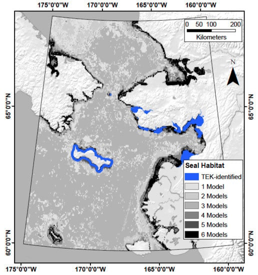
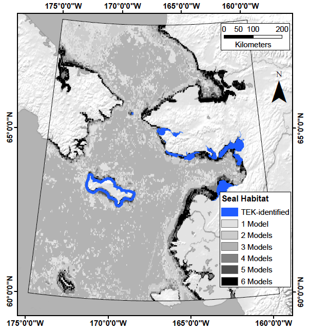
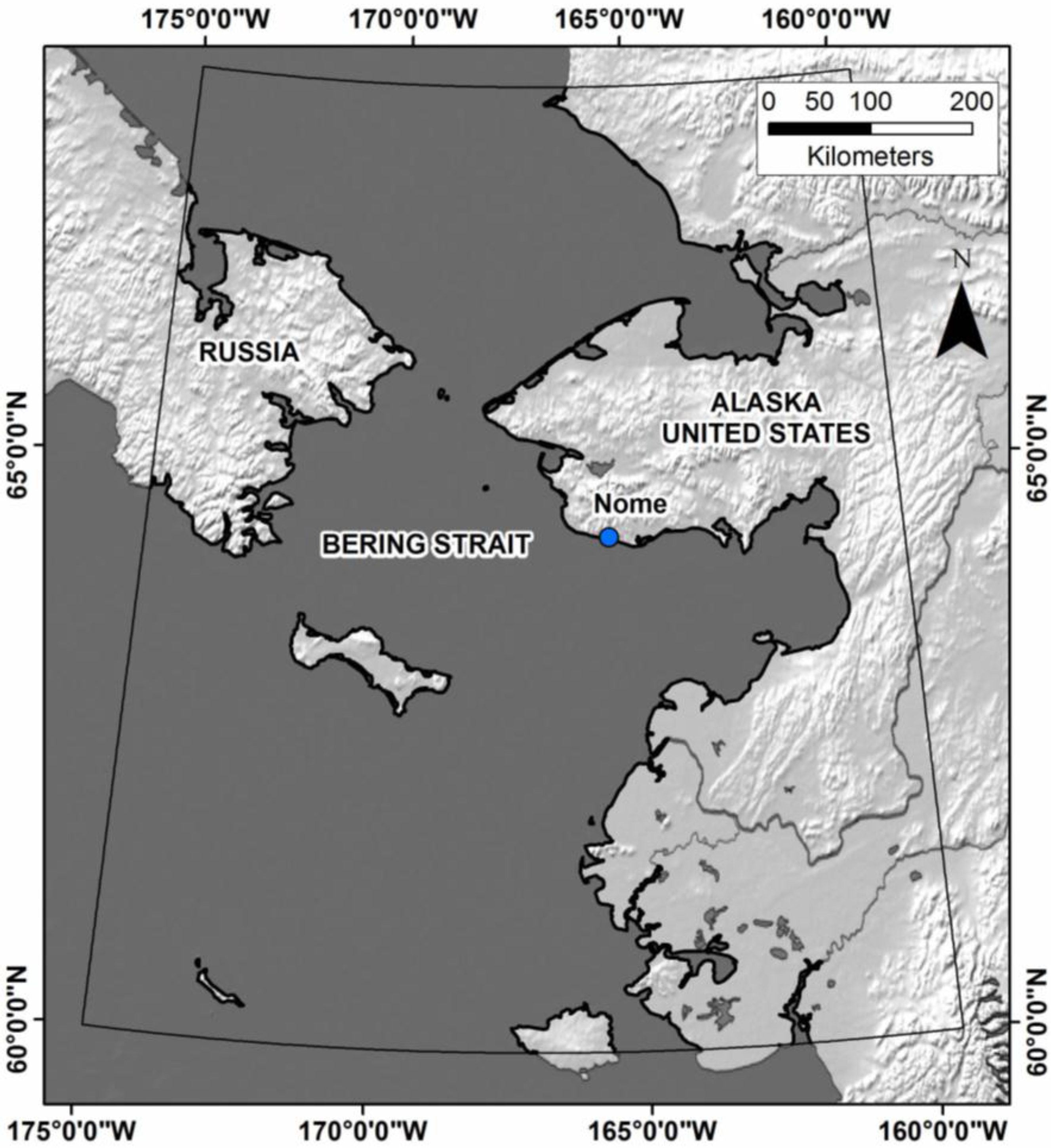
2.1. Study Area

2.2. Predictor Variables

| Environmental Data (Predictor Variables) | Temporal Range | Native Spatial Resolution | Data Source |
|---|---|---|---|
| Bathymetry (m) | N/A | 0.833 km | SRTM30_Plus |
| Bathymetric slope (degrees) | N/A | 4.167 km | SRTM30_Plus |
| Distance from coast (km) | N/A | N/A | Alaska Geospatial Clearinghouse |
| Distance from anadromous streams (km) | N/A | N/A | Alaska Geospatial Clearinghouse |
| Chlorophyll-a concentration (mg∙m3) | 2003–2012 | 4.167 km | NASA Ocean Biology Processing Group |
| Instantaneous Photosynthetically Available Radiation (Einstein m2∙sec) | 2003–2012 | 4.167 km | NASA Ocean Biology Processing Group |
| Photosynthetically Available Radiation (Einstein m2∙Day) | 2003–2012 | 4.167 km | NASA Ocean Biology Processing Group |
| Suspended solids (mol∙M3) | 2003–2012 | 4.167 km | NASA Ocean Biology Processing Group |
| Sea surface temperature (degrees Celsius) | 2003–2012 | 4.167 km | NASA Ocean Biology Processing Group |
| Sea ice (presence) | 2003–2012 | 3.607 km | NASA National Snow and Ice Data Center |
| Reflectance: Band 1 (R) | 2003–2012 | 0.986 km | NASA Land Products Group |
| Reflectance: Band 3 (B) | 2003–2012 | 0.986 km | NASA Land Products Group |
| Reflectance: Band 4 (G) | 2003–2012 | 0.986 km | NASA Land Products Group |
2.3. Remotely-Sensed Data
2.4. Other Spatial Data
2.5. Response Variables

2.6. Data Extent and Pre-Processing
| Raster Layer Name | TS | TS-SD | TS-SD-SB | NTS | NTS-SD | NTS-SD-SB | Input Band |
|---|---|---|---|---|---|---|---|
| B01 TS Intercept | + | + | + | − | − | − | 1 |
| B01 TS Slope | + | + | + | − | − | − | 2 |
| B03 TS Intercept | + | + | + | − | − | − | 3 |
| B03 TS Slope | + | + | + | − | − | − | 4 |
| B04 TS Intercept | + | + | + | − | − | − | 5 |
| B04 TS Slope | + | + | + | − | − | − | 6 |
| Chlorophyll-a TS Intercept | + | + | + | − | − | − | 9 |
| Chlorophyll-a TS Slope | + | + | + | − | − | − | 10 |
| IPAR TS Intercept | + | + | + | − | − | − | 14 |
| IPAR TS Slope | + | + | + | − | − | − | 15 |
| PAR TS Intercept | + | + | + | − | − | − | 17 |
| PAR TS Slope | + | + | + | − | − | − | 18 |
| Sea Ice TS Intercept | + | + | + | − | − | − | 20 |
| Sea Ice TS Slope | + | + | + | − | − | − | 21 |
| Suspended Solids TS Intercept | + | + | + | − | − | − | 22 |
| Suspended Solids TS Slope | + | + | + | − | − | − | 23 |
| Sea Surface Temperature TS Intercept | + | + | + | − | − | − | 25 |
| Sea Surface Temperature TS Slope | + | + | + | − | − | − | 26 |
| Bathymetry Depth | + | + | − | + | + | − | 7 |
| Bathymetry Slope | + | + | − | + | + | − | 8 |
| Distance from Stream Outlets | + | − | − | + | − | − | 12 |
| Distance from Coast | + | − | − | + | − | − | 13 |
| Chlorophyll OC Climatology | + | + | + | + | + | + | 11 |
| IPAR OC Climatology | + | + | + | + | + | + | 16 |
| PAR OC Climatology | + | + | + | + | + | + | 19 |
| Suspended Solids OC Climatology | + | + | + | + | + | + | 24 |
| Sea Surface Temperature OC Climatology | + | + | + | + | + | + | 27 |
2.7. Analysis
3. Results
3.1. What Is the Optimal Number of Training and Validation Points to Use in a Classification?
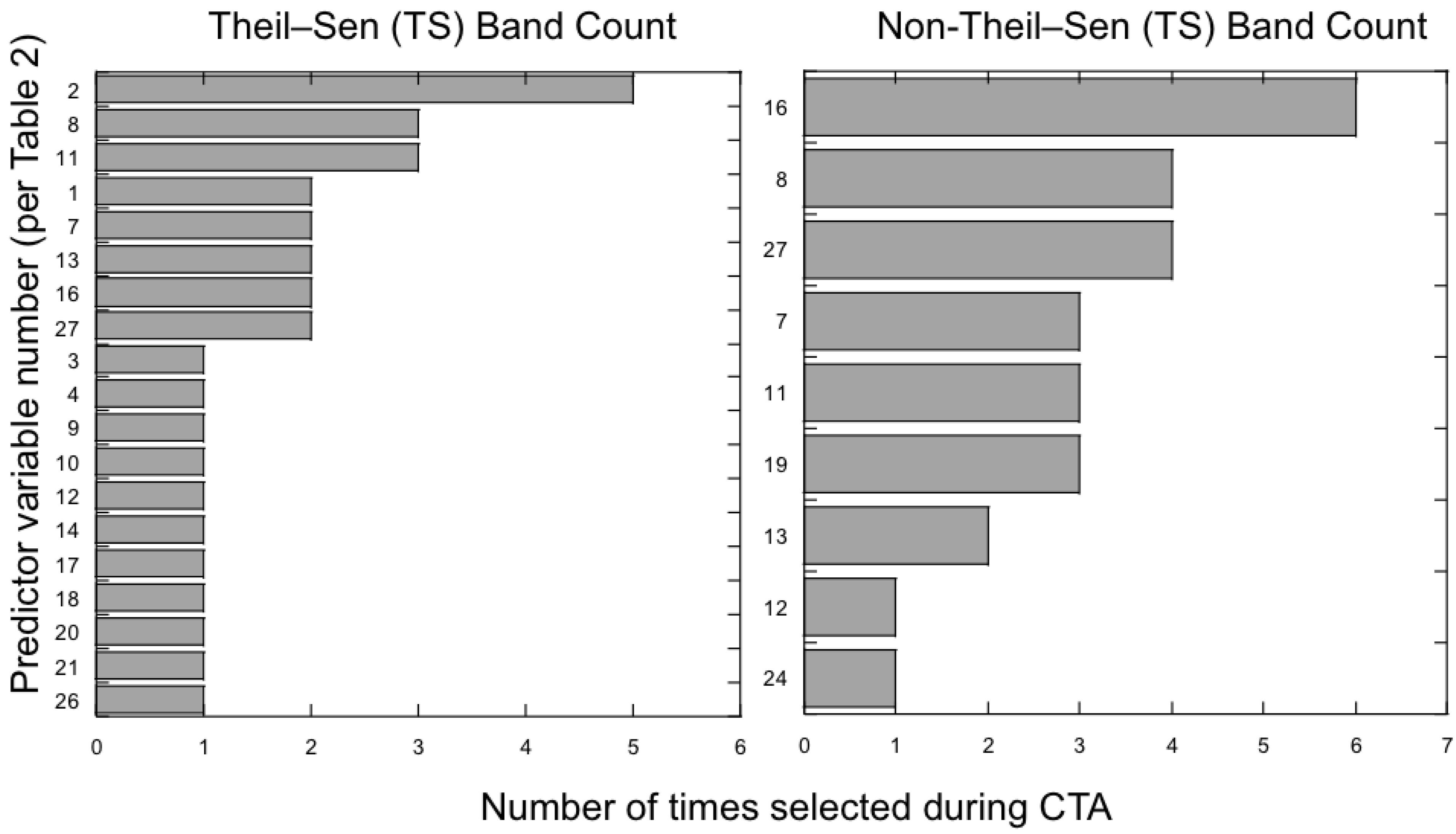
3.2. Which Predictor Variables Provide the Most Useful Information for Classification?


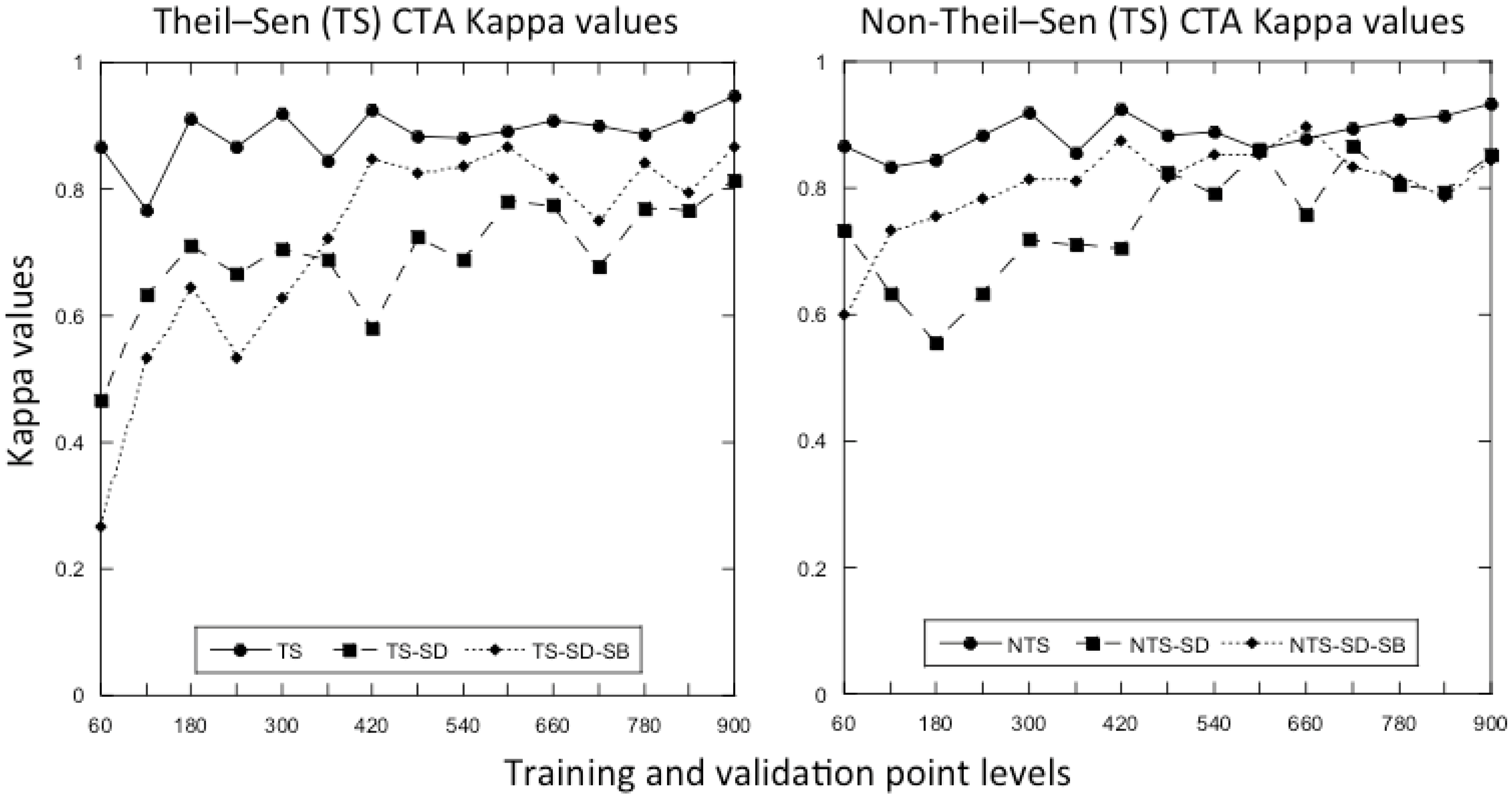
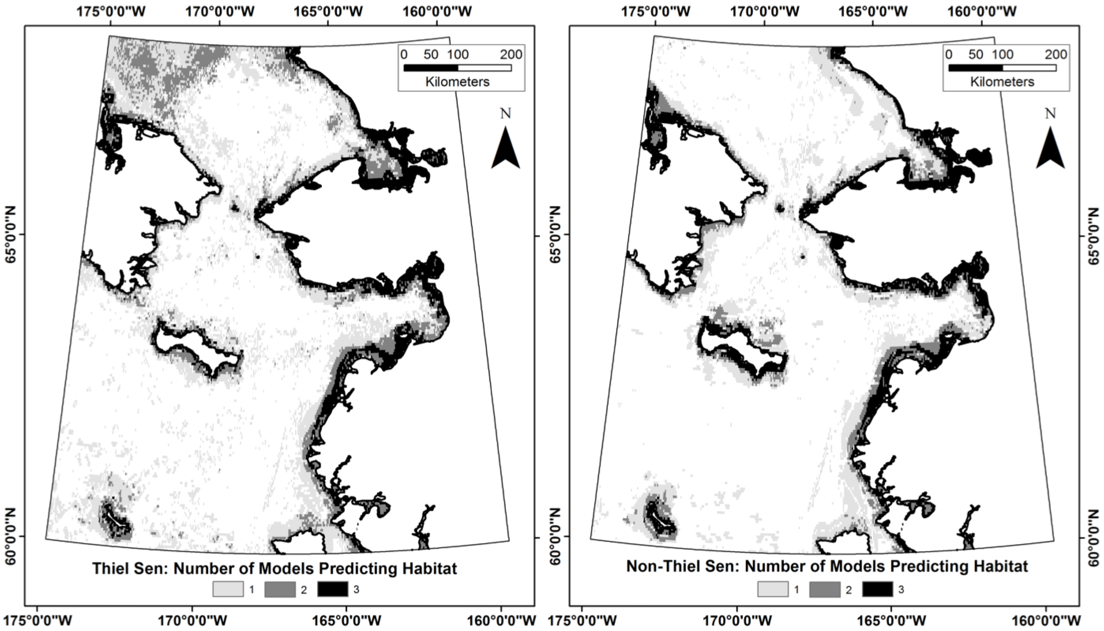
3.3. Does the Theil–Sen Time Series Data Improve the Accuracy of the Classification?


| TS | TS-SD | TS-SD-SB | NTS | NTS-SD | NTS-SD-SB | |
|---|---|---|---|---|---|---|
| Band Count | 7 | 15 | 10 | 6 | 12 | 9 |
| Cells Selected | 8176 | 11,939 | 11,525 | 7909 | 8421 | 8403 |
| Kappa | 0.883 | 0.725 | 0.825 | 0.883 | 0.825 | 0.817 |
4. Discussion
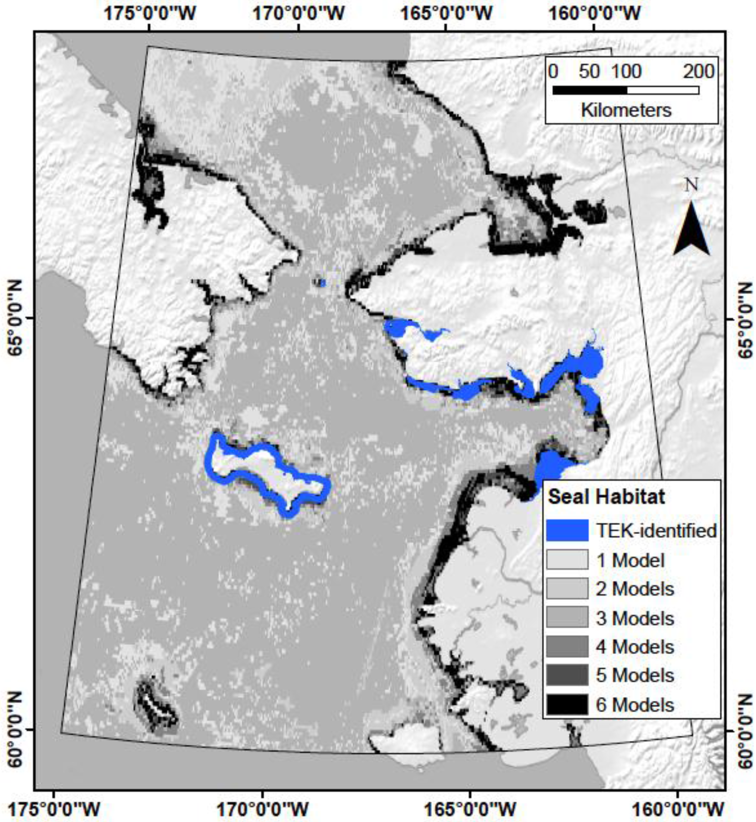
4.1. Does TEK Function as a Reasonable Proxy for Western Scientific Data?
4.2. What Is the Optimal Number of Training and Validation Points to Use in a Classification?
4.3. Which Predictor Variables Provide the Most Information for Classification?
4.4. Is the Time Series Data Useful for the Classification Analysis?
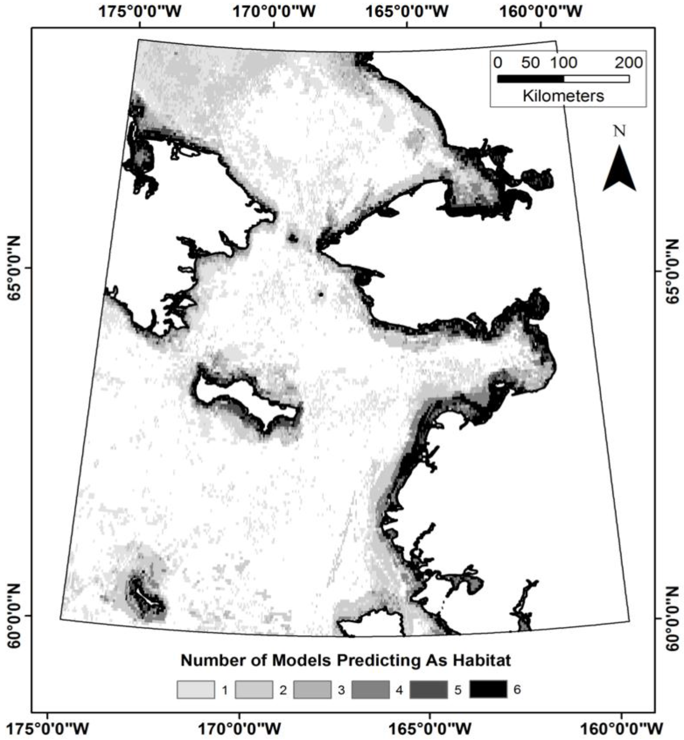
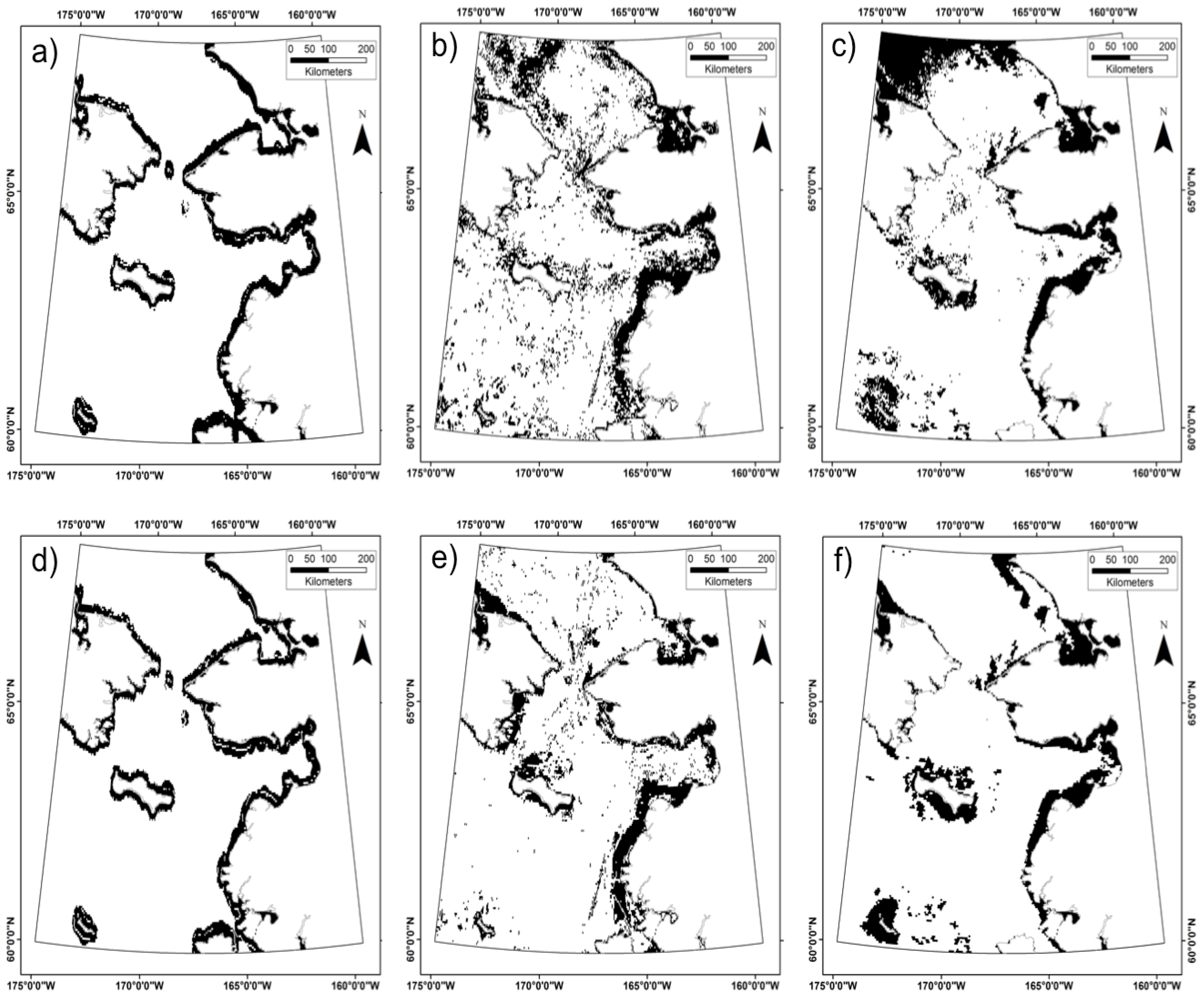
4.5. What Are the Utilities, Applications, and Limitations of the Model?
5. Conclusions
Acknowledgments
Author Contributions
Conflicts of Interest
References
- Ackerman, R.E. Early maritime traditions in the Bering, Chukchi, and east Siberian seas. Arct. Anthropol. 1998, 35, 247–262. [Google Scholar]
- Gadamus, L. Linkages between human health and ocean health: A participatory climate change vulnerability assessment for marine mammal harvesters. Int. J. Circumpolar Health 2013, 72, 20715. [Google Scholar] [CrossRef] [PubMed] [Green Version]
- Ahmasuk, A.; Trigg, E.; Magdanz, J.; Robbins, B. A Comprehensive Subsistence Use Study of the Bering Strait Region; Kawerak, Inc.: Nome, AK, USA, 2008. [Google Scholar]
- Moore, S.E.; Huntington, H.P. Arctic marine mammals and climate change: Impacts and resilience. Ecol. Appl. 2008, 18, S157–S165. [Google Scholar] [CrossRef] [PubMed]
- Grebmeier, J.M. Shifting patterns of life in the pacific arctic and sub-arctic seas. Annu. Rev. Mar. Sci. 2012, 4, 63–78. [Google Scholar] [CrossRef] [PubMed]
- Laidre, K.L.; Stirling, I.; Lowry, L.F.; Wiig, O.; Heide-Jorgensen, M.P.; Ferguson, S.H. Quantifying the sensitivity of arctic marine mammals to climate-induced habitat change. Ecol. Appl. 2008, 18, S97–S125. [Google Scholar] [CrossRef] [PubMed]
- Burek, A.; Gulland, F.M.D.; O’Hara, T.M. Effects of climate change on arctic marine mammal health. Ecol. Appl. 2008, 18, S126–S134. [Google Scholar] [CrossRef] [PubMed]
- Stafford, K. Anthropogenic Sound and Marine Mammals in the Arctic; The Pew Charitable Trusts: Seattle, WA, USA, 2013. [Google Scholar]
- Sackinger, W.M.; Jeffries, M.O. Symposium on noise and marine mammals. In Port and Ocean Engineering under Arctic Conditions; Sackinger, W.M., Jeffries, M.O., Eds.; The Geophysical Institute, University of Alaska Fairbanks: Anchorage, AK, USA, 1988; p. 131. [Google Scholar]
- Huntington, H.P. A preliminary assessment of threats to arctic marine mammals and their conservation in the coming decades. Mar. Policy 2009, 33, 77–82. [Google Scholar] [CrossRef]
- Maslowski, W.; Kinney, J.C.; Higgins, M.; Roberts, A. The future of arctic sea ice. Annu. Rev. Earth Planet. Sci. 2012, 40, 625–654. [Google Scholar] [CrossRef]
- Kwok, R.; Untersteiner, N. The thinning of arctic sea ice. Phys. Today 2011, 64, 36–41. [Google Scholar] [CrossRef]
- Douglas, D.C. Arctic Sea Ice Decline: Projected Changes in Timing and Extent of Sea Ice in the Bering and Chukchi Seas; U.S. Geological Survey: Reston, VA, USA, 2010. [Google Scholar]
- Walsh, J.E.; Overland, J.E.; Groisman, P.Y.; Rudolf, B. Ongoing climate change in the arctic. AMBIO 2011, 40, 6–16. [Google Scholar] [CrossRef]
- Kwok, R.; Rothrock, D.A. Decline in arctic sea ice thickness from submarine and icesat records: 1958–2008. Geophys. Res. Lett. 2009, 36, L15501. [Google Scholar] [CrossRef]
- Wang, M.; Overland, J.E.; Stabeno, P. Future climate of the Bering and Chukchi seas projected by global climate models. Deep Sea Res. II: Top. Stud. Oceanogr. 2012, 65–70, 46–57. [Google Scholar] [CrossRef]
- Arctic Council. Arctic Marine Shipping Assessment 2009 Report, 2nd ed.; Arctic Council: Tromsø, Norway, 2009. [Google Scholar]
- Brigham, L.; Smith, E. The Future of Arctic Marine Navigation in Mid-Century; Arctic Council: Tromsø, Norway, 2008. [Google Scholar]
- Kitagawa, H. Arctic routing: Challenges and opportunities. WMU J. Marit. Aff. 2008, 7, 485–503. [Google Scholar] [CrossRef]
- Stephenson, S.R.; Smith, L.C.; Brigham, L.W.; Agnew, J.A. Projected 21st-century changes to arctic marine access. Clim. Chang. 2013, 118, 885–899. [Google Scholar] [CrossRef]
- Conley, H.; Pumphrey, D.L. Arctic Economics in the 21st Century: The Benefits and Costs of Cold; Center for Strategic & International Studies: Washington, DC, USA, 2013. [Google Scholar]
- Wolfe, R.J.; Walker, R.J. Subsistence economies in Alaska: Productivity, geography, and development impacts. Arct. Anthropol. 1987, 24, 56–81. [Google Scholar]
- Ackerman, R.E. Settlements and sea mammal hunting in the Bering-Chukchi sea region. Arct. Anthropol. 1988, 25, 52–79. [Google Scholar]
- Huntington, H.P.; Sookiayak, C. Traditional Ecological Knowledge of Seals in Norton Bay, Alaska; Elim-Shaktoolik-Koyuk Marine Mammal Commission: Eagle River, AK, USA, 2000. [Google Scholar]
- Katsanevakis, S.; Stelzenmuller, V.; South, A.; Sorensen, T.K.; Jones, P.J.S.; Kerr, S.; Badalamenti, F.; Anagnostou, C.; Breen, P.; Chust, G.; et al. Ecosystem-based marine spatial management: Review of concepts, policies, tools, and critical issues. Ocean. Coast. Manag. 2011, 54, 807–820. [Google Scholar] [CrossRef]
- Kaplan, D.M.; Planes, S.; Fauvelot, C.; Brochier, T.; Lett, C.; Bodin, N.; Le Loc’h, F.; Tremblay, Y.; Georges, J.-Y. New tools for the spatial management of living marine resources. Curr. Opin. Environ. Sustain. 2010, 2, 88–93. [Google Scholar] [CrossRef]
- Wilson, C.D.; Roberts, D.; Reid, N. Applying species distribution modelling to identify areas of high conservation value for endangered species: A case study using Margaritifera margaritifera (L.). Biol. Conserv. 2011, 144, 821–829. [Google Scholar] [CrossRef]
- Schofield, G.; Scott, R.; Dimadi, A.; Fossette, S.; Katselidis, K.A.; Koutsoubas, D.; Lilley, M.K.S.; Pantis, J.D.; Karagouni, A.D.; Hays, G.C. Evidence-based marine protected area planning for a highly mobile endangered marine vertebrate. Biol. Conserv. 2013, 161, 101–109. [Google Scholar] [CrossRef]
- Schmelzer, I. Seals and seascapes: Covariation in Hawaiian monk seal subpopulations and the oceanic landscape of the Hawaiian archipelago. J. Biogeogr. 2000, 27, 901–914. [Google Scholar] [CrossRef]
- Boyd, D.S.; Foody, G.M. An overview of recent remote sensing and GIS-based research in ecological informatics. Ecol. Inform. 2011, 6, 25–36. [Google Scholar] [CrossRef]
- Guisan, A.; Zimmermann, N. Predictive habitat distribution models in ecology. Ecol. Model. 2000, 135, 147–186. [Google Scholar] [CrossRef]
- Elith, J.; Leathwick, J.R. Species distribution models: Ecological explanation and prediction across space and time. Annu. Rev. Ecol. Evol. Syst. 2009, 40, 677–697. [Google Scholar] [CrossRef]
- Guisan, A.; Thuiller, W. Predicting species distribution: Offering more than simple habitat models. Ecol. Lett. 2005, 8, 993–1009. [Google Scholar] [CrossRef]
- Miller, J. Species distribution modeling. Geogr. Compass 2010, 4, 490–509. [Google Scholar] [CrossRef]
- Dobrowski, S.Z.; Safford, H.D.; Cheng, Y.B.; Ustin, S.L. Mapping mountain vegetation using species distribution modeling, image-based texture analysis, and object-based classification. Appl. Veg. Sci. 2008, 11, 499–508. [Google Scholar] [CrossRef]
- Treitz, P.; Howarth, P. Integrating spectral, spatial, and terrain variables for forest ecosystem classification. Photogramm. Eng. Remote Sens. 2000, 66, 305–317. [Google Scholar]
- Vogelmann, J.E.; Sohl, T.; Howard, S.M. Regional characterization of land cover using multiple sources of data. Photogramm. Eng. Remote Sens. 1998, 64, 45–57. [Google Scholar]
- Mumby, P.; Green, E.; Edwards, A.; Clark, C. Coral reef habitat mapping: How much detail can remote sensing provide? Mar. Biol. 1997, 130, 193–202. [Google Scholar] [CrossRef]
- Kachelriess, D.; Wegmann, M.; Gollock, M.; Pettorelli, N. The application of remote sensing for marine protected area management. Ecol. Indic. 2014, 36, 169–177. [Google Scholar] [CrossRef]
- Azzellino, A.; Panigada, S.; Landredi, C.; Zanardelli, M.; Airoldi, S.; Notarbartolo di Sciara, G. Predictive habitat models for managing marine areas: Spatial and temporal distribution of marine mammals within the Pelagos sanctuary (northwestern Mediterranean sea). Ocean. Coast. Manag. 2012, 67, 63–74. [Google Scholar] [CrossRef]
- Polovina, J.; Howell, E.; Kobayashi, D.; Seki, M. The transition zone chlorophyll front, a dynamic global feature defining migration and forage habitat for marine resources. Prog. Oceanogr. 2001, 49, 461–483. [Google Scholar] [CrossRef]
- Mishra, D.; Narumalani, S.; Rundquist, D.; Lawson, M. Benthic habitat mapping in tropical marine environments using Quickbird multispectral data. Photogramm. Eng. Remote Sens. 2006, 72, 1037–1048. [Google Scholar] [CrossRef]
- Alaska Department of Fish and Game. Ice Seal Movement and Habitat Use Study. Available online: http://www.adfg.alaska.gov/index.cfm?adfg=marinemammalprogram.icesealmovements (accessed on 10 August 2015).
- Kawerak Inc. Traditions of Respect: Traditional Knowledge from Kawerak’s Ice Seal and Walrus Project; Kawerak Social Science Program: Nome, AK, USA, 2013. [Google Scholar]
- Kawerak Inc. Seal and Walrus Harvest and Habitat Areas for Nine Bering Strait Region Communities; Kawerak Social Science Program: Nome, AK, USA, 2013. [Google Scholar]
- National Marine Fisheries Service (NMFS). Endangered and Threatened Species; Threatened Status for the Beringia and Okhotsk Distinct Population Segments of the Erignathus Barbatus Nauticus Subspecies of the Bearded Seal; NMFS: Washington, DC, USA, 2012; Volume 77, pp. 76740–76768. [Google Scholar]
- Burns, J.J. Bearded seal—Erignathus barbatus. In Handbook of Marine Mammals; Ridgway, S.H., Harrison, R.J., Eds.; Academic Press, Inc.: New York, NY, USA, 1981; Volume 2, pp. 145–170. [Google Scholar]
- Quakenbush, L.; Citta, J.; Crawford, J. Biology of the Bearded Seal (Erignathus barbatus) in Alaska, 1961–2009; Arctic Marine Mammal Program: Fairbanks, AK, USA, 2011; p. 71. [Google Scholar]
- Cameron, M.F.; Bengston, J.L.; Boveng, P.L.; Jansen, J.K.; Kelly, B.P.; Dahle, S.P.; Logerwell, E.A.; Overland, J.E.; Sabine, C.L.; Waring, G.T.; et al. Status Review of the Bearded Seal (Erignathus barbatus); U.S. Department of Commerce: Washington, DC, USA, 2010. [Google Scholar]
- National Marine Fisheries Service (NMFS). Bearded Seal Range; Office of Protected Resources-NMFS: Silver Spring, MD, USA, 2009. [Google Scholar]
- Ver Hoef, J.M.; Cameron, M.F.; Boveng, P.L.; London, J.M.; Moreland, E.E. A spatial hierarchical model for abundance of three ice-associated seal species in the eastern Bering sea. Stat. Methodol. 2014, 17, 46–66. [Google Scholar] [CrossRef]
- Berkes, F.; Colding, J.; Folke, C. Rediscovery of traditional ecological knowledge as adaptive management. Ecol. Appl. 2000, 10, 1251–1262. [Google Scholar] [CrossRef]
- Giddings, J.L. Cultural continuities of Eskimos. Am. Antiq. 1961, 27, 155–173. [Google Scholar] [CrossRef]
- Dumond, D.E. The norton tradition. Arct. Anthropol. 2000, 37, 1–22. [Google Scholar]
- Strahler, A.H.; Woodcock, C.E.; Smith, J.A. On the nature of models in remote sensing. Remote Sens. Environ. 1986, 20, 121–139. [Google Scholar] [CrossRef]
- Woodcock, C.E.; Strahler, A.H. The factor of scale in remote sensing. Remote Sens. Environ. 1987, 21, 311–332. [Google Scholar] [CrossRef]
- Pease, C.H.; Schoenberg, S.A.; Overland, J.E. A Climatology of the Bering Sea and Its Relation to the Sea Ice Extent; Pacific Marine Environmental Laboratory: Seattle, WA, USA, 1982. [Google Scholar]
- Loughlin, T.R.; Sukhanova, I.N.; Sinclair, E.H.; Ferrero, R.C. Summary of biology and ecosystem dynamics in the Bering sea. In Ak-sg-99–03: Dynamics of the Bering Sea; Loughlin, T.R., Ohtani, K., Eds.; University of Alaska Sea Grant, North Pacific Marine Science Organization (PICES): Fairbanks, AK, USA, 1999; pp. 387–407. [Google Scholar]
- Pittman, S.J.; Costa, B. Linking cetaceans to their environment: Spatial data acquisition, digital processing and predictive modeling for marine spatial planning in the Northwest Atlantic. In Spatial Complexity, Informatics, and Wildlife Conservation; Cushman, S.A., Huettmann, F., Eds.; Springer: New York, NY, USA, 2010; pp. 387–408. [Google Scholar]
- Phinn, S.R. A framework for selecting appropriate remotely sensed data dimensions for environmental monitoring and management. Int. J. Remote Sens. 1998, 19, 3457–3463. [Google Scholar] [CrossRef]
- Phinn, S.R.; Stow, D.A.; Franklin, J.; Mertes, L.A.K.; Michaelsen, J. Remotely sensed data for ecosystem analyses: Combining hierarchy theory and scene models. Environ. Manag. 2003, 31, 429–441. [Google Scholar] [CrossRef] [PubMed]
- NASA. MODIS Overview. Available online: https://lpdaac.usgs.gov/products/modis_overview (accessed on 15 August 2015).
- State of Alaska. Alaska State Geo-Spatial Data Clearinghouse. Available online: http://www.asgdc.state.ak.us/ (accessed on 12 April 2013).
- Becker, J.J.; Sandwell, D.T.; Smith, W.H.F.; Braud, J.; Binder, B.; Depner, J.; Fabre, D.; Factor, J.; Ingalls, S.; Kim, S.-H.; et al. Global bathymetry and elevation data at 30 arc seconds resolution: Srtm30_plus. Mar. Geod. 2009, 32, 355–371. [Google Scholar] [CrossRef]
- Brotons, L.; Thuiller, W.; Araujo, M.B.; Hirzel, A.H. Presence-absence versus presence-only modelling methods for predicting bird habitat suitability. Ecography 2004, 27, 437–448. [Google Scholar] [CrossRef]
- Hirzel, A.H.; Le Lay, G.; Helfer, V.; Randin, C.; Guisan, A. Evaluating the ability of habitat suitability models to predict species presences. Ecol. Modell. 2006, 199, 142–152. [Google Scholar] [CrossRef]
- Sequeira, A.; Mellin, C.; Rowat, D.; Meekan, M.G.; Bradshaw, C.J.A. Ocean-scale prediction of whale shark distribution. Divers. Distrib. 2012, 18, 504–518. [Google Scholar] [CrossRef]
- Wisz, M.S.; Guisan, A. Do pseudo-absence selection strategies influence species distribution models and their predictions? An information-theoretic approach based on simulated data. BMC Ecol. 2009, 9, 8. [Google Scholar] [CrossRef] [PubMed]
- Stokland, J.N.; Halvorsen, R.; Stoa, B. Species distribution modelling—Effect of design and sample size of pseudo-absence observations. Ecol. Modell. 2011, 222, 1800–1809. [Google Scholar] [CrossRef]
- Fenna, D. Cartographic Science: A Compendium of Map Projections, with Derivations; CRC Press: Boca Raton, FL, USA, 2007. [Google Scholar]
- Snyder, J.P. Flattening the Earth: Two Thousand Years of Map Projections; The University of Chicago Press: Chicago, IL, USA, 1993. [Google Scholar]
- Eastman, J.R.; Sangermano, F.; Ghimire, B.; Zhu, H.; Chen, H.; Neeti, N.; Cai, Y.; Machado, E.A.; Crema, S.C. Seasonal trend analysis of image time series. Int. J. Remote Sens. 2009, 30, 2721–2726. [Google Scholar] [CrossRef]
- Neeti, N.; Eastman, J.R. A contextual Mann-Kendall approach for the assessment of trend significance in image time series. Trans. GIS 2011, 15, 599–611. [Google Scholar] [CrossRef]
- Fernandes, R.; Leblanc, S.G. Parametric (modified least squares) and non-parametric (Theil–Sen) linear regressions for predicting biophysical parameters in the presence of measurement errors. Remote Sens. Environ. 2005, 95, 303–316. [Google Scholar] [CrossRef]
- Eastman, J.R.; Sangermano, F.; Machado, E.A.; Rogan, J.; Anyamba, A. Global trends in seasonality of normalized difference vegetation index (NDVI), 1982–2011. Remote Sens. 2013, 5, 4799–4818. [Google Scholar] [CrossRef]
- Campbell, J.W.; Blaisdell, J.M.; Darzi, M. SeaWiFS Data Products: Spatial and Temporal Binning Algorithms; SeaWiFS Technical Report Series; Goddard Space Flight Center: Greenbelt, MD, USA, 1995. [Google Scholar]
- Austin, M.P. Spatial prediction of species distribution: An interface between ecological theory and statistical modelling. Ecol. Modell. 2002, 157, 101–118. [Google Scholar] [CrossRef]
- Miller, J.; Franklin, J. Modeling the distribution of four vegetation alliances using generalized linear models and classification trees with spatial dependence. Ecol. Modell. 2002, 157, 227–247. [Google Scholar] [CrossRef]
- De’Ath, G.; Fabribius, K.E. Classification and regression trees: A powerful yet simple technique for ecological data analysis. Ecology 2000, 81, 3178–3192. [Google Scholar] [CrossRef]
- Loh, W.-Y. Classification and regression trees. WIREs Data Min. Knowl. Discov. 2011, 1, 14–23. [Google Scholar] [CrossRef]
- Zambon, M.; Lawrence, R.; Bunn, A.; Powell, S. Effect of alternative splitting rules on image processing using classification tree analysis. Photogramm. Eng. Remote Sens. 2006, 72, 25–30. [Google Scholar] [CrossRef]
- Lawrence, R.L.; Wright, A. Rule-based classification systems using classification and regression tree (CART) analysis. Photogramm. Eng. Remote Sens. 2001, 67, 1137–1142. [Google Scholar]
- Qiu, F.; Jensen, J.R. Opening the black box of neural networks for remote sensing image classification. Int. J. Remote Sens. 2004, 25, 1749–1768. [Google Scholar] [CrossRef]
- Congalton, R.G. Accuracy assessment and validation of remotely sensed and other spatial information. Int. J. Wildland Fire 2001, 10, 321–328. [Google Scholar] [CrossRef]
- Congalton, R.G.; Green, K. Assessing the Accuracy of Remotely Sensed Data: Principles and Practices, 2nd ed.; CRC Press: Boca Raton, FL, USA, 2009. [Google Scholar]
© 2015 by the authors; licensee MDPI, Basel, Switzerland. This article is an open access article distributed under the terms and conditions of the Creative Commons Attribution license (http://creativecommons.org/licenses/by/4.0/).
Share and Cite
Olsen, P.M.; Kolden, C.A.; Gadamus, L. Developing Theoretical Marine Habitat Suitability Models from Remotely-Sensed Data and Traditional Ecological Knowledge. Remote Sens. 2015, 7, 11863-11886. https://doi.org/10.3390/rs70911863
Olsen PM, Kolden CA, Gadamus L. Developing Theoretical Marine Habitat Suitability Models from Remotely-Sensed Data and Traditional Ecological Knowledge. Remote Sensing. 2015; 7(9):11863-11886. https://doi.org/10.3390/rs70911863
Chicago/Turabian StyleOlsen, Patrick M., Crystal A. Kolden, and Lily Gadamus. 2015. "Developing Theoretical Marine Habitat Suitability Models from Remotely-Sensed Data and Traditional Ecological Knowledge" Remote Sensing 7, no. 9: 11863-11886. https://doi.org/10.3390/rs70911863