
Data-Gap Filling to Understand the Dynamic Feedback Pattern of Soil

 ,
, 
Abstract
:
1. Introduction
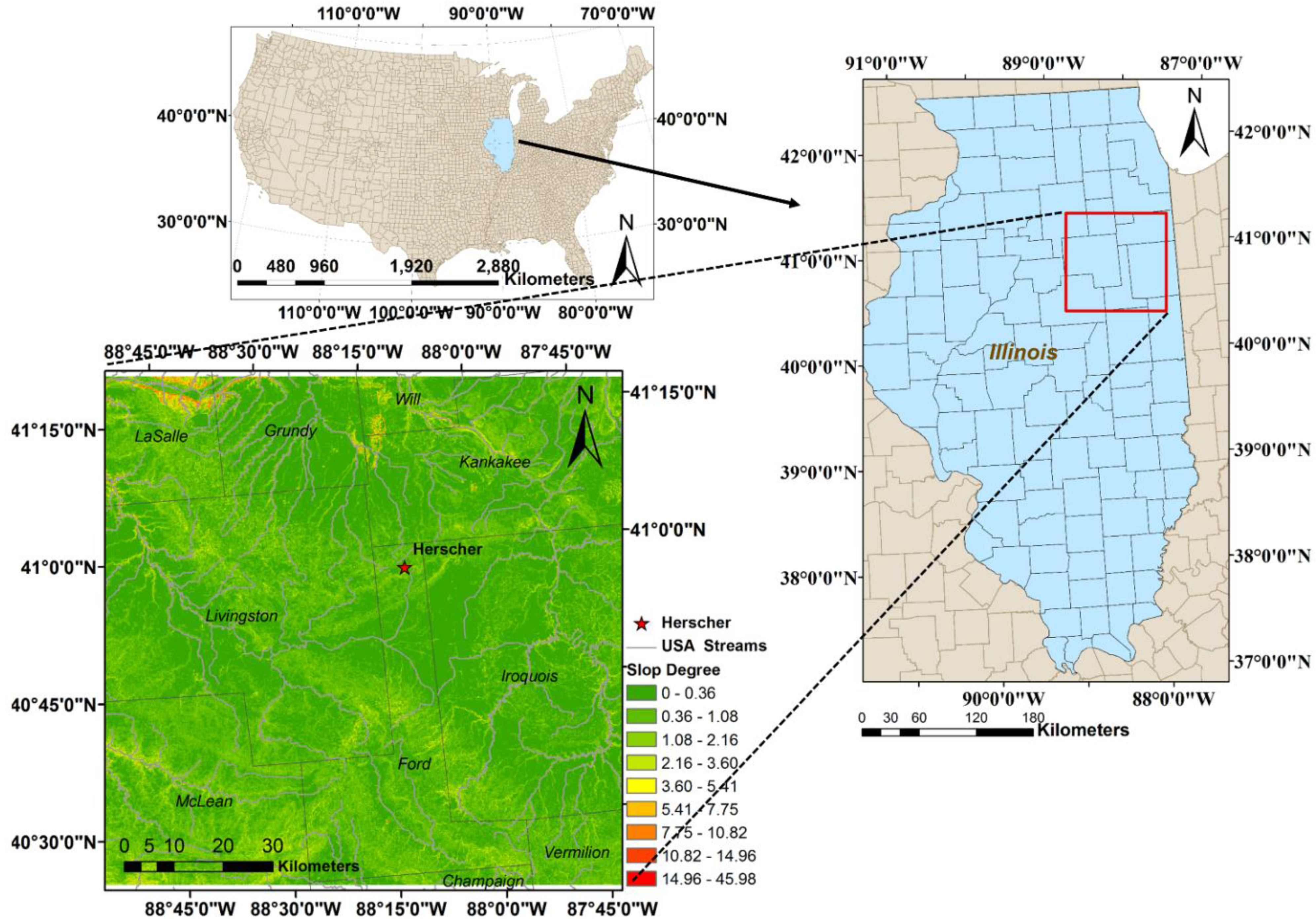
2. Study Area
3. Methodology
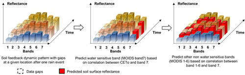
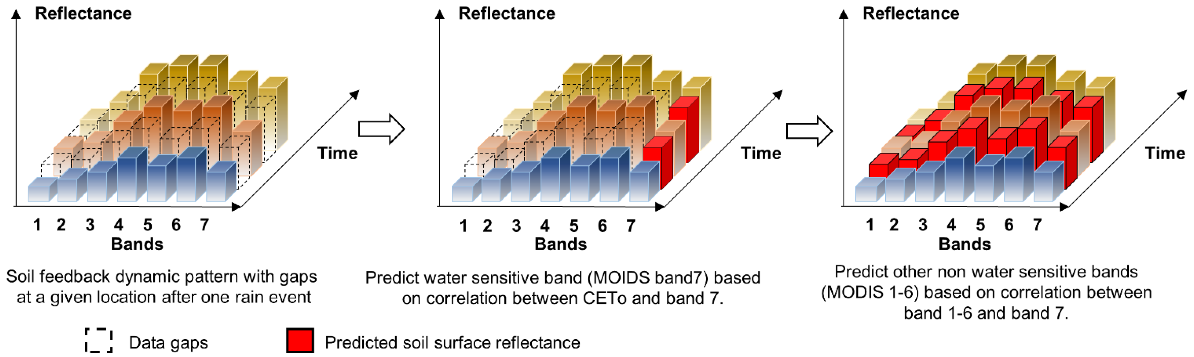
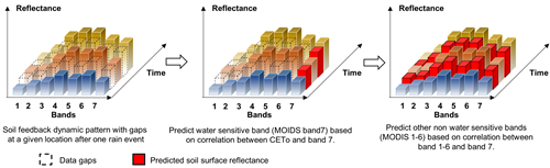
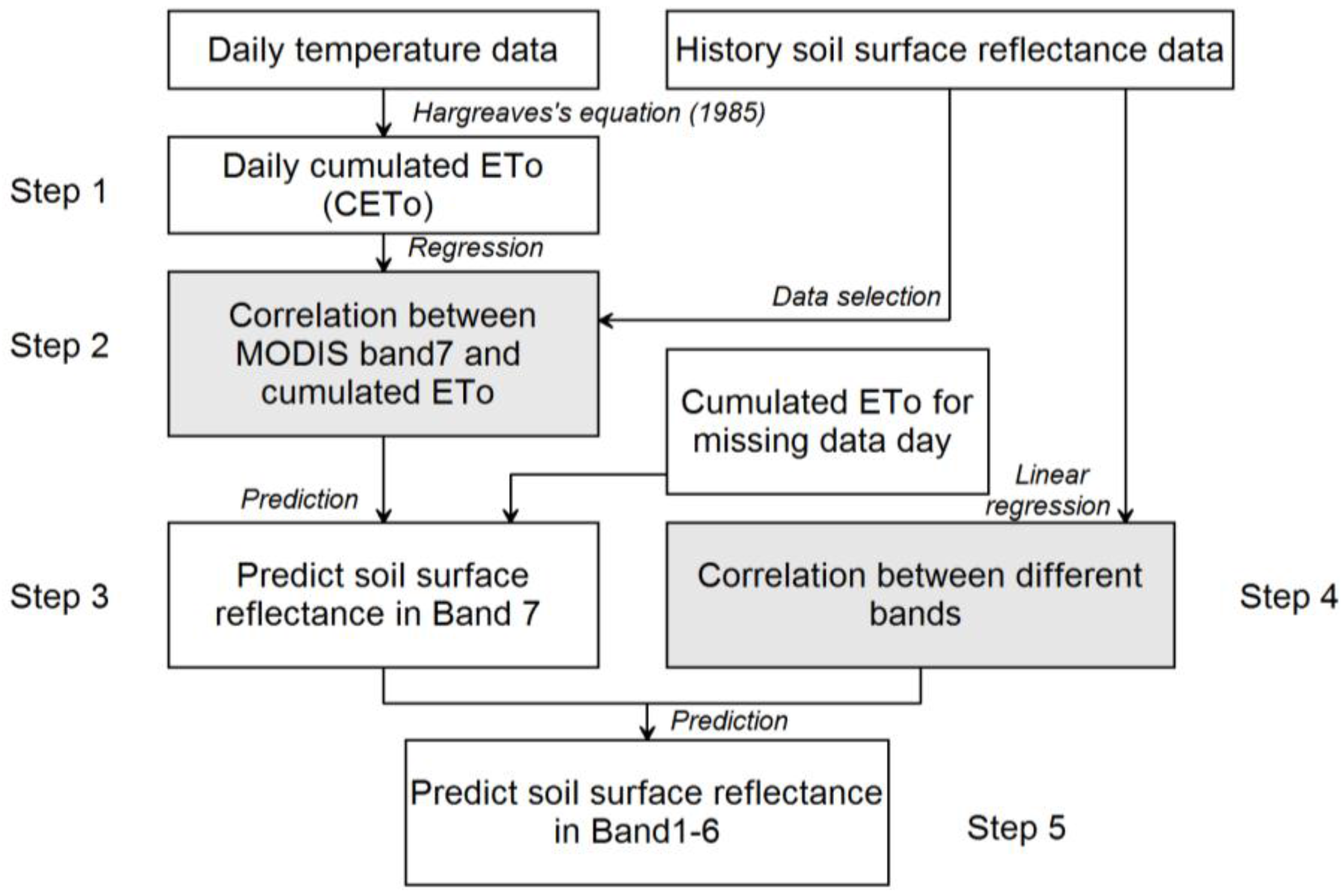
3.1. Basic Concept
3.2. Choosing a Proper Model to Capture Correlation between Soil Surface Reflectance and Evaporation Parameters
3.3. Filling Data Gaps

4. Data Preprocessing and Validation
4.1. Data Collection and Preprocessing
4.2. Validation
5. Results and Discussion
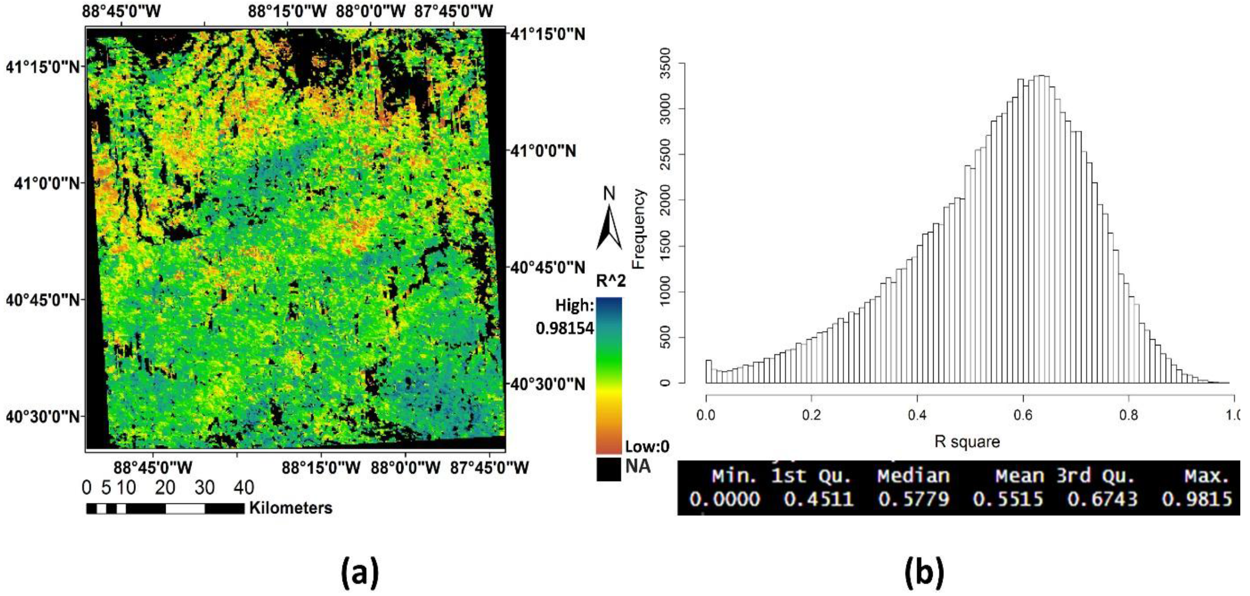
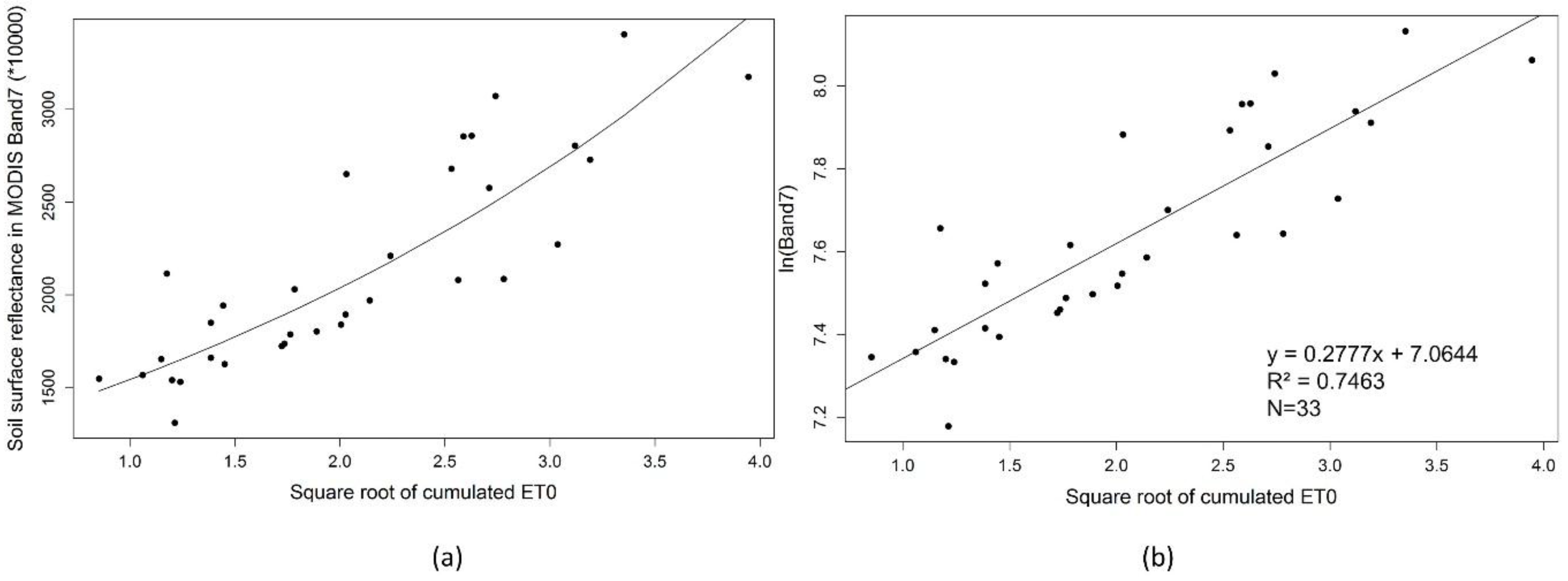
5.1. Correlation between MODIS Band 7 and Cumulative ET0 (CET0)

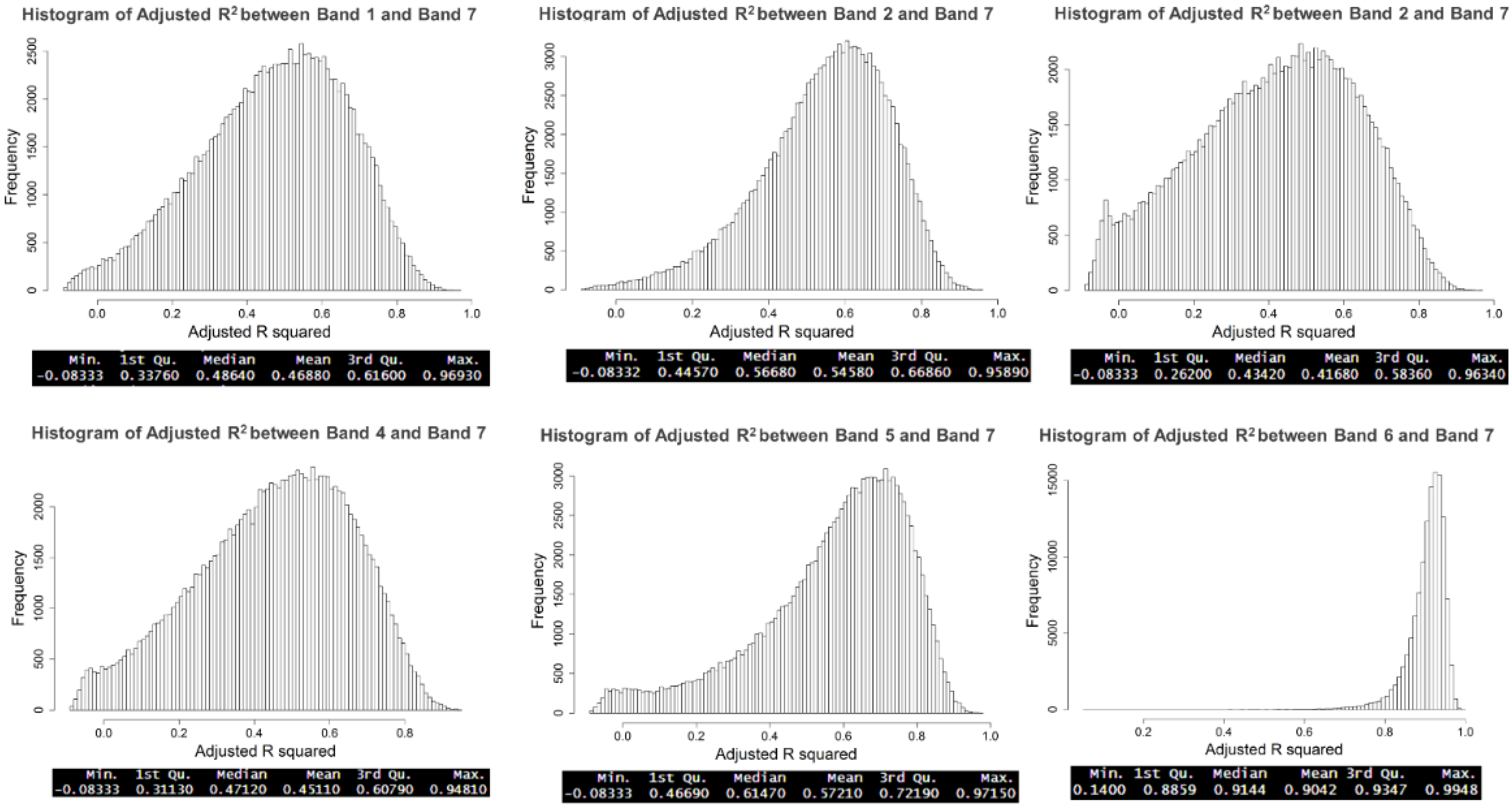
5.2. Correlation among MODIS Bands

| Band 1 | Band 2 | Band 3 | Band 4 | Band 5 | Band 6 | |
|---|---|---|---|---|---|---|
| Band 7 | 0.461 | 0.505 | 0.496 | 0.642 | 0.607 | 0.915 |

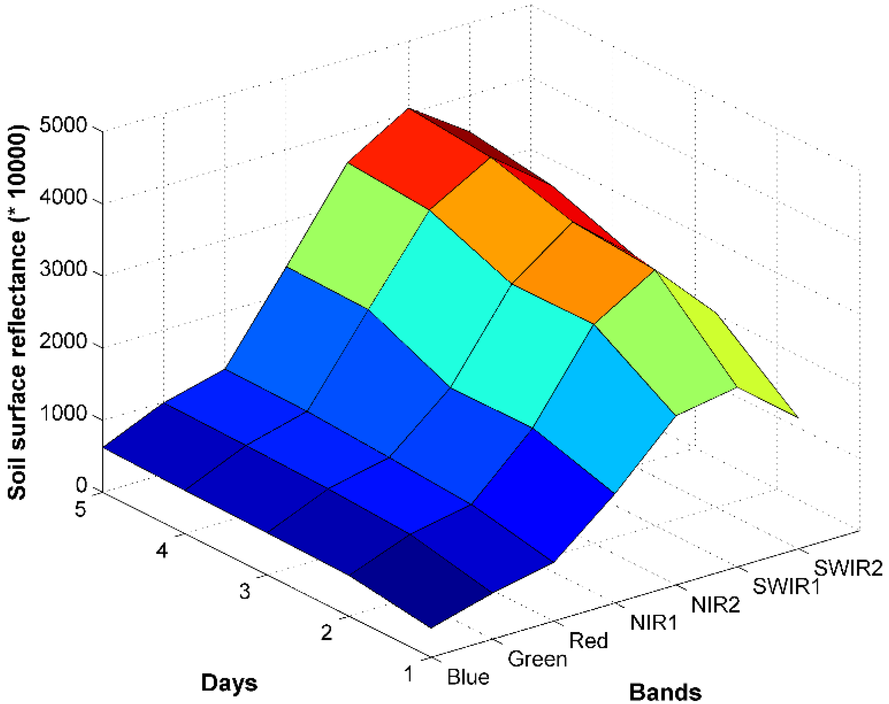
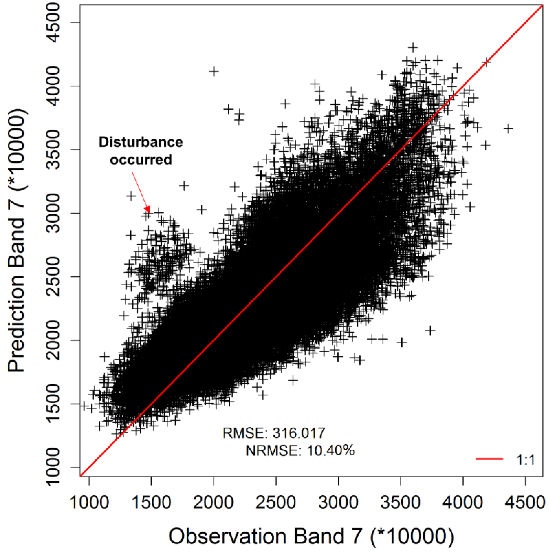
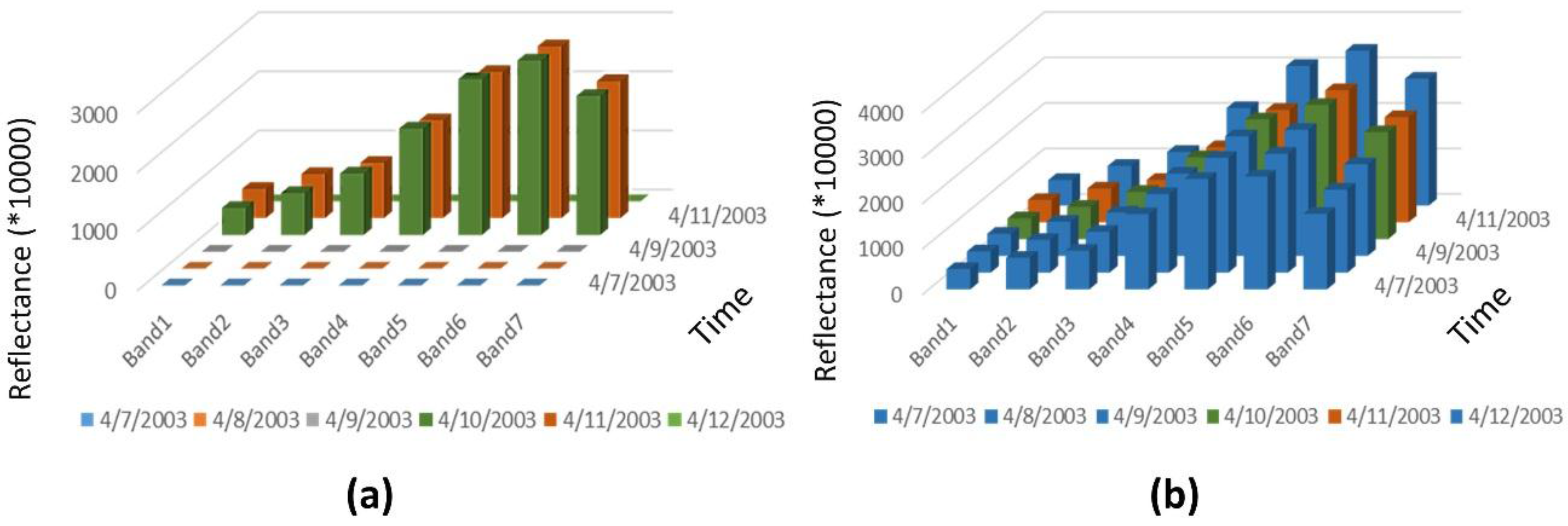
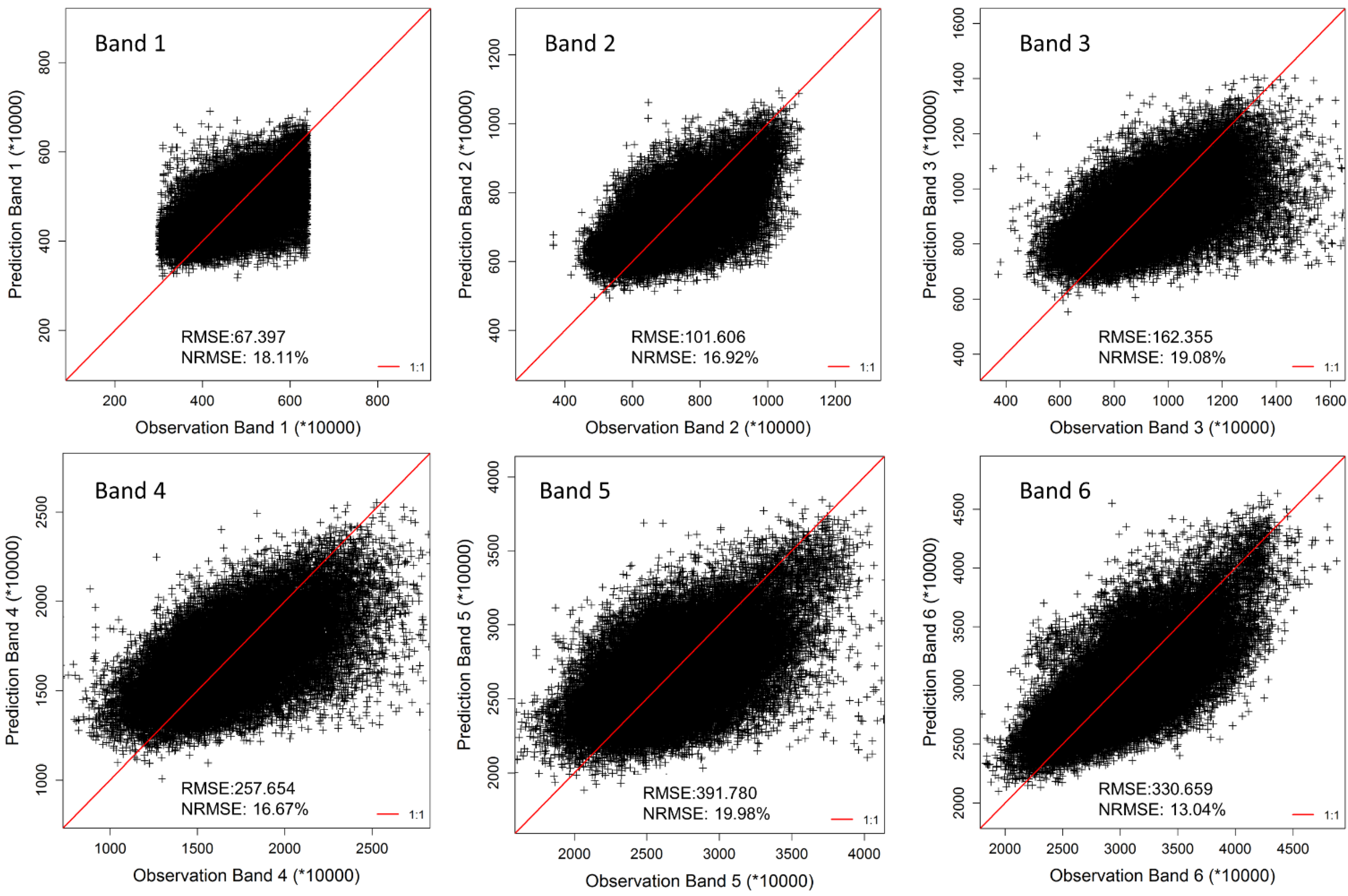
5.3. Feedback Pattern Gap Filling
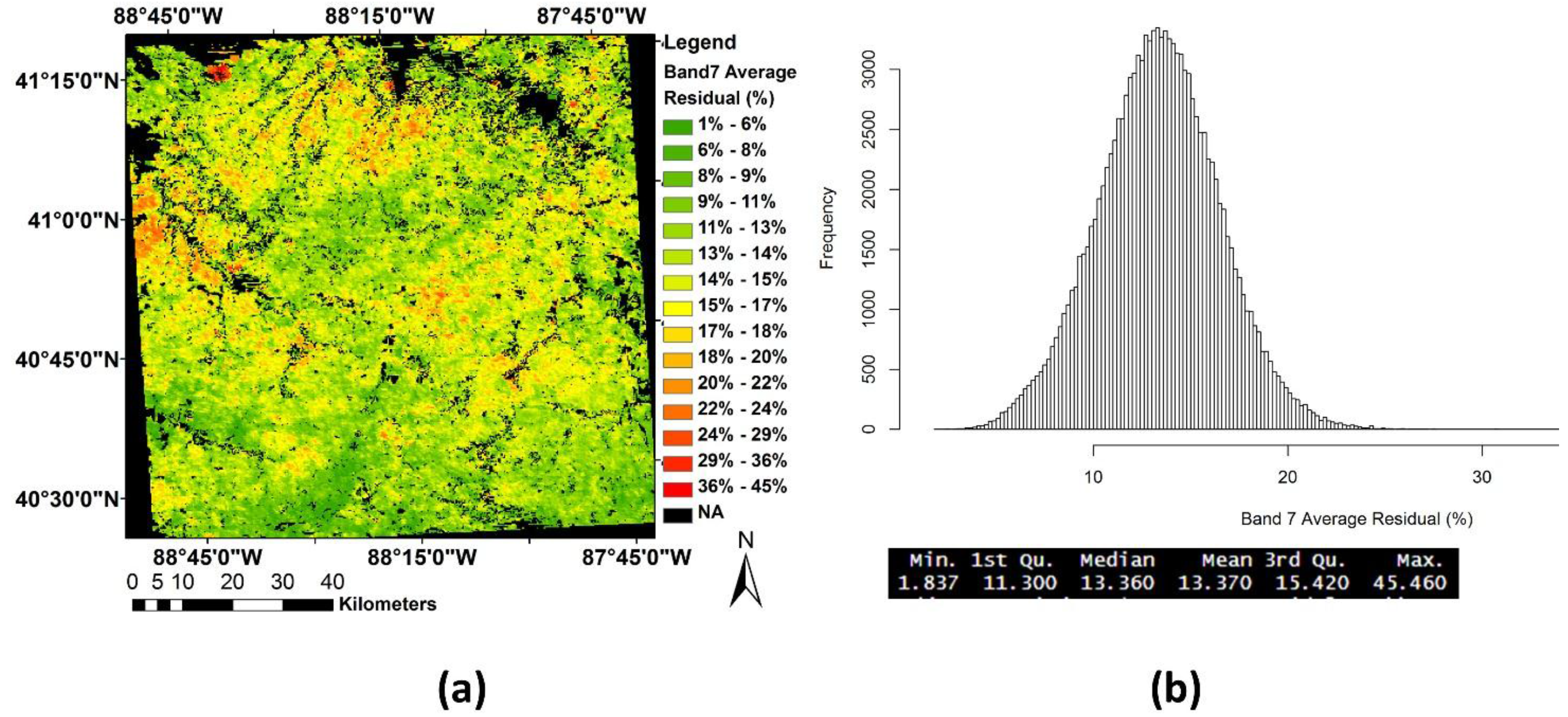
| Band 1 | Band 2 | Band 3 | Band 4 | Band 5 | Band 6 | Band 7 | |
|---|---|---|---|---|---|---|---|
| RMSE | 67.397 | 101.606 | 162.355 | 257.654 | 391.780 | 330.659 | 316.017 |
| NRMSE(%) | 18.11% | 16.92% | 19.08% | 16.67% | 19.98% | 13.04% | 10.40% |

6. Conclusions
Acknowledgments
Author Contributions
Conflicts of Interest
References
- Moran, M.S.; Inoue, Y.; Barnes, E.M. Opportunities and limitations for image-based remote sensing in precision crop management. Remote Sens. Environ. 1997, 61, 319–346. [Google Scholar] [CrossRef]
- McBratney, A.B.; Mendonça Santos, M.L.; Minasny, B. On digital soil mapping. Geoderma 2003, 117, 3–52. [Google Scholar] [CrossRef]
- Croft, H.; Anderson, K.; Kuhn, N.J. Characterizing soil surface roughness using a combined structural and spectral approach. Eur. J. Soil Sci. 2009, 60, 431–442. [Google Scholar] [CrossRef]
- Santanello, J.A.; Peters-Lidard, C.D.; Garcia, M.E.; Mocko, D.M.; Tischler, M.A.; Moran, M.S.; Thoma, D.P. Using remotely-sensed estimates of soil moisture to infer soil texture and hydraulic properties across a semi-arid watershed. Remote Sens. Environ. 2007, 110, 79–97. [Google Scholar] [CrossRef]
- Viscarra Rossel, R.A.; Walvoort, D.J.J.; McBratney, A.B.; Janik, L.J.; Skjemstad, J.O. Visible, near infrared, mid infrared or combined diffuse reflectance spectroscopy for simultaneous assessment of various soil properties. Geoderma 2006, 131, 59–75. [Google Scholar] [CrossRef]
- Anderson, K.; Croft, H. Remote sensing of soil surface properties. Prog. Phys. Geogr. 2009, 33, 457–473. [Google Scholar] [CrossRef]
- Mulder, V.L.; de Bruin, S.; Schaepman, M.E.; Mayr, T.R. The use of remote sensing in soil and terrain mapping—A review. Geoderma 2011, 162, 1–19. [Google Scholar] [CrossRef]
- Lobell, D.B.; Asner, G.P. Moisture effects on soil reflectance. Soil Sci. Soc. Am. J. 2002, 66, 722–727. [Google Scholar] [CrossRef]
- Zhu, A.-X.; Liu, F.; Li, B.; Pei, T.; Qin, C.; Liu, G.; Wang, Y.; Chen, Y.; Ma, X.; Qi, F.; et al. Differentiation of soil conditions over low relief areas using feedback dynamic patterns. Soil Sci. Soc. Am. J. 2010, 74, 861–869. [Google Scholar] [CrossRef]
- Liu, F.; Geng, X.; Zhu, A.-X.; Fraser, W.; Waddell, A. Soil texture mapping over low relief areas using land surface feedback dynamic patterns extracted from MODIS. Geoderma 2012, 171–172, 44–52. [Google Scholar] [CrossRef]
- Poggio, L.; Gimona, A.; Brown, I. Spatio-temporal MODIS EVI gap filling under cloud cover: An example in Scotland. ISPRS J. Photogramm. Remote Sens. 2012, 72, 56–72. [Google Scholar] [CrossRef]
- Roy, D.P.; Ju, J.; Lewis, P.; Schaaf, C.; Gao, F.; Hansen, M.; Lindquist, E. Multi-temporal MODIS-Landsat data fusion for relative radiometric normalization, gap filling, and prediction of Landsat data. Remote Sens. Environ. 2008, 112, 3112–3130. [Google Scholar] [CrossRef]
- Boloorani, A.D.; Erasmi, S.; Kappas, M. Multi-Source remotely sensed data combination: Projection transformation gap-fill procedure. Sensors 2008, 8, 4429–4440. [Google Scholar] [CrossRef]
- Zhang, C.; Li, W.; Travis, D. Gaps-fill of SLC-off Landsat ETM+ satellite image using a geostatistical approach. Int. J. Remote Sens. 2007, 28, 5103–5122. [Google Scholar] [CrossRef]
- Brooks, E.B.; Thomas, V.A.; Wynne, R.H.; Coulston, J.W. Fitting the multitemporal curve: A fourier series approach to the missing data problem in remote sensing analysis. IEEE Trans. Geosci. Remote Sens. 2012, 50, 3340–3353. [Google Scholar] [CrossRef]
- Pringle, M.J. Robust prediction of time-integrated NDVI. Int. J. Remote Sens. 2013, 34, 4791–4811. [Google Scholar] [CrossRef]
- NOAA National Climatic Data Center Weather Data (1981–2010). Available online: http://www.ncdc.noaa.gov/cdo-web/datatools/normals (accessed on 16 May 2014).
- Ventura, F.; Snyder, R.L.; Bali, K.M. Estimating evaporation from bare soil using soil moisture data. J. Irrig. Drain. Eng. 2006, 132, 153–158. [Google Scholar] [CrossRef]
- Muller, E.; Decamps, H. Modeling soil moisture—Reflectance. Remote Sens. Environ. 2001, 76, 173–180. [Google Scholar] [CrossRef]
- Liu, W.; Baret, F.; Gu, X.; Tong, Q.; Zheng, L.; Zhang, B. Relating soil surface moisture to reflectance. Remote Sens. Environ. 2002, 81, 238–246. [Google Scholar]
- Somers, B.; Gysels, V.; Verstraeten, W.W.; Delalieux, S.; Coppin, P. Modelling moisture-induced soil reflectance changes in cultivated sandy soils: A case study in citrus orchards. Eur. J. Soil Sci. 2010, 61, 1091–1105. [Google Scholar] [CrossRef]
- Fabre, S.; Briottet, X.; Lesaignoux, A. Estimation of soil moisture content from the spectral reflectance of bare soils in the 0.4–2.5 µm domain. Sensors 2015, 15, 3262–3281. [Google Scholar] [CrossRef] [PubMed]
- Gladkova, I.; Grossberg, M. Quantitative restoration for MODIS band 6 on Aqua. IEEE Trans. Geosci. Remote Sens. 2012, 50, 1–8. [Google Scholar] [CrossRef]
- Gallardo, M.; Snyder, R.; Schulbach, K.; Jackson, L. Crop growth and water use model for lettuce. J. Irrig. Drain. Eng. 1996, 122, 354–359. [Google Scholar] [CrossRef]
- Wythers, K.R.; Lautnroth, W.K.; Paruelo, J.M. Bare-soil evaporation under semiarid field conditions. Soil Sci. Soc. Am. J. 1999, 63, 1341–1349. [Google Scholar] [CrossRef]
- Mellouli, H.; van Wesemael, B.; Poesen, J.; Hartmann, R. Evaporation losses from bare soils as influenced by cultivation techniques in semi-arid regions. Agric. Water Manag. 2000, 42, 355–369. [Google Scholar] [CrossRef]
- Ritchie, J. Model for predicting evaporation from a row crop with incomplete cover. Water Resour. Res. 1972, 8, 1204–1213. [Google Scholar] [CrossRef]
- Suleiman, A.A.; Ritchie, J.T. Modeling soil water redistribution during second-stage evaporation. Soil Sci. Soc. Am. J. 2003, 67, 377–386. [Google Scholar] [CrossRef]
- Lal, R.; Shukla, M.K. Principles of Soil Physics; Marcel Dekker: New York, NY, USA, 2004. [Google Scholar]
- Stroosnijder, L. Soil evaporation: Test of a practical approach under semi-arid conditions. Netherlands J. Agric. Sci. 1987, 35, 417–426. [Google Scholar]
- Hargreaves, G.H.; Samami, Z.A. Reference crop evapotranspiration from temperature. Appl. Eng. Agric. 1985, 1, 96–99. [Google Scholar] [CrossRef]
- Martínez-Cob, A.; Tejero-Juste, M. A wind-based qualitative calibration of the Hargreaves ET0 estimation equation in semiarid regions. Agric. Water Manag. 2004, 64, 251–264. [Google Scholar] [CrossRef]
- Allen, R.G. FAO Irrigation and drainage paper. Irrig. Drain. 1998, 300, 64–65. [Google Scholar]
- Platnick, S.; King, M.D.; Ackerman, S.A.; Menzel, W.P.; Baum, B.A.; Riédi, J.C.; Frey, R.A. The MODIS cloud products: Algorithms and examples from terra. IEEE Trans. Geosci. Remote Sens. 2003, 41, 459–472. [Google Scholar] [CrossRef]
- Thornton, P.E.; Running, S.W.; White, M.A. Generating surfaces of daily meteorological variables over large regions of complex terrain. J. Hydrol. 1997, 190, 214–251. [Google Scholar] [CrossRef]
- William A, J. Soil Physics, 6th ed.; John Wiley: New York, NY, USA, 2004. [Google Scholar]
- Yang, W.; Wang, M.; Shi, P. Using MODIS NDVI time series to identify geographic patterns of landslides in vegetated regions. IEEE Geosci. Remote Sens. Lett. 2013, 10, 707–710. [Google Scholar] [CrossRef]
© 2015 by the authors; licensee MDPI, Basel, Switzerland. This article is an open access article distributed under the terms and conditions of the Creative Commons Attribution license (http://creativecommons.org/licenses/by/4.0/).
Share and Cite
Guo, S.; Meng, L.; Zhu, A.-X.; Burt, J.E.; Du, F.; Liu, J.; Zhang, G. Data-Gap Filling to Understand the Dynamic Feedback Pattern of Soil. Remote Sens. 2015, 7, 11801-11820. https://doi.org/10.3390/rs70911801
Guo S, Meng L, Zhu A-X, Burt JE, Du F, Liu J, Zhang G. Data-Gap Filling to Understand the Dynamic Feedback Pattern of Soil. Remote Sensing. 2015; 7(9):11801-11820. https://doi.org/10.3390/rs70911801
Chicago/Turabian StyleGuo, Shanxin, Lingkui Meng, A-Xing Zhu, James E. Burt, Fei Du, Jing Liu, and Guiming Zhang. 2015. "Data-Gap Filling to Understand the Dynamic Feedback Pattern of Soil" Remote Sensing 7, no. 9: 11801-11820. https://doi.org/10.3390/rs70911801