
Capability of Spaceborne Hyperspectral EnMAP Mission for Mapping Fractional Cover for Soil Erosion Modeling


 ,
,
Abstract
:
1. Introduction
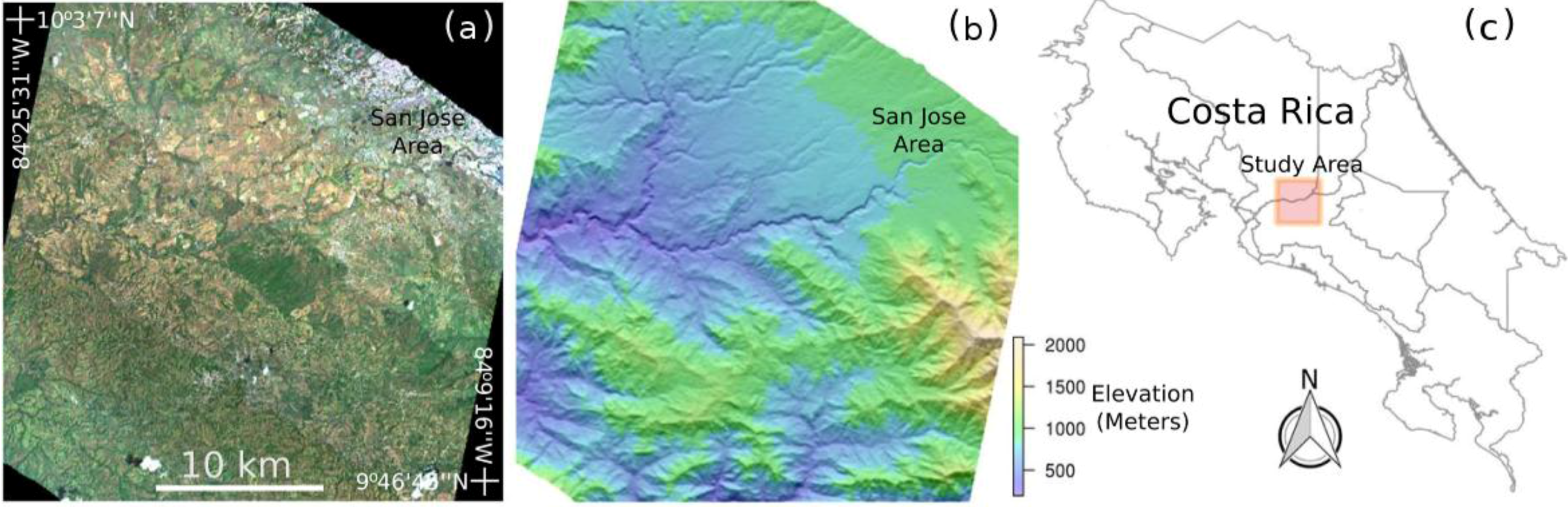
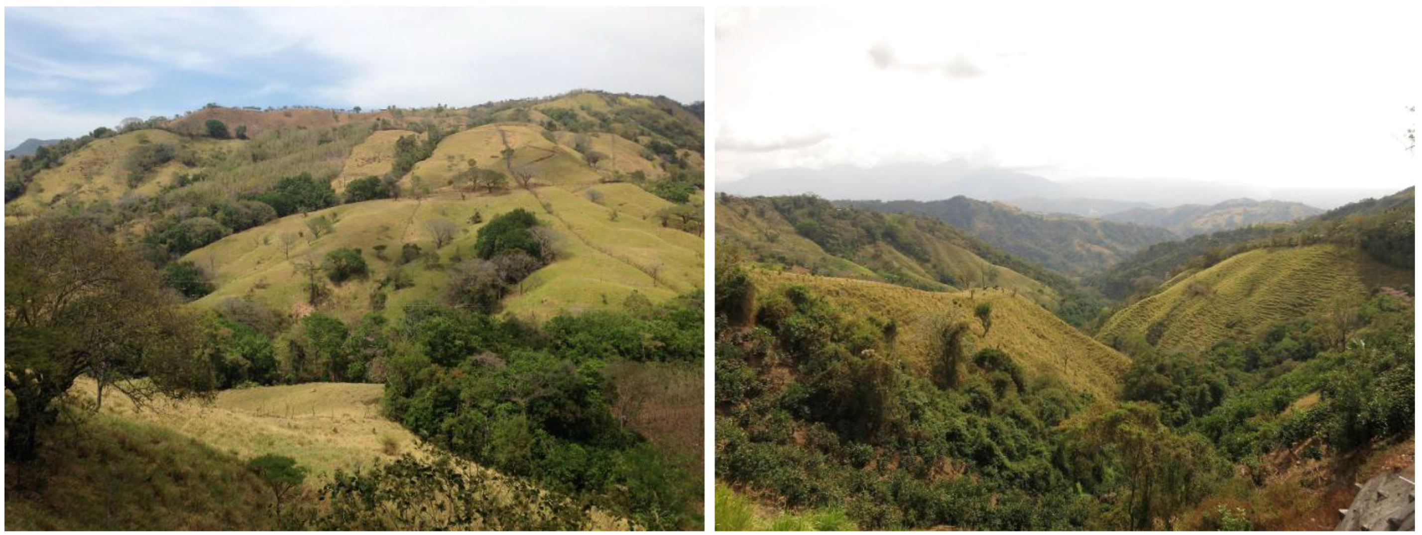
2. Study Area
3. Data
3.1. HyMap
3.2. EnMAP
4. Methodology
4.1. Fractional Cover Estimation
4.2. C-Factor Analysis
4.3. Plausibility Check Approach
5. Results
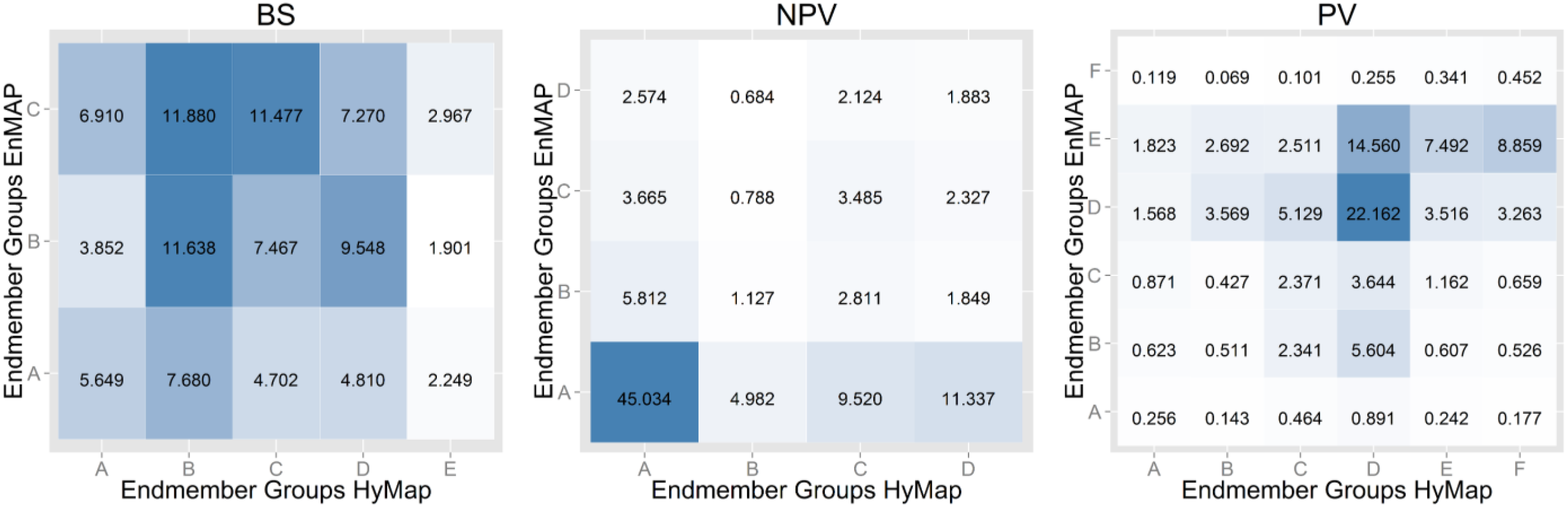
5.1. Endmember Extraction

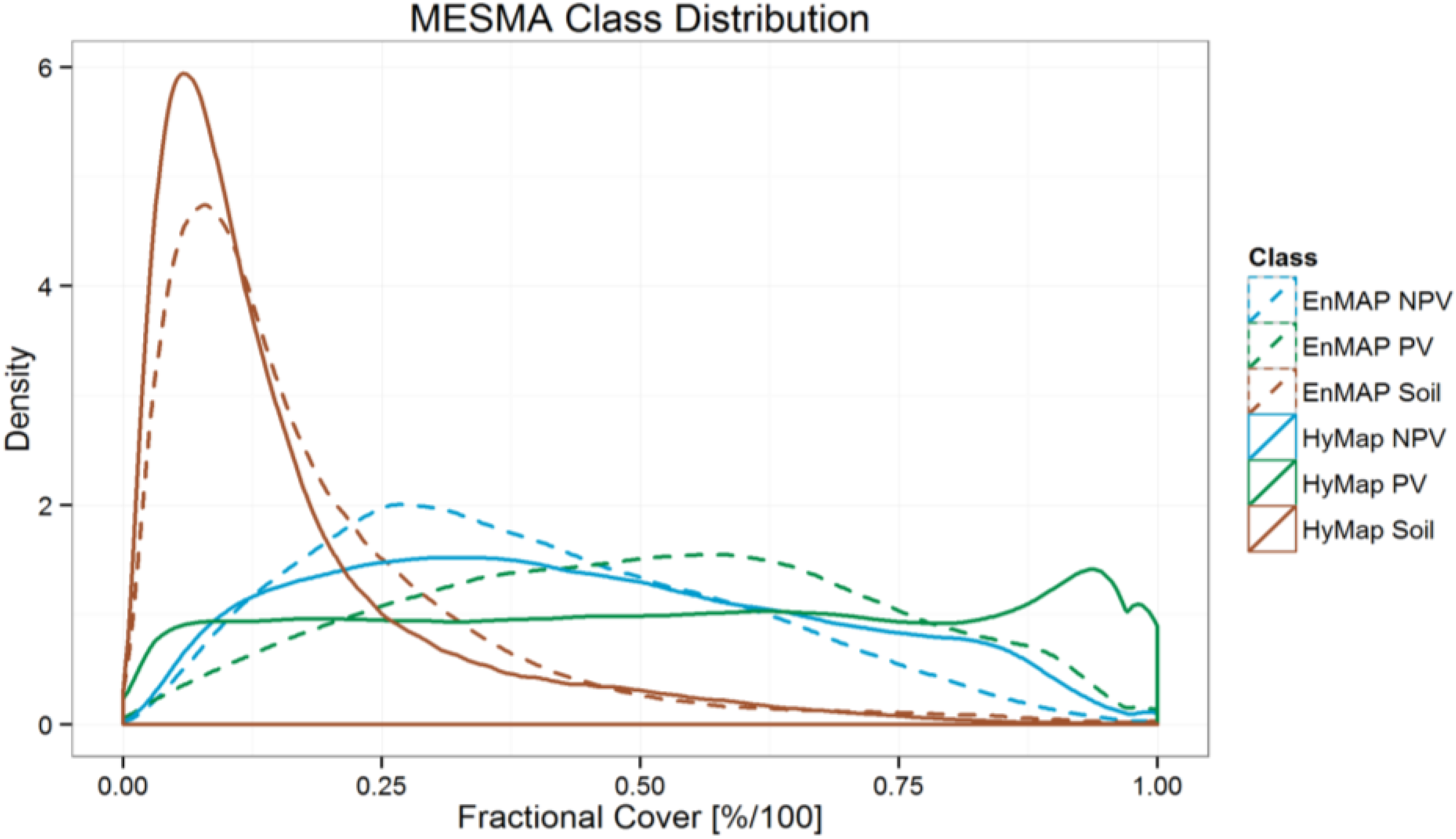
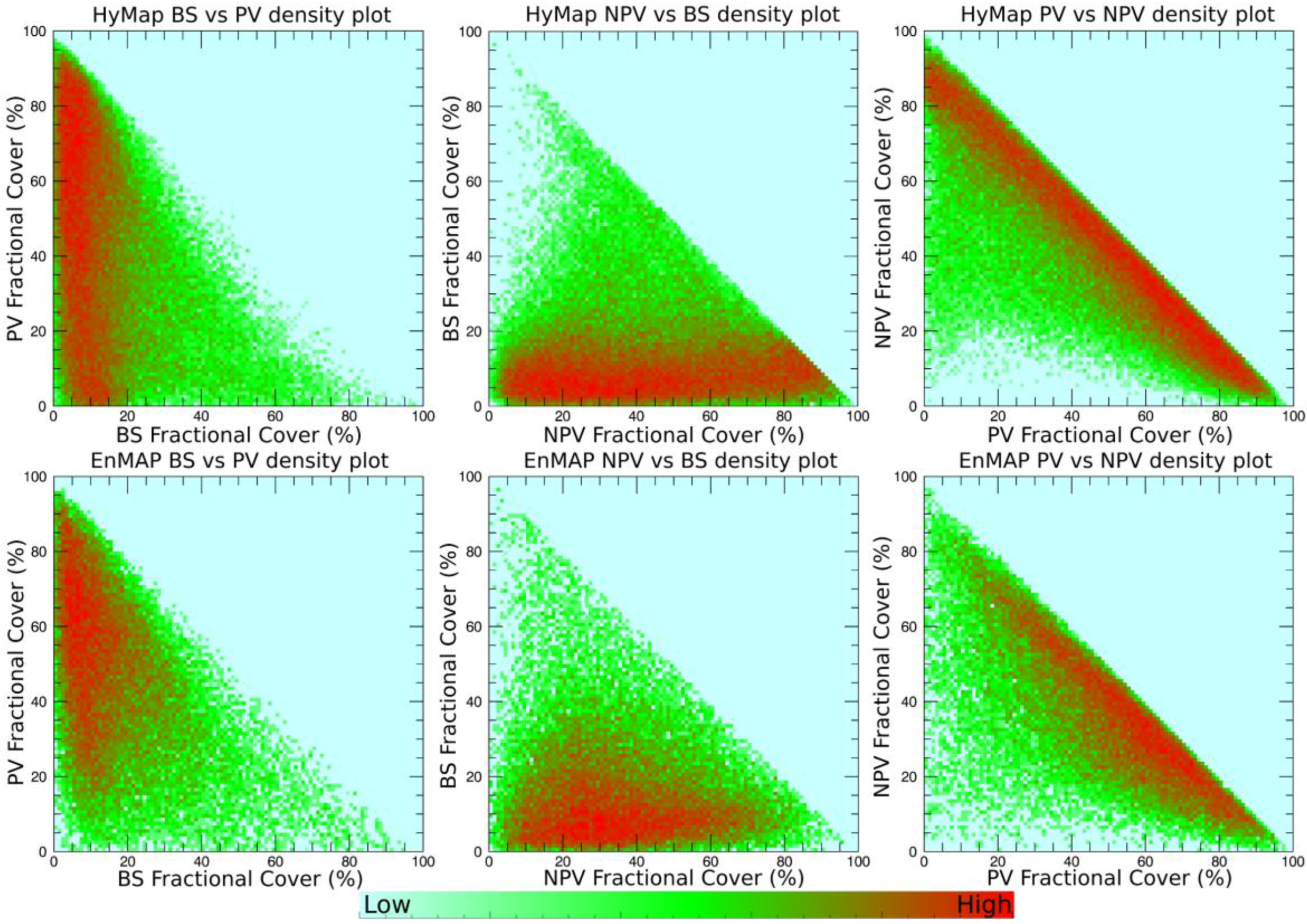
5.2. MESMA


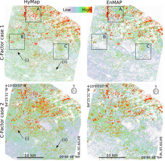
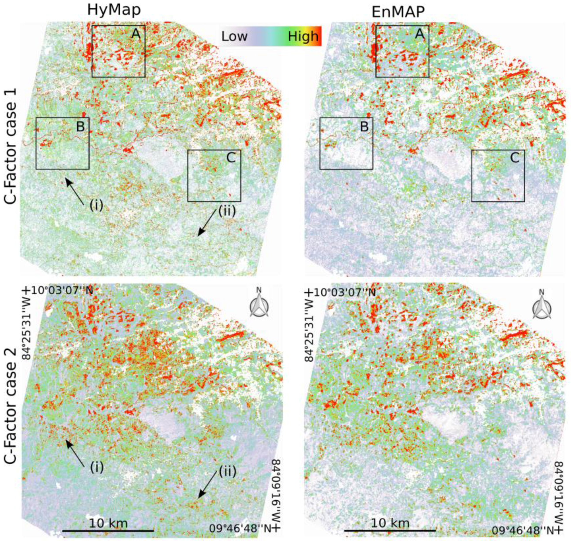
5.3. C-Factor Analysis
6. Discussion
6.1. EnMAP Simulation Quality
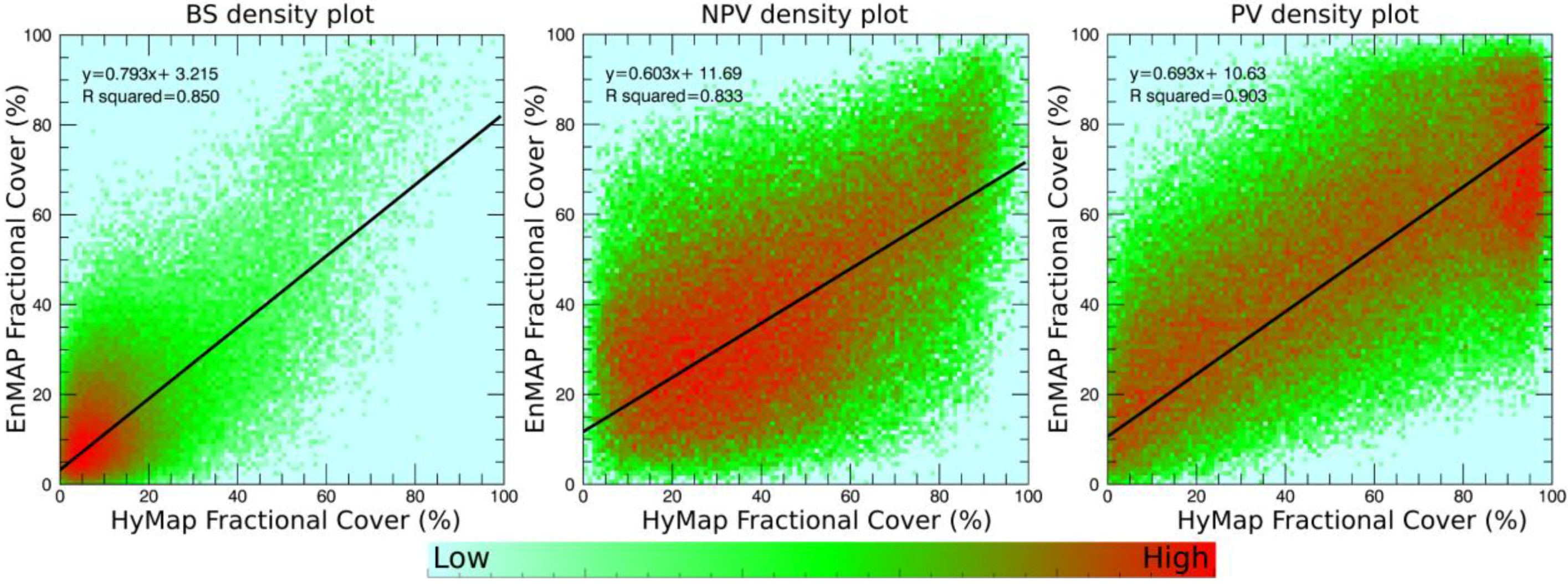
6.2. Fractional Cover Estimates
6.3. C-Factor Analysis
7. Conclusions and Outlook
Acknowledgments
Author Contributions
Conflicts of Interest
References
- Kaufmann, H.; Segl, K.; Chabrillat, S.; Hofer, S.; Stuffler, T.; Müller, A.; Richter, R.; Schreier, G; Haydn, R; Bach, H. EnMaP a hyperspectral sensor for environmental mapping and analysis (invited paper). In Proceedings of the IEEE International Geoscience and Remote Sensing Symposium, Denver, CO, USA, 31 July–4 August 2006.
- Eswaran, H.; Lal, R.; Reich, P.F. Land degradation: An overview. In Responses to Land Degradation, Proceedings of the International Conference on Land Degradation and Desertification, New Dehli, India, 2001; Hannam, I.D., Oldeman, L.R., Pening de Vries, F.W.T., Scherr, S.J., Sompatpanit, S., Eds.; Oxford Press: Oxford, UK, 2001. [Google Scholar]
- Lal, R. Soil erosion and the global carbon budget. Environ. Int. 2003, 29, 437–450. [Google Scholar] [CrossRef]
- Lee, S. Soil erosion assessment and its verification using the universal soil loss equation and geographic information system: A case study at Boun, Korea. Environ. Geol. 2004, 45, 457–465. [Google Scholar] [CrossRef]
- Vrieling, A. Satellite remote sensing for water erosion assessment. Catena 2006, 65, 2–18. [Google Scholar] [CrossRef]
- Ferreira, V.; Panagopoulos, T. Seasonality of soil erosion under Mediterranean conditions at the Alqueva dam watershed. Environ. Manag. 2014, 54, 67–83. [Google Scholar] [CrossRef] [PubMed]
- Labrière, N.; Locatelli, B.; Laumonier, Y.; Freycon, V.; Bernoux, M. Soil erosion in the humid tropics: A systematic quantitative review. Agric. Ecosyst. Environ. 2015, 203, 127–139. [Google Scholar] [CrossRef] [Green Version]
- Wischmeier, W.H.; Smith, D.D. A universal soil-loss equation to guide conservation farm planning. Trans. Int. Congr. Soil Sci. 1968, 1, 418–425. [Google Scholar]
- Morgan, R.P.C.; Quinton, J.N.; Smith, R.E.; Govers, G.; Poesen, W.A.; Auerswald, K.; Chisci, G.; Torri, D.; Styczen, M.E. The European Soil Erosion Model (EUROSEM): A dynamic approach for predicting sediment transport from fields and small catchments. Earth Surf. Process. Landf. 1998, 23, 527–544. [Google Scholar] [CrossRef]
- Gyssels, G.; Poesen, J.; Bochet, E.; Li, Y. Impact of plant root characteristics on resistance of soil to erosion by water: A review. Prog. Phys. Geogr. 2005, 29, 189–217. [Google Scholar] [CrossRef]
- De Asis, A.M.; Omasa, K. Estimation of vegetation parameter for modeling soil erosion using spectral mixture analysis of Landsat ETM data. ISPRS J. Photogramm. Remote Sens. 2007, 62, 309–324. [Google Scholar] [CrossRef]
- Gray, D.H.; Sotir, R.B. Biotechnical and Soil Bioengineering Slope Stabilization: A Practical Guide for Erosion Control; John Wiley and Sons: New York, NY, USA, 1996. [Google Scholar]
- Renard, K.G.; Yoder, D.C.; Lightle, D.T.; Dabney, S.M. Universal Soil Loss Equation and Revised Universal Soil Loss Equation, 1st ed.; Blackwell Publishing Ltd.: Oxford, UK, 2011. [Google Scholar]
- Mirsal, I.A. Soil Pollution: Origin, Monitoring and Remediation; Springer: Berlin, Heidelberg, Germany, 2008. [Google Scholar]
- Shoshanya, M.; Goldshlegerb, N.; Chudnovskyc, A. Monitoring of agricultural soil degradation by remote-sensing methods: A review. Int. J. Remote Sens. 2013, 37, 6152–6181. [Google Scholar] [CrossRef]
- Veihe, A.; Rey, J.; Quinton, J.N.; Strauss, P.; Sancho, F.M.; Somarriba, M. Modelling of event-based soil erosion in Costa Rica, Nicaragua and Mexico: Evaluation of the Eurosem model. Catena 2001, 44, 187–203. [Google Scholar] [CrossRef]
- Asner, G.P.; Knapp, D.E.; Cooper, A.N.; Bustamante, M.M.C.; Olander, L.P. Ecosystem structure throughout the brazilian amazon from landsat observations and automated spectral unmixing. Earth Interact. 2005, 9, 1–31. [Google Scholar] [CrossRef]
- Guerschman, J.P.; Scarth, P.F.; McVicar, T.R.; Renzullo, L.J.; Malthus, T.J.; Stewart, J.B.; Rickards, J.E.; Trevithick, R. Assessing the effects of site heterogeneity and soil properties when unmixing photosynthetic vegetation, non-photosynthetic vegetation and BS fractions from Landsat and MODIS data. Remote Sens. Environ. 2015, 161, 12–26. [Google Scholar] [CrossRef]
- Okin, G.S.; Clarke, K.D.; Lewis, M.M. Comparison of methods for estimation of absolute vegetation and soil fractional cover using MODIS normalized BRDF-adjusted reflectance. Remote Sens. Environ. 2013, 130, 266–270. [Google Scholar] [CrossRef]
- Okin, G.S. Relative spectral mixture analysis—A multitemporal index of total vegetation cover. Remote Sens. Environ. 2007, 106, 467–479. [Google Scholar] [CrossRef]
- Asner, G.P.; Heidebrecht, K.B. Spectral unmixing of vegetation, soil and dry carbon in arid regions: Comparing multi-spectral and hyperspectral observations. Int. J. Remote Sens. 2002, 23, 400–410. [Google Scholar] [CrossRef]
- Asner, G.P.; Lobell, D.B. A biogeophysical approach for automated SWIR unmixing of soils and vegetation. Remote Sens. Environ. 2000, 74, 99–112. [Google Scholar] [CrossRef]
- Elvidge, C.D. Visible and near infrared reflectance characteristics of dry plant materials. Int. J. Remote Sens. 1990, 11, 1775–1795. [Google Scholar] [CrossRef]
- Ustin, S.L.; Roberts, D.A.; Gamon, J.A.; Asner, G.P.; Green, R.O. Using imaging spectroscopy to study ecosystem processes and properties. Bio. Sci. 2004, 54, 523–534. [Google Scholar] [CrossRef]
- Ben-Dor, E.; Chabrillat, S.; Dematte, J.A.M.; Taylor, G.R.; Hill, J.; Whiting, M.L.; Sommer, S. Using imaging spectroscopy for soil properties. Remote Sens. Environ. 2009, 113, S38–S55. [Google Scholar] [CrossRef]
- Nocita, M.; Stevens, A.; van Wesemael, B.; Aitkenhead, M.; Bachmann, M.; Barthes, B.; Ben-Dor, E.; Brown, D.J.; Clairotte, M.; Csorba, A.; et al. Spectroscopy: An alternative to wet chemistry for soil monitoring. Adv. Agron. 2015, 132, 1–21. [Google Scholar]
- Daughtry, C.S.T.; Doraiswamy, P.C.; Hunt, E.R., Jr.; Stern, A.J.; McMurtrey, J.E., III; Prueger, J.H. Remote sensing of crop residue cover and soil tillage intensity. Soil Tillage Res. 2006, 91, 101–108. [Google Scholar] [CrossRef]
- Delegido, J.; Verrelst, J.; Rivera, J.P.; Ruiz-Verdu, A.; Moreno, J. Brown and green LAI mapping through spectral indices. Int. J. Appl. Earth Obs. Geoinform. 2015, 35, 350–358. [Google Scholar] [CrossRef]
- Mulder, V.L.; de Bruin, S.; Schaepman, M.E.; Mayr, T.R. The use of remote sensing in soil and terrain mapping—A review. Geoderma 2011, 162, 1–19. [Google Scholar] [CrossRef]
- Förster, S.; Wilczok, C.; Brosinsky, A.; Segl, K. Assessment of sediment connectivity from vegetation cover and topography using remotely sensed data in a dryland catchment in the Spanish Pyrenees. J. Soil. Sediment. 2014, 14, 1982–2000. [Google Scholar] [CrossRef]
- Bayer, A.; Bachmann, M.; Müller, A.; Kaufmann, H. A comparison of feature-based MLR and PLS regression techniques for the prediction of three soil constituents in a degraded South African ecosystem. Appl. Environ. Soil Sci. 2012, 2012, 1–20. [Google Scholar] [CrossRef]
- Okin, G.; Roberts, D.; Murray, B.; Okin, W. Practical limits on hyperspectral vegetation discrimination in arid and semiarid environments. Remote Sens. Environ. 2001, 77, 212–225. [Google Scholar] [CrossRef]
- Bannari, A.; Staenz, K.; Champagne, C.; Khurshid, K.S. Spatial variability mapping of crop residue using Hyperion (EO-1) hyperspectral data. Remote Sens. 2015, 7, 8107–8127. [Google Scholar] [CrossRef]
- Ghosh, G.; Kumar, S.; Saha, S.K. Hyperspectral satellite data in mapping salt-affected soils using linear spectral unmixing analysis. J. Indian Soc. Remote Sens. 2012, 40, 129–136. [Google Scholar] [CrossRef]
- Wu, J.; Liu, Y.; Wang, J.; He, T. Application of Hyperion data to land degradation mapping in the Hengshan region of China. Int. J. Remote Sens. 2010, 31, 5145–5161. [Google Scholar] [CrossRef]
- Kruse, F.A.; Boarsmann, J.W.; Huntingtin, J.F. Comparison of airborne hyperspectral data and EO-1 Hyperion for mineral mapping. IEEE Trans. Geosci. Remote Sens. 2003, 41, 1388–1400. [Google Scholar] [CrossRef]
- Roberts, D.A.; Dennison, P.E.; Gardner, M.E.; Hetzel, Y.; Ustin, S.L.; Lee, C.T. Evaluation of the potential of Hyperion for fire danger assessment by comparison to the airborne visible/infrared imaging spectrometer. IEEE Trans. Geosci. Remote Sens. 2003, 41, 1297–1320. [Google Scholar] [CrossRef]
- Middleton, E.M.; Ungar, S.G.; Mandl, D.J.; Ong, L.; Frye, S.W.; Campbell, P.E.; Landis, D.R.; Young, J.P.; Pollack, N.H. The earth observing one (EO-1) satellite mission: Over a decade in space. IEEE J. Sel. Top. Appl. Earth Obs. Remote Sens. 2013, 6, 243–256. [Google Scholar] [CrossRef]
- Guanter, L.; Kaufmann, H.; Segl, K.; Foerster, S.; Rogass, C.; Chabrillat, S.; Kuester, T.; Hollstein, A.; Rossner, G.; Chlebek, C.; et al. The Environmental Mapping and Analysis Program (EnMAP) spaceborne imaging spectroscopy mission for Earth observation. Remote Sens. 2015, 7, 8830–8857. [Google Scholar] [CrossRef]
- Roberts, D.A.; Quattrochi, D.A.; Hulley, G.C.; Hook, S.J.; Green, R.O. Synergies between VSWIR and TIR data for the urban environment: An evaluation of the potential for the hyperspectral infrared imager (HyspIRI) decadal survey mission. Remote Sens. Environ. 2012, 117, 83–101. [Google Scholar] [CrossRef]
- Matsunaga, T.; Iwasaki, A.; Tsuchida, S.; Tanii, J.; Kashimura, O.; Nakamura, R.; Yamamoto, H.; Tachikawa, T.; Rokugawa, S. Current status of Hyperspectral Imager Suite (HISUI). In Peoceedings of the IEEE Geoscience and Remote Sensing Symposium, Melbourne, Australia, 21–26 July 2013; pp. 3510–3513.
- Segl, K.; Guanter, L.; Rogaß, C.; Küster, T.; Roessner, S.; Kaufmann, H.; Sang, B.; Mogulsky, V.; Hofer, S. Eetes- the EnMAP end-to-end simulation tool. IEEE Trans. Geosci. Remote Sens. 2012, 5, 522–530. [Google Scholar] [CrossRef]
- Rogge, D.; Rivard, B.; Segl, K.; Grant, B.; Feng, J. Mapping of NiCu–PGE ore hosting ultramafic rocks using airborne and simulated EnMAP hyperspectral imagery, Nunavik, QC, Canada. Remote Sens. Environ. 2014, 152, 302–317. [Google Scholar] [CrossRef]
- Soil Conservation Service. In Soil Taxonomy: A Basic System of Soil Classification for Making and Interpreting Soil Surveys, 2nd ed.; U.S. Department of Agriculture Handbook 436; Natural Resources Conservation Service: Washington, DC, USA, 10 August 1999.
- Bachmann, M.; Habermeyer, M.; Holzwarth, S.; Richter, R.; Müller, A. Including quality measures in an automated processing chain for airborne hyperspectral data. In Proceedings of the 5th EARSel Workshop on Imaging Spectroscopy, Bruges, Belgium, 23–25 April 2007.
- Richter, R.; Schlapfer, D. Atmospheric/Topographical Correction for Airborne Imagery: ATCOR-4 User Guide; DLR IB: Wessling, Germany, 2010. [Google Scholar]
- Müller, R.; Lehner, M.; Müller, R.; Reinartz, P.; Schroeder, M.; Vollmer, B. A program for direct georeferencing of airborne and spaceborne line scanner images. In Proceedings of the International Archives of Photogrammetry Remote Sensing and Spatial Information Sciences, Denver, CO, USA, 10–15 November 2002; pp. 148–153.
- Schläpfer, D.; Richter, R.; Feingersh, T. Operational BRDF effects correction for wide-field-of-view optical scanners (BREFCOR). IEEE Trans. Geosci. Remote Sens. 2015, 53, 1855–1864. [Google Scholar] [CrossRef]
- Guanter, L.; Segl, K.; Kaufmann, H. Simulation of the optical remote-sensing scenes with application to the EnMAP hyperspectral mission. IEEE Trans. Geosci. Remote Sens. 2009, 47, 2340–2351. [Google Scholar] [CrossRef]
- Segl, K.; Guanter, L.; Kaufmann, H.; Schubert, J.; Kaiser, S.; Sang, B.; Hofer, S. Simulation of spatial sensor characteristics in the context of the EnMAP hyper-spectral mission. IEEE Trans. Geosci. Remote Sens. 2010, 48, 3046–3054. [Google Scholar] [CrossRef]
- Esch, T.; Marconcini, M.; Felbier, A.; Roth, A.; Heldens, W.; Huber, M; Schwinger, M.; Taubenböck, H.; Müller, A.; Dech, S. Urban footprint processor—Fully automated processing chain generating settlement masks from global data of the TanDEM-X mission. IEEE Geosci. Remote Sens. Lett. 2013, 10, 1617–1621. [Google Scholar] [CrossRef]
- Adams, J.B.; Smith, M.O.; Gillespie, A.R. Imaging spectroscopy: Interpretation based on spectral mixture analysis. In Remote Geochemical Analysis: Elemental and Mineralogical Composition; Pieters, C.M., Englert, P.A., Eds.; Cambridge University Press: Cambridge, UK, 1993; pp. 145–166. [Google Scholar]
- Rogge, D.; Bachmann, M.; Rivard, B.; Feng, J. Spatial sub-sampling using local endmembers for adapting OSP and SSEE for large-scale hyperspectral surveys. IEEE J. Sel. Topics Appl. Earth Obs. Remote Sens. 2012, 5, 183–195. [Google Scholar] [CrossRef]
- Price, J.C. How unique are spectral signatures? Remote Sens. Environ. 1994, 49, 181–186. [Google Scholar] [CrossRef]
- Roberts, D.; Gardner, M.; Church, R.; Ustin, S.; Scheer, G.; Green, R. Mapping chaparral in the Santa Monica Mountains using multiple endmember spectral mixture models. Remote Sens. Environ. 1998, 65, 267–279. [Google Scholar] [CrossRef]
- Bachmann, M. Automated Estimation of Ground Cover Fractions Using MESMA Unmixing. Ph.D. Thesis, University of Wuerzburg, Wuerzburg, Germany, December 2007. [Google Scholar]
- Bachmann, M.; Müller, A.; Dech, S. Increasing and evaluating the reliability of multiple endmember spectral mixture analysis (MESMA). In Proceedings of the 6th EARSeL-SIG-IS, Tel Aviv, Israel, 16–19 March 2009.
- Zabcic, N.; Rivard, B.; Ong, C.; Müller, A. Using airborne hyperspectral data to characterize the surface pH and mineralogy of pyrite mine tailings. Int. J. Appl. Earth Obs. Geoinform. 2014, 32, 152–162. [Google Scholar] [CrossRef]
- Mitra, B.; Scotta, H.D.; Dixon, J.C.; McKimmey, J.M. Applications of fuzzy logic to the prediction of soil erosion in a large watershed. Geoderma 1998, 86, 183–209. [Google Scholar] [CrossRef]
- Bakimchandra, O. Integrated Fuzzy-GIS Approach for Assessing Regional Soil Erosion Risks. Ph.D. Thesis, University of Stuttgart, Stuttgart, Germany, August 2011. [Google Scholar]
- Wischmeier, W.H.; Smith, D.D. Predicting Rainfall Erosion Losses—A Guide to Conservation Planning; Agriculture Handbook No. 537; U.S. Department of Agriculture: Washington, DC, USA, December 1978. [Google Scholar]
- Thorp, K.R.; French, A.N.; Rango, A. Effect of image spatial and spectral characteristics on mapping semi-arid rangeland vegetation using multiple endmember spectral mixture analysis (MESMA). Remote Sens. Environ. 2013, 132, 120–130. [Google Scholar] [CrossRef]
- Okujeni, A.; van der Linden, S.; Hostert, P. Extending the vegetation-impervious-soil model using simulated EnMAP data and machine learning. Remote Sens. Environ. 2015, 158, 69–80. [Google Scholar] [CrossRef]
© 2015 by the authors; licensee MDPI, Basel, Switzerland. This article is an open access article distributed under the terms and conditions of the Creative Commons Attribution license (http://creativecommons.org/licenses/by/4.0/).
Share and Cite
Malec, S.; Rogge, D.; Heiden, U.; Sanchez-Azofeifa, A.; Bachmann, M.; Wegmann, M. Capability of Spaceborne Hyperspectral EnMAP Mission for Mapping Fractional Cover for Soil Erosion Modeling. Remote Sens. 2015, 7, 11776-11800. https://doi.org/10.3390/rs70911776
Malec S, Rogge D, Heiden U, Sanchez-Azofeifa A, Bachmann M, Wegmann M. Capability of Spaceborne Hyperspectral EnMAP Mission for Mapping Fractional Cover for Soil Erosion Modeling. Remote Sensing. 2015; 7(9):11776-11800. https://doi.org/10.3390/rs70911776
Chicago/Turabian StyleMalec, Sarah, Derek Rogge, Uta Heiden, Arturo Sanchez-Azofeifa, Martin Bachmann, and Martin Wegmann. 2015. "Capability of Spaceborne Hyperspectral EnMAP Mission for Mapping Fractional Cover for Soil Erosion Modeling" Remote Sensing 7, no. 9: 11776-11800. https://doi.org/10.3390/rs70911776