Article

A Weighted Algorithm Based on Normalized Mutual Information for Estimating the Chlorophyll-a Concentration in Inland Waters Using Geostationary Ocean Color Imager (GOCI) Data

1
International Institute for Earth System Science, Nanjing University, Nanjing 210023, China
2
Jiangsu Provincial Key Laboratory of Geographic Information Science and Technology, Nanjing University, Nanjing 210023, China
3
Jiangsu Center for Collaborative Innovation in Geographical Information Resource Development and Application, Nanjing 210023, China
4
Institute of Space and Earth Information Science, The Chinese University of Hong Kong, Shatin, Hong Kong, China
5
Key Laboratory of Virtual Geographic Environment, Nanjing Normal University, Ministry of Education, Nanjing 210023, China
*
Author to whom correspondence should be addressed.
These authors contributed equally to this work.
Remote Sens. 2015, 7(9), 11731-11752; https://doi.org/10.3390/rs70911731
Submission received: 6 August 2015 / Revised: 30 August 2015 / Accepted: 8 September 2015 / Published: 14 September 2015
(This article belongs to the Special Issue Remote Sensing of Water Resources)

Abstract

:
Due to the spatiotemporal variations of complex optical characteristics, accurately estimating chlorophyll-a (Chl-a) concentrations in inland waters using remote sensing techniques remains challenging. In this study, a weighted algorithm was developed to estimate the Chl-a concentrations based on spectral classification and weighted matching using normalized mutual information (NMI). Based on the NMI algorithm, three water types (Class 1 to Class 3) were identified using the in situ normalized spectral reflectance data collected from Taihu Lake. Class-specific semi-analytic algorithms for the Chl-a concentrations were established based on the GOCI data. Next, weighted factors, which were used to determine the matching probabilities of different water types, were calculated between the GOCI data and each water type using the NMI algorithm. Finally, Chl-a concentrations were estimated using the weighted factors and the class-specific inversion algorithms for the GOCI data. Compared to the non-classification and hard-classification algorithms, the accuracies of the weighted algorithms were higher. The mean absolute error and root mean square error of the NMI weighted algorithm decreased to 22.63% and 9.41 mg/m3, respectively. The results also indicated that the proposed algorithm could reduce discontinuous or jumping effects associated with the hard-classification algorithm.

Graphical Abstract

1. Introduction

Lake eutrophication, which is characterized by algal blooms, has become one of the most serious environmental issues around the world [1,2]. Not only do algal blooms cause the degradation of aquatic ecosystems, but the toxins produced by the algae also threaten human and animal health [3]. As a basic indicator of phytoplankton biomass, the chlorophyll-a concentration plays a significant role in indicating the status of algal pollution and the trophic condition of a water body [4,5].
The Chl-a concentration can be estimated using remote sensing data due to its unique spectral properties [4,6]. For Case I water (i.e., open oceans), algorithms based on blue and green spectral reflectances can be used due to the relatively simple optical properties [4,7]. However, optical properties of Case II waters (i.e., turbid coastal and inland waters) are influenced by complex optical components such as phytoplankton, total suspended matter (TSM) and colored, dissolved organic matter (CDOM); thus, the blue-green algorithms may not be suitable for this type of water [8]. Due to this problem, effective semi-empirical algorithms using the near-infrared-red (NIR) and red spectral reflectances have been established to estimate Chl-a in Case II waters. In addition, commonly used algorithms, such as two-band and three-band algorithms, have been widely used for Case II waters in different regions [8,9,10,11].
Although various studies have assessed the potential of NIR-red algorithms to estimate the Chl-a concentration using satellite images in Case II waters [8,12], the results are usually obtained from the universal models that are separately established for different study regions or different seasons. However, the distribution of the relevant optical components is heterogeneous, and the optical properties of water vary due to human influence, wind speed and direction or the topography of the bed in the same body of water [4,5,13]. Therefore, it is difficult to use a single model to estimate the Chl-a concentration in optically complex water [14]. Algorithms based on universal models are defined as non-classification algorithms in this study. To address this problem, approaches based on water optical classification that were independent of time and region were developed to improve the inversion accuracy of the water quality parameters [15,16].
In recent years, hard classification, which classified the matching spectral reflectance to one specific optical type of inland waters and applied the class-specific retrieval algorithm to that type, was used to estimate certain water quality parameters (i.e., Chl-a, TSM) [4,5,17]. The main procedure usually included the in situ reflectance classification and remote-sensing reflectance matching. In the first step, a feature-based method based on the diagnosable spectral characteristics and a supervised or unsupervised method based on the optical properties and biogeochemical parameters of water are common approaches for in situ water optical classification [14,18,19]. Then, optimum estimation models were separately established for each optical type. In the next step, the remote-sensing reflectance was matched to one specific optical type based on the spectral properties of each in situ optical class or the distance functions between the remote-sensing reflectance and the optical classes identified from the in situ reflectance [4,13]. The class-specific inversion algorithm was subsequently applied for each remote-sensing reflectance. Previous studies indicated that the estimation accuracies of Chl-a or the TSM estimation could been improved based on the hard-classification approach in optically complex waters [4,15,18]. However, due to the fuzzy boundaries between the different classes, similar spectral reflectances might belong to different water types, or the spectral reflectance might not be completely consistent with the specific reflectance spectra of each type, resulting in different estimations of the Chl-a or TSM concentration [16]. The hard classification algorithm could produce discontinuous or jumping effects of the estimation results [15,16]. Although Moore applied blending algorithms to avoid discontinuities or the jumping effect in the coastal waters of a UNH lake, and Zhang showed that accuracies are improved based on a soft classification using the in situ data [15,20], further study of the classification, the weighted matching methods and the application results is still required.
In this study, normalized mutual information was proposed for the in situ reflectance classification and the satellite remote-sensing reflectance class matching. NMI is an improvement of the mutual information (MI), which is used to measure the statistical dependence of random variables to avoid certain misclassifications [21,22]. Studies have shown that NMI can be applied as a similarity measurement to classify the spectral reflectance [21,23,24]. Thus, a procedure, which is based on the NMI criterion for the in situ reflectance classification, the GOCI reflectance weighted matching and the weighted inversion algorithms were developed to estimate the Chl-a concentration in inland waters.
Therefore, in this study, a NMI weighting algorithm was proposed to estimate the Chl-a concentration based on the optical classification and weighted retrieval algorithms. The primary objectives of this study were: (1) to identify the optical water types using the criterion function NMI based on the in situ spectral reflectance; (2) to estimate the Chl-a concentration using a weighted algorithm based on weighting factors and to assess the accuracy of the proposed algorithm by comparison with the non-classification and hard classification algorithms; and (3) to demonstrate the potential of the proposed algorithm using GOCI data.

2. Materials

2.1. Study Area

Taihu Lake is the third largest freshwater lake in China with a surface area of 2338 km2 and an average depth of 1.9 m [25]. The lake (30°55′–31°33′N, 119°54′–120°36′E), which is located in the Yangtze River Delta, is an important water source for Jiangsu, Zhejiang and Shanghai Provinces [4,5]. Due to its advantageous location, the Taihu Lake Basin has been one of the most developed areas in China [26]. However, with the rapid economic development occurring in China recently, a significant amount of nutrients from industrial wastewater, domestic wastewater and chemical fertilizers are being directly transported into Taihu Lake, resulting in a water environment in the lake that is excellent for algae; the resulting spatial distribution of algae has been shown to be heterogeneous [4,27]. In recent years, algae blooms have occurred with increasing frequency and are distributed over larger areas. The lake has gradually become one of the three most eutrophic lakes in China.

2.2. In Situ Data

2.2.1. Samples Collection and Datasets Used

Field surveys were performed in October and November 2010; March, September, and December 2011; and May 2012. Surface water samples were recorded by a handheld Global Positioning System (GPS). At each sampling station, field spectra were measured and water samples were collected with Niskin sampling bottles. Then, all of the water samples were taken back to the laboratory under freezing conditions; Chl-a and TSM analyses were then conducted within one day. After deleting outliers, 30, 52, 48, 31 and 71 samples were, respectively, obtained separately for research during the months mentioned above. To establish and assess the class-specific inversion algorithm of the Chl-a concentration, all of the samples were randomly divided into two parts. One fourth of the samples were used to validate the NMI weighted algorithm, while the other 170 samples were applied to the calibration of the Chl-a NIR-red estimation models.

2.2.2. Reflectance Measurements

Measurements of the reflectance spectra (Rrs) were performed in the 350–1050 nm spectral range with a 1.5 nm spectral interval using an ASD FieldSpec spectroradiometer (Analytical Devices, Inc., Boulder, CO). Based on the method introduced in references [27,28], the instrument was positioned with restricted angles to minimize the effects of sunglint and the shading of ships. The azimuth view angle was between 90°–135°, and the zenith view angle was approximately 30°–40° [29]. After the measurement of the water radiance, the instrument was rotated upwards by 90°–120° to obtain the skylight radiance. During this measurement, the upwelling radiance from the water surface (Lsw), the standard gray reference board radiance (Lp) and the skylight radiance (Lsky) were recorded five times for each sample. Then, the remote sensing reflectances (Rrs) could be calculated as:
R r s = ρ p ( L s w r L s k y ) π L p
where ρ P is the reflectance of the standard gray reference board and r represents the reflectance of the skylight at the air/water interface, which was assumed to be 0.026 [5].

2.2.3. Laboratory Analysis

Surface water samples were collected for the measurement of the Chl-a, TSM, ISM (inorganic suspended matter), OSM (organic suspended matter) concentrations and aCDOM(λ). Chl-a was extracted from the GF/C filters with ethanol (90%) at 80°C. Its concentration was then corrected for pheophytin pigments and determined spectrophotometrically [4,30,31]. The concentrations of TSM were determined by filtering the water samples on pre-combusted Whatman GF/F filters, which were then dried at 105 °C for 4 h. The filters were then re-combusted and re-weighed to measure the ISM present. Then, the OSM was obtained based on the difference between the TSM and the OSM [4]. The aCDOM(λ) of each filtrate was measured by a spectrophotometer, and the procedure and calculation equation were detailed in [32] and [4].

2.3. Satellite Data

GOCI images obtained on 3 September 2011 were used as the data sources in this study [33]. The geostationary satellite GOCI was launched in 2010 and provides images with a resolution of 500 m. The sensor includes 8 spectral bands, which are between 400 and 900 nm (Table 1), and the revisit period is 1 hour (8:16 a.m. to 3:16 p.m.). Due to the high time resolution, GOCI data not only reduce the influence of clouds, but also provide data sources for short-term monitoring. To monitor dynamic variation of Chl-a concentration in inland waters, it is suitable to use GOCI data to study its spatial-diurnal distribution. Preliminary studies have shown significant potential for use in water quality parameters in turbid waters [8,34,35].
Table 1. Spectral bands of GOCI data.
BandCentral Wavelength (nm)Band Width (nm)SNRType
1412201000Visible
2443201090Visible
3490201170Visible
4555201070Visible
5660201010Visible
668010870Visible
774520860NIR
886540750NIR
Note: SNR indicates a signal-to-noise ratio.

3. Methods

The NMI weighted algorithm was developed to estimate the Chl-a concentration from GOCI data; Figure 1 shows the flowchart of the proposed algorithm. In the first step, the in situ Rrs were denoised and normalized before classification (Section 3.1). Next, the criterion function (NMI) was calculated between the pairwise normalized Rrs, and the 1-NMI was used as a distance function for Rrs classification (Section 3.2). Then, hierarchical clustering was applied to classify the in situ data (Class 1, Class 2, …, Class m) based on the distance function. The standard reflectance spectra of each class was calculated by the average of the spectra of Class i (i=1, 2, …, m ). After resampling the classified Rrs into the GOCI band, NIR-red models were established separately for the m types (Cchl-a,i,i=1, 2,…, m). Finally, weighting factors between the validation data and each class were calculated based on the NMI algorithm. The Chl-a concentration could be estimated by Cchl-a,i and the weighting factors of each type (Section 3.3). The accuracy of the NMI algorithm was assessed based on Section 3.4.
Figure 1. Flowchart of the estimation of Chl-a based on the NMI classification and the weighted algorithm.
Remotesensing 07 11731 g001

3.1. Pre-Treatment of Data

3.1.1. Pre-Treatment of the In Situ Spectral Data

Field measurements are often influenced by noise signals, which are primarily produced by environmental factors and instrument noise [36]. The noise may not only affect the features of the field spectra but may also cause errors in the results from the water quality parameters. Thus, to reduce the influence of noise, a wavelet analysis was implemented before the classification of the reflectance spectra [13,37]. The wavelet transform (WT) method is a popular denoising method that has been widely applied to spectral data [36,38]. This method, which represents the local characteristics of signals in both the time and frequency domains, allows functions to decompose raw data into different frequency components with different wavelet scales [38]. In addition, the target signal can be obtained from the raw spectra after wavelet decomposition and reconstruction. In this study, the raw spectra were smoothed using the db4 wavelet algorithm.
Because the magnitude of the raw reflectance spectra is primarily related to the water clarity rather than the Chl-a and CDOM concentrations, and the measurement angles or the environment (e.g., transient changes in the wind field) might also affect the absolute values of the reflectance during field measurements, spectral normalization was performed to reduce the internal spectral variation within each class and to realize the classification based on the optical quality. [4,13,37]. Consequently, each reflectance spectra, which were denoised using the db4 wavelet method, were normalized by its integral value prior to data classification [13,39].

3.1.2. Pre-Treatment of the GOCI Data

The GOCI L1B images obtained on 3 September 2011 (images from 8:16 a.m. to 3:16 p.m.) were applied to map the spatial-diurnal distribution of the Chl-a concentration. The data were first processed using professional software (GDPS software: GOCI Data Processing System) for radiometric calibration. Then geometric calibration was performed using ENVI 5.0. Finally, the reflectance of GOCI was calculated using the 6S method (Second Simulation of a Satellite Signal in the Solar Spectrum) [8].
Atmospheric correction plays an important role in accurately estimating Chl-a concentration. 6S radiative transfer model is a simple and universal method for atmospheric correction. The method has been successfully applied to GOCI data for water quality parameters estimation in inland waters [8,17]. In this study, atmospheric correction was conducted by 6S method and in situ samples that were collected closest to the GOCI transit time were used for validation (Section 5.2).

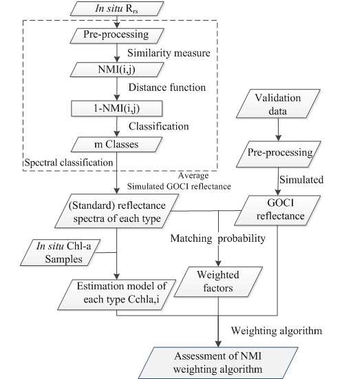
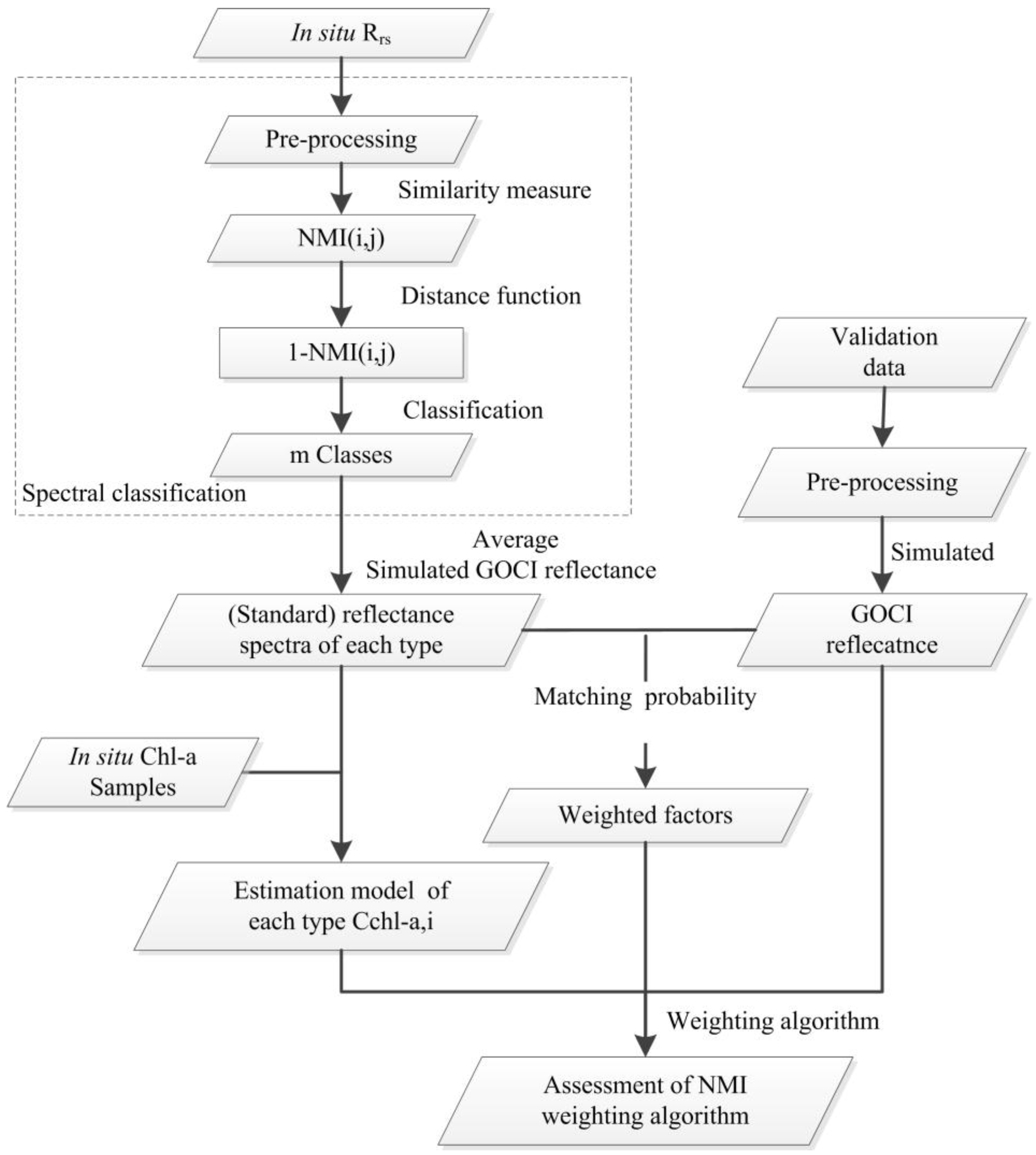
3.2. Spectra Classification and Matching Based on the NMI Algorithm

MI is applied to measure the degree of dependence between two random variables and the information that one variable contains that is found in a second [24]. The basic property of MI is non-negativity, and higher values of MI always indicate dependent variables [21]. NMI is used in this study as the criterion function of the spectral classification and the weighted matching of remote-sensing images. The NMI value between each observed spectrum (or each pixel) and each water type is then assigned as a weighted factor of each Chl-a estimation algorithm.

3.2.1. Normalized Mutual Information Theory

In information theory and Shannon’s entropy theory, A={ak, k=1,..., n} and B={bk, k=1,..., n} are assumed to be two random variables. The MI of the variables can thus be expressed as [23,24]:
I ( A , B ) = H ( B ) H ( B / A )
where H(B) is the marginal entropy of variable B, which describes the uncertainty of variable B; H(B/A) is the conditional entropy, which measures the uncertainty of variable B when variable A is known; and I(A,B) is the MI of A and B:
H ( B ) = b B p B ( b ) log p B ( b )
where p B ( b ) is the marginal probability density of b. The conditional entropy is:
H ( B / A ) = a A b B p A , B ( a , b ) log p A , B ( b / a )
where p A , B ( b ) represents the joint probability density of the variables, and p A , B ( b a ) denotes the conditional probability of variables A and B.
Based on the properties of entropy, the MI of variables A and B can also be expressed by the joint entropy H(A,B) and the probability density function:
I ( A , B ) = H ( A ) + H ( B ) H ( A , B )
I ( A , B ) = a A b B p A , B ( a , b ) log p A , B ( a , b ) p A ( a ) p B ( b )
In addition, two small values of the variable entropies and the independence of variables might lead to small values of MI; thus, an NMI that could avoid the influence of marginal entropies H(A) and H(B) was used as the similarity measure [21]:
N M I = 2 I ( A , B ) H ( A ) + H ( B )

3.2.2. Classification and Matching Algorithms

For the in situ Rrs classification, the NMI values that are used as similarity measurements are first calculated between pairwise normalized Rrs. The NMI value of “0” indicates that the pairwise Rrs is not similar, while the value of “1” represents complete similarity. Therefore, the value of 1-NMI can be applied as a distance function for Rrs classification. Subsequently, the normalized Rrs can be classified into homogeneous types (i.e., Class 1, Class 2, …., Class m) using hierarchical clustering with the distance function D i s ( i , j ) [19].
The equation of the distance function is shown below:
D i s ( i , j ) = 1 N M I ( i , j ) =   1 - 2 I ( R n r s ( i ) , R n r s ( j ) ) H ( R n r s ( i ) ) + H ( R n r s ( j ) )
where D i s ( i , j ) represents the distance function of Rrs; R n r s ( i ) and R n r s ( j ) are the normalized Rrs of i and j; I ( R n r s ( i ) ,   R n r s ( j ) ) is the MI value of R n r s ( i ) ; and H ( R n r s ( i ) ) and H ( R n r s ( j ) ) are the marginal entropies of R n r s ( i ) and R n r s ( j ) .
In addition, the criterion function NMI can also be applied to match the reflectance of the remote-sensing images and the in situ Rrs. However, due to the complex optical properties of inland waters and the fuzzy boundaries between different water types, the observed spectra might not be completely consistent with the standard reflectance spectra of each type. Therefore, a weighted matching method based on NMI was developed in this study. The standard reflectance spectra of each type R n r s , i ¯ ,   i [ 1 , m ] , which represent the average reflectance spectra of each type, can be acquired after classification of the normalized Rrs. To perform the matching algorithm on multi-spectral data, R n r s , i ¯ are first resampled with the spectral response function for the GOCI spectral bands R e   R n r s , i ¯ . The similarity measure between R e   R n r s , i ¯ and the reflectance of the GOCI data S R n r s are then calculated by Equation (9), and the weighted factors of each water type are determined with Equation (10):
S a t N M I ( i ) = 2 I Re R n r s , i ¯ , S R n r s H ( Re R n r s , i ¯ ) + H ( S R n r s )
p N M I ( i ) = S a t N M I ( i ) j = 1 m S a t N M I ( j ) × 100 %
where S a t N M I ( i ) represents the similarity measure between the GOCI data and class i, p N M I ( i ) is the weighted factor (matching probability) for class i, and m is the classification number.

3.3. NMI Weighted Algorithms for Chl-a Estimation

A variety of models based on red and NIR spectral properties have been successfully developed and applied to the estimation of the Chl-a concentration in turbid productive waters [9,11,40]. Considering the spectral bands of GOCI images, a two-band algorithm was used to estimate the Chl-a concentration in inland waters. The two-band relationship between the Chl-a and the NIR-red spectrum can be expressed as [40,41,42]:
C h l - a R r s ( λ 2 ) / R r s ( λ 1 )
where R r s ( λ 1 ) and R r s ( λ 2 ) are the remote-sensing reflectances at wavelengths λ 1 and λ 2 , respectively; and λ 1 is in the red region, in which is approximately the phytoplanktonic absorption peak (660–690 nm), while λ 2 is in the NIR region, where the reflection peaks of phytoplankton (700–730 nm) are typically found. Based on the semi-empirical algorithms and the central wavelengths of the remote sensing images, the corresponding bands of the expressions are bands 5, 6 and 7 for GOCI.
Based on Equation (11), optimum NIR-red models were separately established for each optical type. Therefore, the weighted algorithm for the estimation of Chl-a is given by:
C c h l a = i = 1 m ( p N M I ( i ) × C c h l a , i )
where C c h l a , i is the Chl-a estimated from algorithm i, p N M I ( i ) is the weighted factor (i.e., matching probability) for class i, and m is the classification number.

3.4. Accuracy Assessment

To evaluate the NMI weighted algorithm, the mean absolute error (MAEmean-chla) and the root mean square error (RMSEchla) were calculated as follows:
M A E m e a n c h l a = 1 n i = 1 n | C m e a , i C e s t , i C m e a , i |
R M S E = 1 n i = 1 n ( C m e a , i C e s t , i ) 2
where Cmea,i is the measurement of Cchl-a; Cest,i is the estimated value of Cchl-a; and n is the number of samples.

4. Results

4.1. Variations in the Optical Properties of Each Water Type

After denoising and normalization, samples were classified into three types based on the NMI classification method (Figure 2). Figure 2a–c shows the normalized Rrs of each type; and Figure 2d–e shows the averaged normalized Rrs and the averaged raw Rrs of each type. In combination with Table 2, there were significant differences among the three types based on the spectral shape and the corresponding water parameters.
Compared with Classes 2 and 3, Class 1 waters showed two significant peaks near 562 and 710 nm, and a distinct valley near 675 nm. The reflectance value was higher than the other types in the range of 710 to 900 nm. The difference in the spectral shape was also displayed in bands 6 through 8 in the GOCI data between Class 1 and the other two classes. Class 1 waters showed the highest value of Cchl-a, and the averaged ratio of Cchl-a and CTSM of this class reached 1.95; therefore, Class 1 waters were primarily affected by the Chl-a concentration.
Figure 2. Three types of normalized reflectance spectra based on NMI: (a) Class 1; (b) Class 2; (c) Class 3; (d) average normalized reflectance spectra of each type; (e) average raw reflectance spectra of each type; and (f) normalized spectra resampled to the GOCI bands.
Remotesensing 07 11731 g002
The peak and valley shown in Class 2 were not as significant as those in Class 1 in the NIR range, and the peak of Class 2 was near 700 nm. In this Class, the reflectance value was lower than Class 3 in the range of 400 to 600 nm, while the reflectance value was higher in the range of 600 to 900 nm. The peak around 700 nm in Class 2 was more significantly than that in Class 3. In the GOCI image, the spectral shape of Class 2 was dissimilar to that of Class 1 and Class 3. The slope from bands 6 to 7 in Class 2 was larger than in Class 1. Moreover, the average values of Class 2 from bands 5 to 8 were higher than that of Class 3 and there was a small peak at band 6 in Class 2. Additionally, the average concentration of Chl-a was 22.61 mg/m3, while the average concentration of TSM was 36.31 mg/L; ISM was 29.64 mg/L and aCDOM(440) was 0.51 m−1. The averaged Cchl-a/CTSM ratio of Class 2 was 0.86 and most values of water parameters in Class 2 were between those in Class 1 and Class 3. Therefore, Class 2 was commonly influenced by Chl-a, TSM and CDOM.
Class 3 showed a significant peaks near 565nm in the average normalized reflectance spectra. Compared with Classes 1 and 2, Class 3 did not display the apparent peak or valley in the range of 565 to 900 nm, which was also shown in the GOCI data. The average concentration of Chl-a, TSM and aCDOM(440) in Class 3 was much lower than in Class 1 and Class 2; thus, Class 3 was relatively less affected by Chl-a, TSM and CDOM than the other two classes.
Table 2. Statistical values of water parameters for each type.
Water TypeParameterMinMaxMeanS.D.
Class 1Chl-a(mg/m3)
TSM(mg/L)
ISM(mg/L)
aCDOM(440)(m1)
Chl-a:TSM
21.31
10.50
5.99
0.13
0.46
201.30
86.76
67.31
1.45
6.35
81.63
42.72
19.59
0.61
1.95
42.81
21.09
15.91
0.44
1.66
Class 2Chl-a(mg/m3)
TSM(mg/L)
ISM(mg/L)
aCDOM(440)(m1)
Chl-a:TSM
4.99
12.15
9.00
0.17
0.07
82.65
116.12
106.12
1.89
1.86
22.61
36.31
29.64
0.51
0.86
13.60
18.90
17.29
0.34
0.41
Class 3Chl-a(mg/m3)
TSM(mg/L)
ISM(mg/L)
aCDOM(440)(m1)
Chl-a:TSM
5.29
4.63
2.13
0.16
0.22
36.45
40.34
30.46
1.54
2.57
12.22
8.54
4.67
0.46
1.22
4.71
5.86
3.42
0.38
0.62
Note: S.D. indicates a standard deviation.

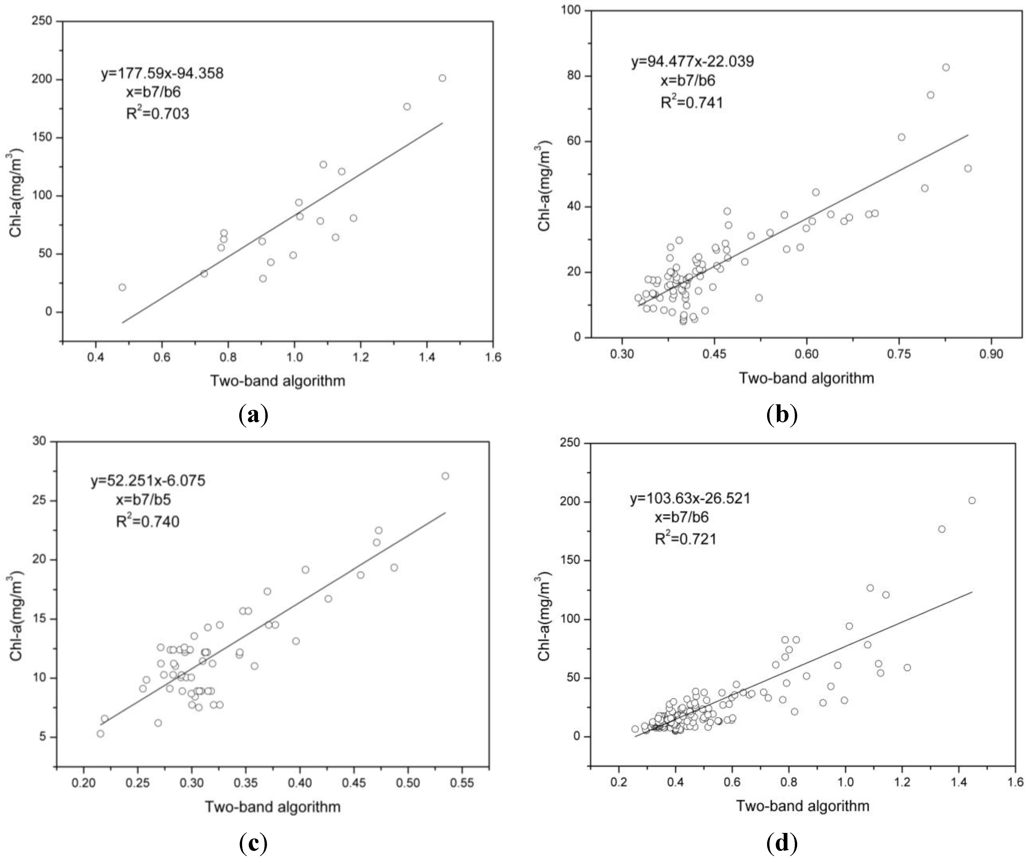
4.2. Estimation of Chl-a Using the NMI Weighted Algorithm

Based on Figure 1, the NIR-red models were first established for the three water types based on Equation (11). The models above, which were directly applied to estimate the Chl-a concentration, were called “hard classification” models in this study. All of the corresponding bands of the GOCI data were applied by the estimation models for each type. Compared to the coefficient of determination R2, the optimum algorithms were separately assigned to each class and unclassified dataset. The results showed that b7/b6 produced better correlation with Chl-a for Class 1, Class 2 and the overall data, while b7/b5 was more suitable for Class 3. Figure 3 shows the models and scatterplot of the Chl-a estimation for the GOCI data.
Subsequently, the simulated GOCI Rnrs (validation data) were applied to calculate the weighted factor ( p N M I ( i ) ), which described the matching probability between the simulated GOCI Rnrs and the standard classified reflectance spectra. Figure 4 shows the matching probabilities of each type for the validation data. The average matching probabilities of Class 1 were 0.20, while the average matching probabilities of Class 2 and Class 3 were 0.42 and 0.38. The results of the matching probabilities indicated that most validation data were difficult to assign to a class; therefore, most samples were dominated by two or three Chl-a estimation models. Finally, the NMI weighted algorithm was applied to estimate the Chl-a using the weighted factors of each type, the NIR-red models for each type and the simulated GOCI Rnrs as input (Equation (12)).

4.3. Validation of the NMI Weighted Algorithm

To evaluate the performance of the NMI weighted algorithm, we compared this method with the non-classification algorithm and hard classification algorithm. The accuracies of the overall validation data and the three types were separately calculated by Equations (13) and (14). Table 3 shows the MAE and RMSE of the above algorithms.
Figure 3. Scatterplot of the Chl-a estimation by the two-band model and the measured Chl-a for GOCI data: (a) Class 1; (b) Class 2; (c) Class 3; and (d) overall data.
Remotesensing 07 11731 g003
Figure 4. Weighted factors of each type for the validation data.
Remotesensing 07 11731 g004
The accuracy of the NMI weighted algorithm with an MAE of 22.63% and an RMSE of 9.41 mg/m3 was generally higher than the results of the other two algorithms; the non-classification algorithm produced an MAE of 31.09% and an RMSE of 12.76 mg/m3, and the hard classification algorithm produced an MAE of 26.23% and an RMSE of 11.02 mg/m3. Thus, the NMI weighted algorithm was acceptable for Chl-a estimation in Taihu Lake. The accuracies of the NMI weighted algorithm for the different classes were also improved. Due to a wide range of Cchl-a values in Class 1 waters, the MAE and RMSE for Class 2 and 3 were better than for Class 1, and the improvement of the RMSE of the NMI weighted algorithm for Class 2 and 3 were relatively smaller than that of Class 1.
Table 3. Comparison of the Chl-a estimation by different algorithms.
GOCI TypeIndexNon-Classification Algorithm Hard-Classification AlgorithmNMI Weighted Algorithm
Class 1MAE
RMSE(mg/m3)
33.4%
28.83
30.06%
25.40
27.28%
22.52
Class 2MAE
RMSE(mg/m3)
28.40%
8.15
25.77%
7.34
21.56%
6.64
Class 3MAE
RMSE(mg/m3)
30.89%
6.67
22.45%
5.98
21.69%
4.37
All validation dataMAE
RMSE(mg/m3)
31.09%
12.76
26.23%
11.02
22.63%
9.41
In addition, Figure 5 shows the scatterplot of the measured Chl-a and the estimated Chl-a in addition to the MAE and RMSE statistics in Table 3. Although the MAE and RMSE of the hard classification algorithm for each water type were higher than that of the non-classification algorithm, the estimated values were shown to exhibit the jumping effect between different water types (Figure 5b). Because different water types could show fuzzy boundaries, similar optical properties might be classified into different types based on the hard classification algorithm, or the observed spectra might not be completely consistent with the specific reflectance spectra of each type [15]. However, the NMI weighted algorithm could reduce this effect (Figure 5c) because the values of Cchl-a were calculated using two or three Chl-a estimation models based on weighted factors. The results indicated that the NMI weighted algorithm not only increased the accuracy of the Chl-a estimation but also avoided the discontinuous or jumping results in different water types.
Figure 5. Scatter plot of the measured and estimated values of Chl-a: (a) non-classification algorithm; (b) hard-classification algorithm; and (c) NMI weighted algorithm.
Remotesensing 07 11731 g005

5. Discussion

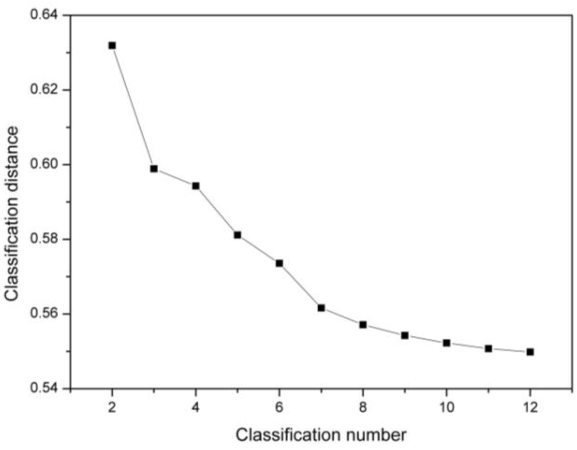
5.1. Assessment of Water Classification

To study the results of the NMI classification, we compared this method to the Ward algorithm, which has been successfully applied for Rrs classification in inland waters [13]. In this study, cophenetic correlation coefficients, which represented the correlation between the clustering information and the distance of original data, were used to evaluate the clustering algorithms [43]. A higher value of the cophenetic correlation coefficient indicated a stronger clustering effect. After calculating the cophenetic correlation coefficient of the NMI classification algorithm and the Ward algorithm, the results showed that the cophenetic correlation coefficient of NMI with the value of 0.8618 was higher than that of the Ward algorithm, which was equal to 0.8056. Combined with Figure 2 and the cophenetic correlation coefficient, the classification algorithm based on NMI was shown to be suitable for Rrs classification, and the classification results produced by the proposed method were better than those of the Ward algorithm in this study.
In addition, the inner-class distance, which was calculated by 1-NMI, was applied to determine the optimum classification number. Because the maximum inner-class distance showed only small variations when the types were greater than 11, Figure 6 shows the relationship between the maximum inner-class distance and the classification number for the water types from 12 to two (12 water types to start with and then two in the end). When the classification number of the water types was from 12 to seven, the values of the distance showed a stable trend. However, the distance changed significantly when the classification number of the water types was less than seven, and the slope between classification number three and two reached a maximum. Therefore, the classification numbers from 12 to seven had no characteristic distinction. In addition, three types were considered as suitable and reasonable results, which also agreed with the water parameters.

5.2. Application of the NMI Weighted Algorithm to GOCI Images

The above studies (Section 4) investigated the potential of the NMI weighting algorithm using GOCI data. Therefore, GOCI images with a spatial resolution of 500 m and a temporal resolution of 1 h were used to analyze the spatial-diurnal distribution of Chl-a in Taihu Lake. Because the images were influenced by scattered clouds at 8:16 a.m., 2:16 p.m. and 3:16 p.m. on 3 September 2011, the remainder of the five images were used to estimate Cchl-a using the NMI weighted algorithm after pre-processing.
Figure 6. Relationship between the classification distance and the classification number.
Remotesensing 07 11731 g006

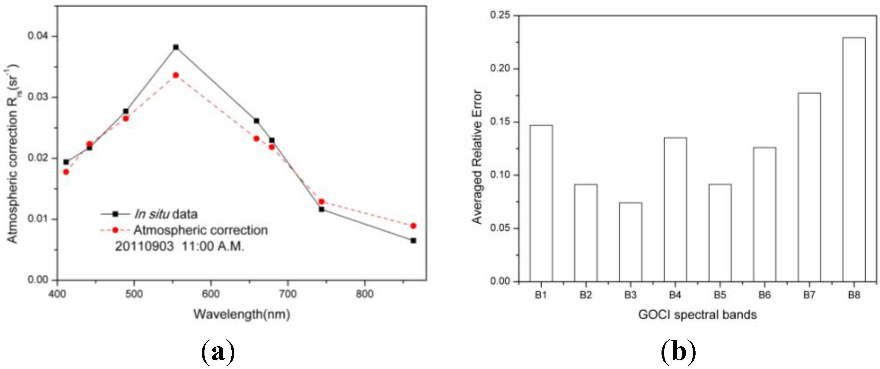
5.2.1. Assessment of Atmospheric Correction

Because the revisit period of the GOCI data is one hour, the 10 samples that were collected closest to the GOCI transit time were used for validation. For each in situ validation dataset, the averaged value of a 3 × 3 pixel window centered at the corresponding location was used for comparison. Figure 7a shows one of the atmospheric correction results of the GOCI data at 11:00 a.m., 3 September 2011. Figure 7b displays the averaged relative error of each band for the GOCI data. The figure shows that the accuracies of bands 2, 3 and 5 with average relative errors of 9.13%, 7.40% and 9.14%, respectively, were higher than other bands. Band 8, with an average relative error of 22.9%, had the lowest accuracy. Bands 5, 6 and 7, which were used to estimate CChl-a, were lower than 18%. The results indicated that the atmospheric correction results could be applied to estimate CChl-a.
Figure 7. Atmospheric correction results of GOCI data: (a) comparison of the in situ data and the atmospheric correction results at 11:00 a.m., 3 September 2011; and (b) statistics of the averaged relative error of each band of the GOCI data.
Remotesensing 07 11731 g007

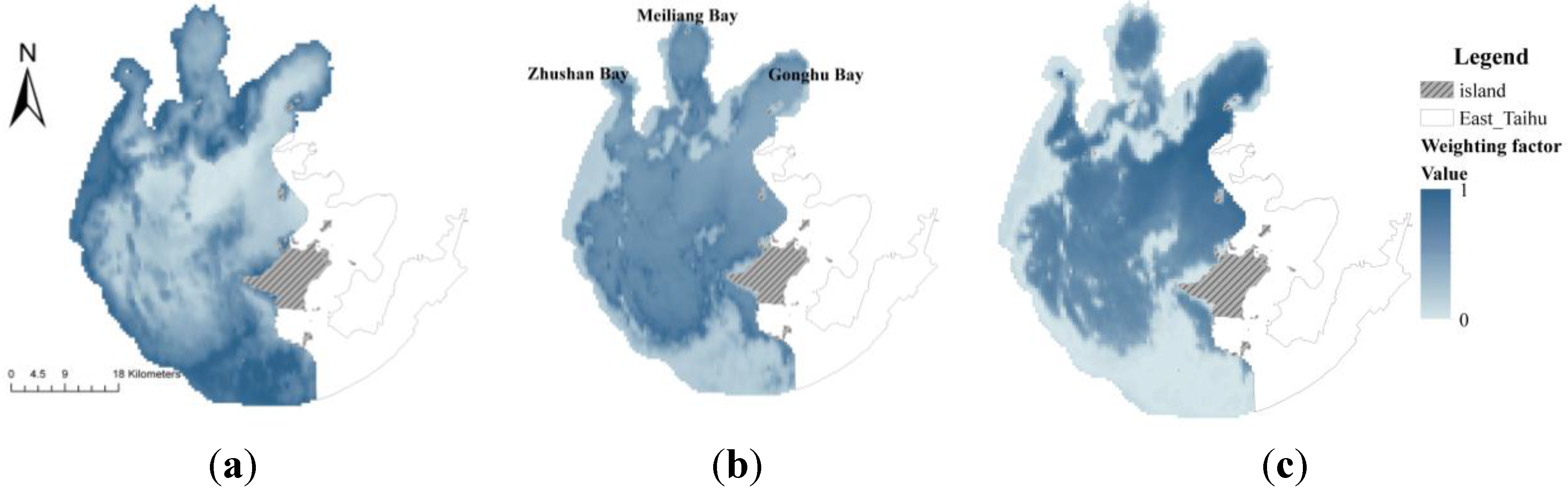
5.2.2. Effect of Fuzzy Boundaries of Water Types in a GOCI Image

Figure 8 shows the weighted-factor images of the GOCI data, which were acquired at 10:16 a.m., 3 September 2011. These images show the degree to which each pixel was classified into each type. For this case, most pixels could not be completely categorized as one type due to the fuzzy boundaries among the different water types present. In the western and southern regions, the weighted factor values of the Class 1 waters were significantly higher than the other two types, while the values of the Class 2 and Class 3 waters played a dominant role in the center of the lake. In Meiliang Bay, the average weighted factors of the three types were all higher than 0.28. Therefore, most regions of Taihu Lake were dominated by two or three Chl-a estimation models in the GOCI image. It was thus feasible to estimate CChl-a for the GOCI images using the NMI weighted algorithm.
Figure 8. Weighting-factor images of each type for GOCI data (10:16 am, 3 September 2011): (a) Class 1; (b) Class 2; and (c) Class 3.
Remotesensing 07 11731 g008

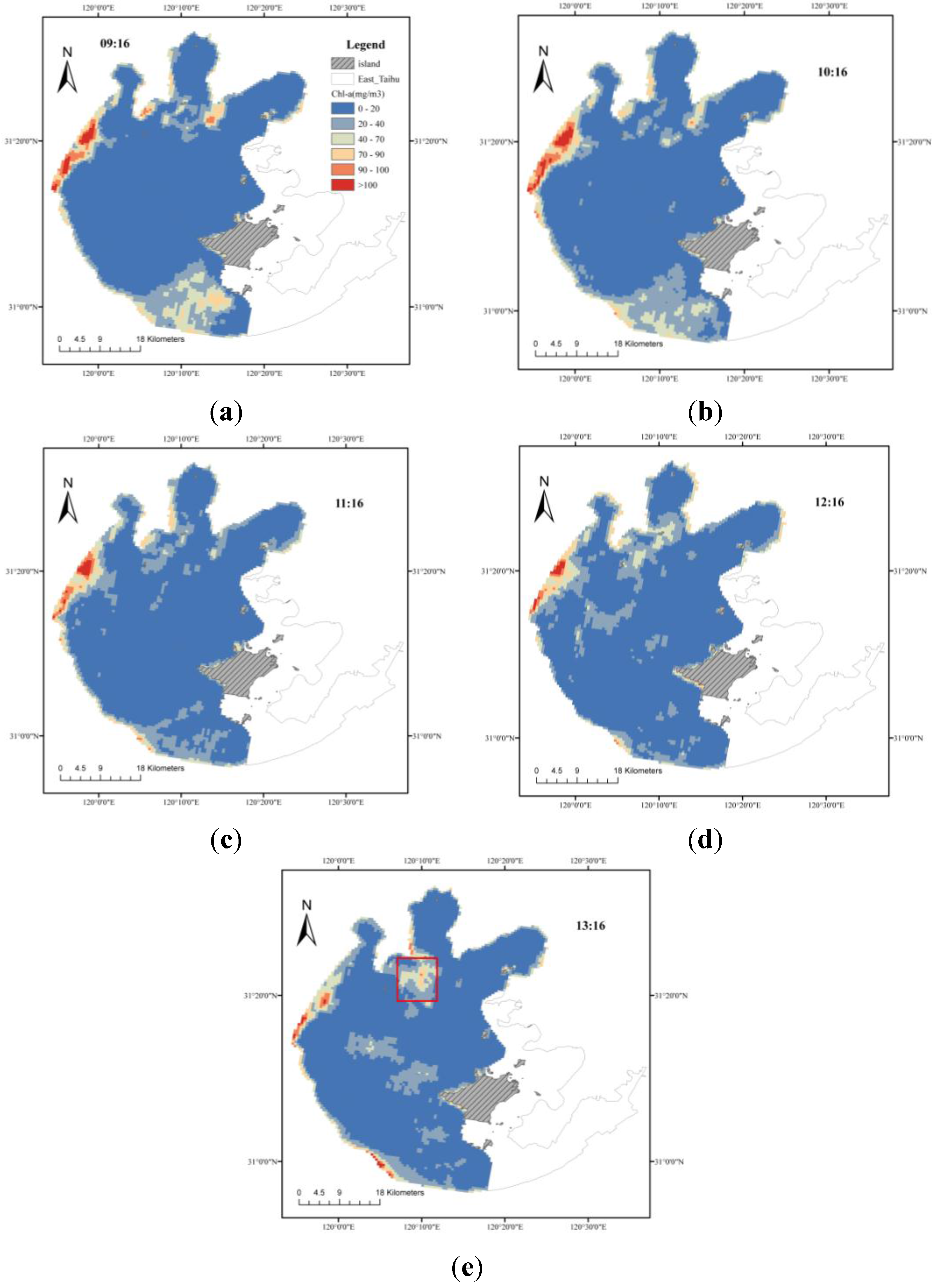
5.2.3. Spatial-Diurnal Distribution of Chl-a in Taihu Lake

Figure 9 shows the spatial and diurnal distribution of Chl-a in Taihu Lake on 3 September 2011. In general, spatial and diurnal differences in Cchl-a existed in Taihu Lake. In the western and southern regions, Cchl-a was significantly higher than in other regions on 3 September 2011. The values of Cchl-a were more than 40 mg/m3 in the western and southern regions of the lake, and some regions were found to exceed 100 mg/m3. However, Cchl-a was found to be distributed between 0 and 20 mg/m3 in other regions (e.g., the center of the lake, Gonghu Bay). The possible reasons for these results were that the runoff entering Taihu Lake was primarily distributed in Meiliang Bay, the western lakeshore and southern lakeshore, and wastewater from farmland, development and industry, which was directly discharged into the lake, provided a growth environment for algae in these regions. In addition, the wind could also bring algae to lakeshore regions [44].
Figure 9. Diurnal distribution of CChl-a on 3 September 2011 (9:16 a.m. to 1:16 p.m.).
Remotesensing 07 11731 g009
The spatial distribution of Cchl-a changed from 9:16 a.m. to 1:16 p.m. In the red rectangular region (Figure 9a) and in the southern lakeshore, high values of Cchl-a were gradually aggregated from 9:16 a.m. to 1:16 p.m.. The values of Cchl-a also increased in the center of the lake from 9:16 a.m. to 1:16 p.m., while the values increased from 9:16 a.m. to 10:16 a.m. and then decreased from 11:16 a.m. to 1:16 p.m. in the western regions. Because Taihu Lake was influenced by northeaster winds during the day, high values of Cchl-a spread to the southwest regions of the lake. Then, the distribution changed in the southern and central regions (i.e., the open area of Taihu Lake). However, the vertical migration of phytoplankton might also have affected the diurnal change of Cchl-a, particularly along the western lakeshore [45,46]. Based on the research of Reynolds [46], blue-green algae could increase at the water surface from early morning to 10:00 a.m. due to the increased buoyancy force of algae cells after photosynthesis. Then, at noon, the algae descended due to the decreased buoyancy force. That study was also applicable to blue-green algae in Xihu Lake, China [47]. Therefore, the diurnal variation along the western lakeshore could be primarily influenced by the vertical migration of blue-green algae because this region had relatively less influence from wind.

6. Conclusions

In this study, the NMI weighted algorithm was proposed to estimate Cchl-a. Based on the in situ normalized reflectance spectra collected from Taihu Lake, three water types were identified by the clustering method, which was implemented by the similarity measure (NMI). Three types had significant differences based on the spectral shape and corresponding water parameters. Class 1 waters showed significant characteristics in the NIR bands and were primarily affected by the Chl-a concentration. Class 2 waters corresponded to the characteristics that were influenced by Chl-a and TSM, while Class 3 waters exhibited lower values of Chl-a and TSS. Based on the three water types, class-specific Chl-a estimation models were developed separately for GOCI data. The weighted factor of each GOCI reflectance was calculated by NMI. Finally, Cchl-a was obtained based on the framework of the NMI weighted algorithm for GOCI data. Compared to the non-classification and the hard-classification algorithms, the NMI weighted algorithm was shown to have a higher accuracy and reduced the discontinuous effect associated with the hard-classification algorithm.
The framework of the NMI weighted algorithm effectively combined class-specific Cchl-a retrievals into a continuous mapping. The method can be applicable to different remote sensing images and Chl-a retrieval algorithms. In the future, the NMI weighted algorithm, which is constructed by other retrieval algorithms such as four-band algorithm [20], normalized difference chlorophyll index [48], and synthetic chlorophyll index [49], will be applied to different satellite images or will be tested in different inland waters. In addition, more in situ data from different regions will be required to completely identify the water types present and to improve the calibrated and validated accuracy.

Acknowledgments

This study was jointly supported by the National Key Technology R&D Program of China (Grant No. 2012BAH32B03), the National Key Basic Research Program Project (Grant No. 2010CB434801), Program B for the Outstanding PhD candidate of Nanjing University (Grant No. 2014001B009), the Scientific Innovation Research of College Graduate in Jangsu Province (Grant No. CXLX12_0040) and the Priority Academic Program Development of Jiangsu Higher Education Institutions (Grant No. 164320H116). The authors would like to thank Yingcheng Lu, Huang Yan, Sun Shaojie and Lin Shan for their valuable suggestions and fieldwork, and would like to thank the Korea Ocean Satellite Center (KOSC) for providing GOCI data. We would also like to thank the anonymous reviewers of this paper for their constructive comments.

Author Contributions

Ying Bao proposed the NMI weighted algorithm and wrote this manuscript. Qingjiu Tian designed the field experiments and participated in the preparation of the manuscript. Min Chen helped to analyze and review the manuscript.

Conflicts of Interest

The authors declare no conflicts of interest.

References

  1. Yang, W.; Matsushita, B.; Chen, J.; Fukushima, T. Estimating constituent concentrations in case II waters from MERIS satellite data by semi-analytical model optimizing and look-up tables. Remote Sens. Environ. 2011, 115, 1247–1259. [Google Scholar] [CrossRef] [Green Version]
  2. Duan, H.; Ma, R.; Hu, C. Evaluation of remote sensing algorithms for cyanobacterial pigment retrievals during spring bloom formation in several lakes of East China. Remote Sens. Environ. 2012, 126, 126–135. [Google Scholar] [CrossRef]
  3. Kutser, T. Quantitative detection of chlorophyll in cyanobacterial blooms by satellite remote sensing. Limnol. Oceanogr. 2004, 49, 2179–2189. [Google Scholar] [CrossRef]
  4. Shi, K.; Li, Y.; Li, L.; Lu, H.; Song, K.; Liu, Z.; Xu, Y.; Li, Z. Remote chlorophyll-a estimates for inland waters based on a cluster-based classification. Sci. Total Environ. 2013, 444, 1–15. [Google Scholar] [CrossRef] [PubMed]
  5. Li, Y.; Wang, Q.; Wu, C.; Zhao, S.; Xu, X.; Wang, Y.; Huang, C. Estimation of chlorophyll a concentration using NIR/red bands of MERIS and classification procedure in inland turbid water. IEEE Trans. Geosci. Remote Sens. 2012, 50, 988–997. [Google Scholar] [CrossRef]
  6. Song, K.; Li, L.; Tedesco, L.P.; Li, S.; Duan, H.; Liu, D.; Hall, B.E.; Du, J.; Li, Z.; Shi, K.; et al. Remote estimation of chlorophyll-a in turbid inland waters: Three-band model versus GA-PLS model. Remote Sens. Environ. 2013, 136, 342–357. [Google Scholar] [CrossRef]
  7. Yu, G.; Yang, W.; Matsushita, B.; Li, R.; Oyama, Y.; Fukushima, T. Remote estimation of chlorophyll-a in inland waters by a NIR-red-based algorithm: Validation in Asian Lakes. Remote Sens. 2014, 6, 3492–3510. [Google Scholar] [CrossRef] [Green Version]
  8. Huang, C.; Zou, J.; Li, Y.; Yang, H.; Shi, K.; Li, J.; Wang, Y.; Chena, X.; Zheng, F. Assessment of NIR-red algorithms for observation of chlorophyll-a in highly turbid inland waters in China. ISPRS J. Photogramm. Remote Sens. 2014, 93, 29–39. [Google Scholar] [CrossRef]
  9. Dall’Olmo, G.; Gitelson, A.A.; Rundquist, D.C.; Leavitt, B.; Barrow, T.; Holz, J.C. Assessing the potential of SeaWiFS and MODIS for estimating chlorophyll concentration in turbid productive waters using red and near-infrared bands. Remote Sens. Environ. 2005, 96, 176–187. [Google Scholar] [CrossRef]
  10. Moses, W.J.; Gitelson, A.A.; Povazhnyy, V. Estimation of chlorophyll-a concentration in case II waters using MODIS and MERIS data—Successes and challenges. Environ. Res. Lett. 2009, 4. [Google Scholar] [CrossRef]
  11. Le, C.; Hu, C.; Cannizzaro, J.; English, D.; Muller-Karger, F.; Lee, Z. Evaluation of chlorophyll-a remote sensing algorithms for an optically complex estuary. Remote Sens. Environ. 2013, 129, 75–89. [Google Scholar] [CrossRef]
  12. Zhang, Y.; Lin, H.; Chen, C.; Chen, L.; Zhang, B.; Gitelson, A.A. Estimation of chlorophyll-a concentration in estuarine waters: Case study of the Pearl River estuary, South China Sea. Environ. Res. Lett. 2011, 6. [Google Scholar] [CrossRef]
  13. Vantrepotte, V.; Loisel, H.; Dessailly, D.; Meriaux, X. Optical classification of contrasted coastal waters. Remote Sens. Environ. 2012, 123, 306–323. [Google Scholar] [CrossRef]
  14. El-Alem, A.; Chokmani, K.; Laurion, I.; El-Adloini, S.E. An adaptive model to monitor chlorophyll-a in inland waters in southern Quebec using downscaled MODIS imagery. Remote Sens. 2014, 6, 6446–6471. [Google Scholar] [CrossRef]
  15. Moore, T.S.; Dowell, M.D.; Bradt, S.; Verdu, A.R. An optical water type framework for selecting and blending retrievals from bio-optical algorithms in lakes and coastal waters. Remote Sens. Environ. 2014, 143, 97–111. [Google Scholar] [CrossRef] [PubMed]
  16. Moore, T.S.; Campbell, J.W.; Feng, H. A fuzzy logic classification scheme for selecting and blending satellite ocean color algorithms. IEEE Trans. Geosci. Remote Sens. 2001, 39, 1764–1776. [Google Scholar] [CrossRef]
  17. Lyu, H.; Zhang, J.; Zha, G.; Wang, Q.; Li, Y. Developing a two-step retrieval method for estimating total suspended solid concentration in Chinese turbid inland lakes using Geostationary Ocean Colour Imager (GOCI) imagery. Int. J. Remote Sens. 2015, 36, 1385–1405. [Google Scholar] [CrossRef]
  18. Le, C.F.; Li, Y.; Zha, Y.; Sun, D.; Huang, C.; Zhang, H. Remote estimation of chlorophyll a in optically complex waters based on optical classification. Remote Sens. Environ. 2011, 115, 725–737. [Google Scholar] [CrossRef]
  19. Lubac, B.; Loisel, H. Variability and classification of remote sensing reflectance spectra in the eastern English Channel and southern North Sea. Remote Sens. Environ. 2007, 110, 45–58. [Google Scholar] [CrossRef]
  20. Zhang, F.; Li, J.; Shen, Q.; Zhang, B.; Wu, C.; Wu, Y.; Wang, G.; Wang, S.; Lu, Z. Algorithms and schemes for chlorophyll a estimation by remote sensing and optical classification for Turbid Lake Taihu, China. IEEE J. Sel. Top. Appl. Earth Obs. Remote Sens. 2014, 8, 350–364. [Google Scholar] [CrossRef]
  21. Martínez-Usó, A.; Pla, F.; Sotoca, J.M.; Garcia-Sevilla, P. Clustering-based hyperspectral band selection using information measures. IEEE Trans. Geosci. Remote Sens. 2007, 45, 4158–4171. [Google Scholar] [CrossRef]
  22. Bao, Y.; Tian, Q.; Chen, M.; Lin, H. An automatic extraction method for individual tree crowns based on self-adaptive mutual information and tile computing. Int. J. Digital Earth 2015, 8, 495–516. [Google Scholar] [CrossRef]
  23. Del Moral, F.G.; Guillen, A.; Del Moral, L.G.; O’Valle, F.; Martinez, L.; Del Moral, R.G. Duroc and Iberian pork neural network classification by visible and near infrared reflectance spectroscopy. J. Food Eng. 2009, 90, 540–547. [Google Scholar] [CrossRef]
  24. Long, X.X.; Li, H.D.; Fan, W.; Xu, Q.S.; Liang, Y.Z. A model population analysis method for variable selection based on mutual information. Chemom. Intell. Lab. Syst. 2012, 121, 75–81. [Google Scholar] [CrossRef]
  25. Ma, R.; Dai, J. Investigation of chlorophyll-a and total suspended matter concentrations using Landsat ETM and field spectral measurement in Taihu Lake, China. Int. J. Remote Sens. 2005, 26, 2779–2795. [Google Scholar] [CrossRef]
  26. Zhao, D.; Cai, Y.; Jiang, H.; Xu, D.; Zhang, W.; An, S. Estimation of water clarity in Taihu Lake and surrounding rivers using Landsat imagery. Adv. Water Resour. 2011, 34, 165–173. [Google Scholar] [CrossRef]
  27. Jiao, H.B.; Zha, Y.; Gao, J.; Li, Y.M.; Wei, Y.C.; huang, J.Z. Estimation of chlorophyll-a concentration in Lake Tai, China using in situ hyperspectral data. Int. J. Remote Sens. 2006, 27, 4267–4276. [Google Scholar] [CrossRef]
  28. Mobley, C.D. Estimation of the remote-sensing reflectance from above-surface measurements. Appl. Opt. 1999, 38, 7442–7455. [Google Scholar] [CrossRef] [PubMed]
  29. Tang, J.W.; Tian, G.L.; Wang, X.Y.; Wang, X.M.; Song, Q.J. Methods of water spectra measurement and analysis I: Above-water method. J. Remote Sens. 2004, 8, 37–44. [Google Scholar]
  30. Lorenzen, C. Determination of chlorophyll and pheo-pigments: Spectrophotometric equations. Limnol. Oceanogr. 1967, 2, 343–346. [Google Scholar] [CrossRef]
  31. Moses, W.J.; Gitelson, A.A.; Berdnikov, S.; Saprygin, V.; Povazhnyi, V. Operational MERIS-based NIR-red algorithms for estimating chlorophyll-a concentrations in coastal waters—The Azov Sea case study. Remote Sens. Environ. 2012, 121, 118–124. [Google Scholar] [CrossRef]
  32. Wang, Q. Mechanisms of remote-sensing reflectance variability and its relation to bio-optical processes in a highly turbid eutrophic lake: Lake Taihu (China). IEEE Trans. Geosci. Remote Sens. 2010, 48, 575–584. [Google Scholar] [CrossRef]
  33. Korea Ocean Satellite Center (KOSC). Available online: http://kosc.kordi.re.kr/ (accessed on 10 September 2015).
  34. Duan, H.; Ma, R.; Zhang, Y.; Loiselle, S.A.; Xu, J.; Zhao, C.; Zhou, L.; Shang, L. A new three-band algorithm for estimating chlorophyll concentrations in turbid inland lakes. Environ. Res. Lett. 2010, 5. [Google Scholar] [CrossRef]
  35. Wang, M.; Shi, W.; Jiang, L. Atmospheric correction using near-infrared bands for satellite ocean color data processing in the turbid western Pacific region. Opt. Express 2012, 20, 741–753. [Google Scholar] [CrossRef] [PubMed]
  36. Zhang, J.; Yuan, L.; Pu, R.; Loraamm, R.W.; Yang, G.; Wang, J. Comparison between wavelet spectral features and conventional spectral features in detecting yellow rust for winter wheat. Comput. Electron. Agric. 2014, 100, 79–87. [Google Scholar] [CrossRef]
  37. Liew, S.C.; Lin, I.I.; Kwoh, L.K.; Holmes, M.; Teo, S.; Gin, K.; Lim, H. Spectral Reflectance Signatures of Case II Waters: Potential for Tropical Algal Bloom Monitoring Using Satellite Ocean Color Sensors. In Proceddings of 10th JSPS/VCC Joint Seminar on Marine and Fisheries Sciences, Melaka, Malaysia, 29 November–1 December 1999.
  38. Liang, L.; Wang, B.; Guo, Y.; Ni, H.; Ren, Y. A support vector machine-based analysis method with wavelet denoised near-infrared spectroscopy. Vib. Spectrosc. 2009, 49, 274–277. [Google Scholar] [CrossRef]
  39. Wu, C. Normalized spectral mixture analysis for monitoring urban composition using ETM+ imagery. Remote Sens. Environ. 2004, 93, 480–492. [Google Scholar] [CrossRef]
  40. Gitelson, A.A.; Dall’Olmo, G.; Moses, W.; Rundquist, D.C.; Barrow, T.; Fisher, T.R.; Gurlin, D.; Holz, J. A simple semi-analytical model for remote estimation of chlorophyll-a in turbid waters: Validation. Remote Sens. Environ. 2008, 112, 3582–3593. [Google Scholar] [CrossRef]
  41. Gitelson, A. The peak near 700 nm on radiance spectra of algae and water: Relationships of its magnitude and position with chlorophyll concentration. Int. J. Remote Sens. 1992, 13, 3367–3373. [Google Scholar] [CrossRef]
  42. Ruddick, K.G.; Gons, H.J.; Rijkeboer, M.; Tilstone, G. Optical remote sensing of chlorophyll a in case 2 waters by use of an adaptive two-band algorithm with optimal error properties. Appl. Opt. 2001, 40, 3575–3585. [Google Scholar] [CrossRef] [PubMed]
  43. Saraçli, S.; Doğan, N.; Doğan, I. Comparison of hierarchical cluster analysis methods by cophenetic correlation. J. Inequal. Appl. 2013, 2013, 1–8. [Google Scholar] [CrossRef]
  44. Zhang, Y.L.; Qin, B.Q.; Liu, M.L. Temporal-spatial variations of chlorophyll a and primary production in Meiliang Bay, Lake Taihu, China from 1995 to 2003. J. Plankton Res. 2007, 29, 707–719. [Google Scholar] [CrossRef]
  45. Lou, X.; Hu, C. Diurnal changes of a harmful algal bloom in the East China Sea: Observations from GOCI. Remote Sens. Environ. 2014, 140, 562–572. [Google Scholar] [CrossRef]
  46. Reynolds, C.S.; Walsby, A.E. Water blooms. Biol. Rev. 1975, 50, 437–481. [Google Scholar] [CrossRef]
  47. Xiang, S.; Lu, G. The diurnal rhythm of phytoplankton in an eutrophic lake-West Lake, Hangzhou. Acta Hydrob. Sin. 1992, 16, 125–132. [Google Scholar]
  48. Mishra, S.; Mishra, D.R. Normalized difference chlorophyll index: A novel model for remote estimation of chlorophyll-a concentration in turbid productive waters. Remote Sens. Environ 2012, 117, 394–406. [Google Scholar] [CrossRef]
  49. Shen, F.; Zhou, Y.; Li, D.; Zhu, W.; Suhyb Salama, M. Medium resolution imaging spectrometer (MERIS) estimation of chlorophyll-a concentration in the turbid sediment-laden waters of the Changjiang (Yangtze) Estuary. Int. J. Remote Sens. 2010, 31, 4635–4650. [Google Scholar] [CrossRef]

