Seafloor Sediment Study from South China Sea: Acoustic & Physical Property Relationship

Abstract
:
1. Introduction
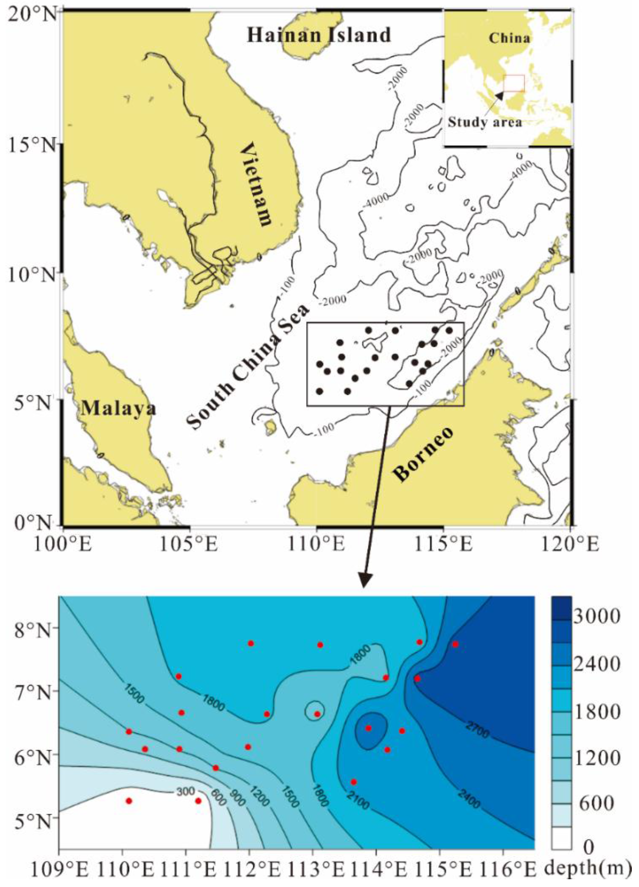
2. Study Area

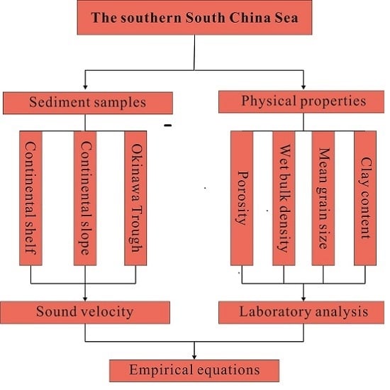
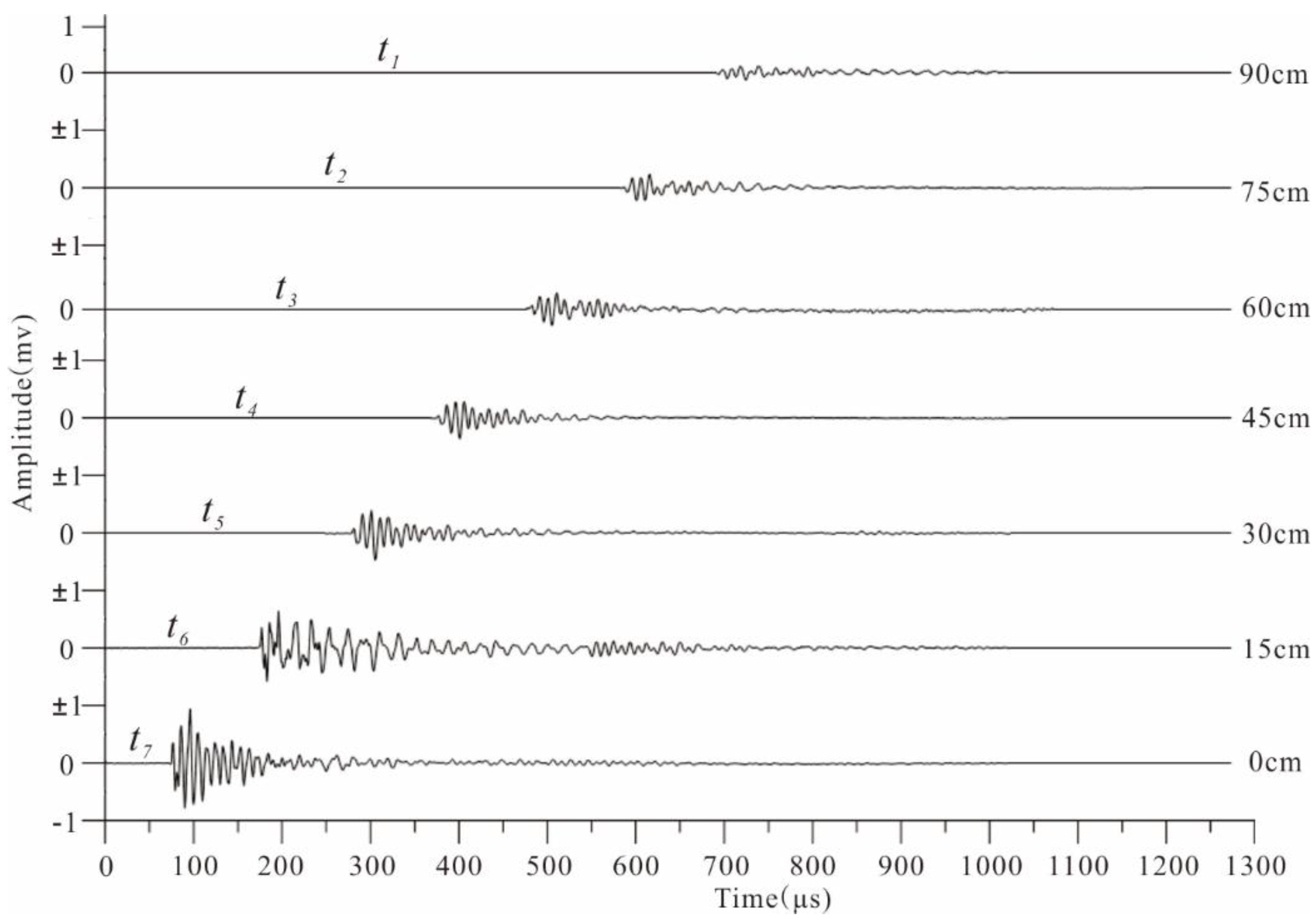
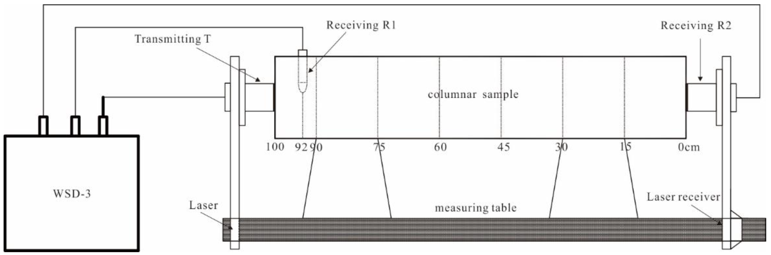
3. Methods

- (1)
- The intact cylindrical sample within the polyethylene core liner was placed on the measuring table immediately upon retrieval.
- (2)
- The WSD-3 transducers were connected to the sediment core.
- (a)
- The receiving transducer R1 was inserted into the sediment core at the position of 92 cm.
- (b)
- The transmitting transducer T was pressed firmly against the sediment core at the bottom of the core (at the position of 100 cm).
- (c)
- The receiving transducer R2 was pressed firmly against the sediment core at the bottom of the core (at the position of 0 cm).
4. Results and Discussion
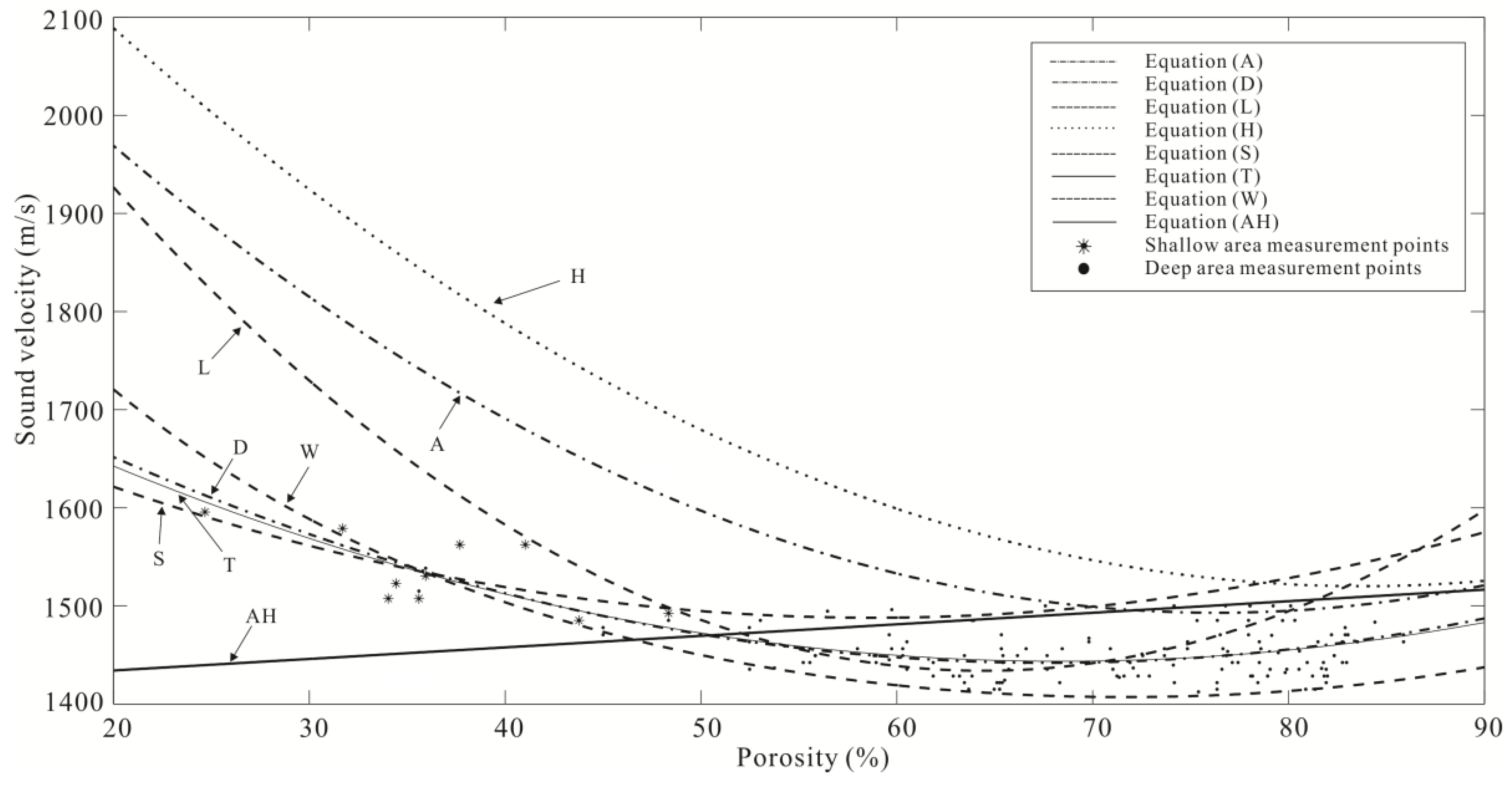
4.1. Porosity
- Equation (H): Hamilton & Bachman (H), V = 2502.0 − 23.45n + 0.14n2
- Equation (AH): Hamilton & Bachman abyssal hill (AH), V = 1410.6 − 1.177n
- Equation (A): Anderson (A), V = 2506 − 27.58n + 0.1868n2
- Equation (L): Lu et al. (L), V = 2470.7 − 32.2n + 0.25n2
- Equation (T): The entire study area (T), V = 1841 − 11.62n + 0.08493n2
- Equation (S): The shallow zone (S), V = 1795 − 10.46n + 0.08907n2
- Equation (D): The deep zone (D), V = 1864 − 12.45n + 0.09182n2


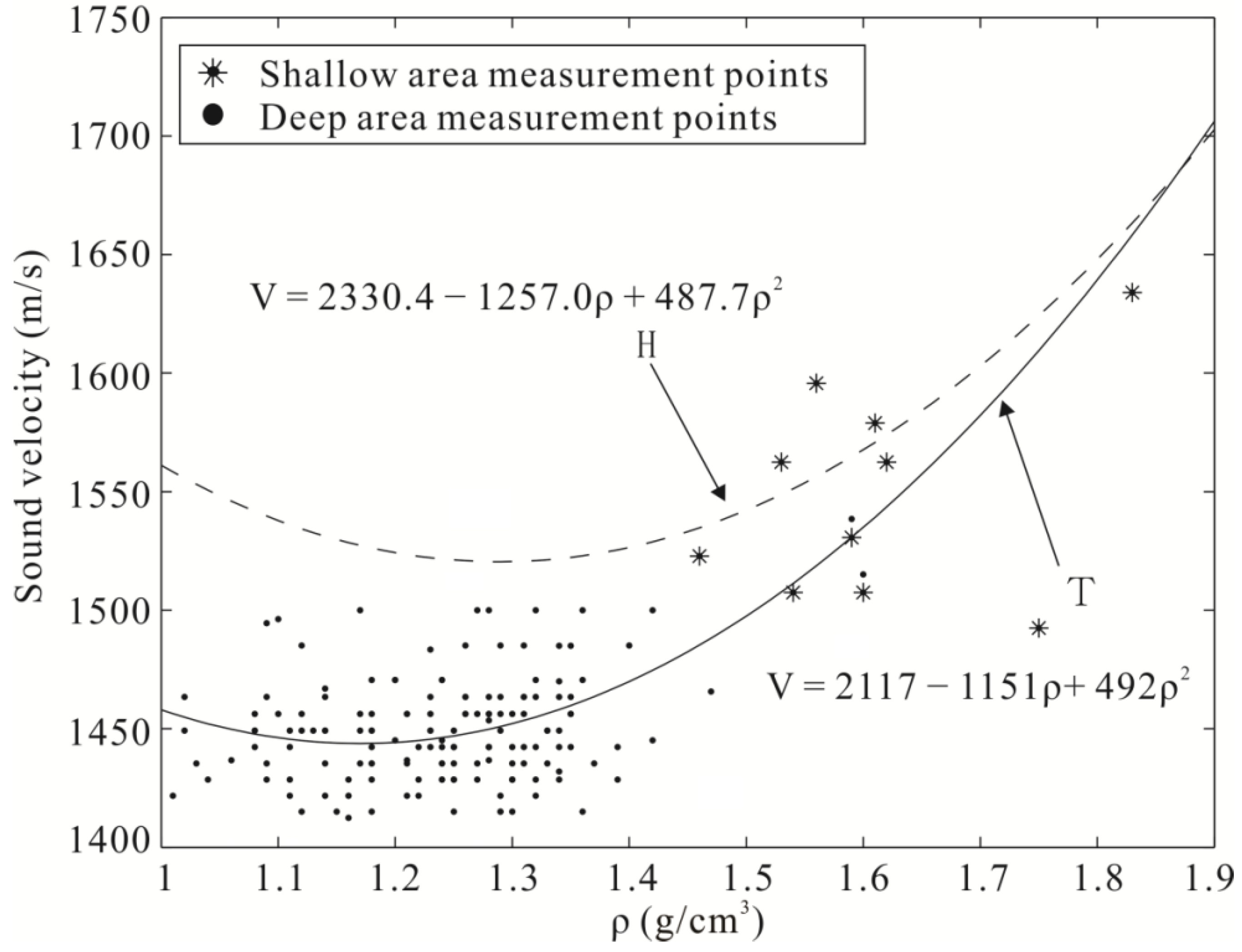
4.2. Wet Bulk Density
- Equation (H): Hamilton & Bachman (H), V = 2330.4 − 1257.0ρ + 487.7ρ2
- Equation (T): The entire study area (T), V = 2117 − 1151ρ + 492ρ2

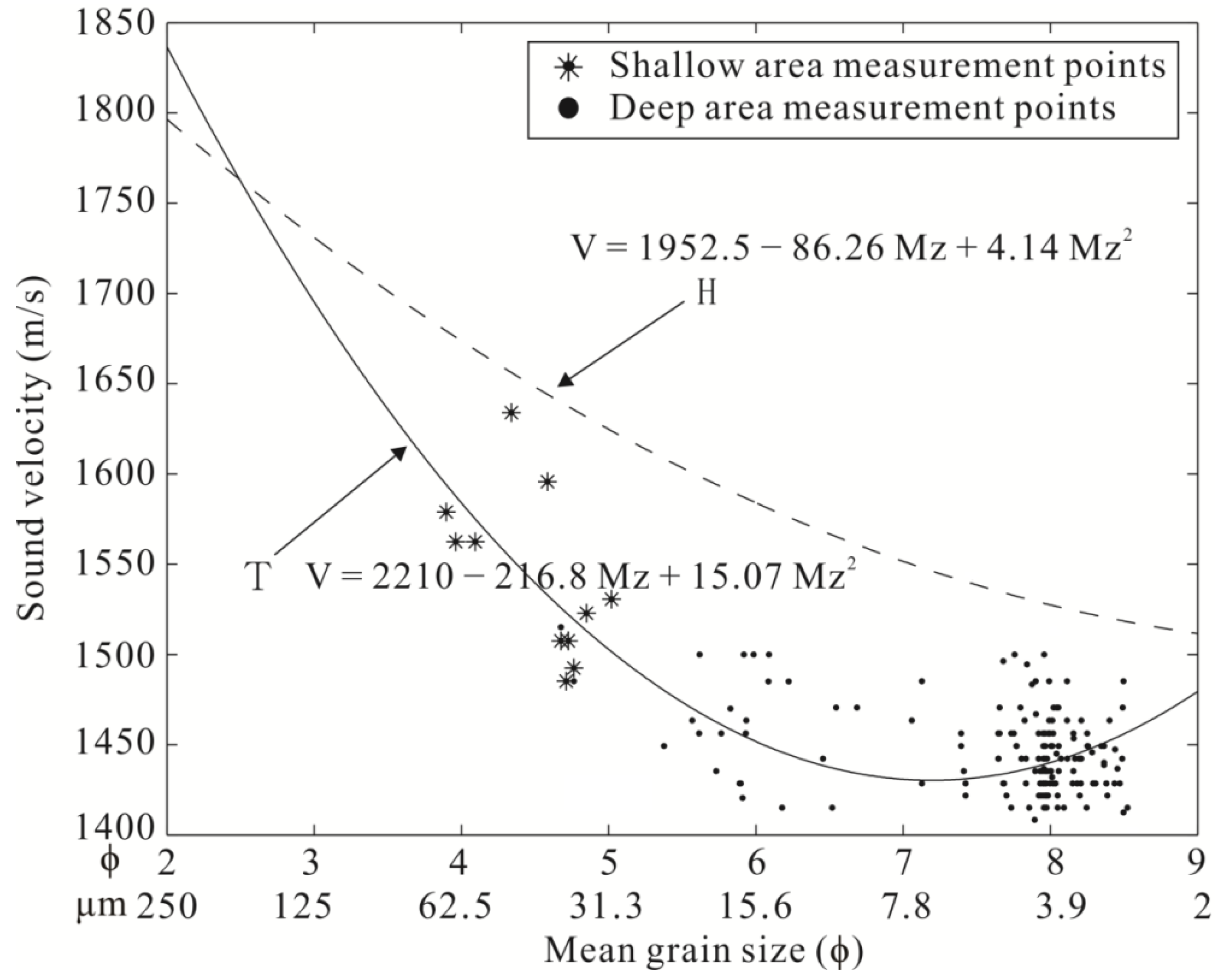
4.3. Mean Grain Size
- Equation (H): Hamilton & Bachman (H), V = 1952.5 − 86.26 Mz + 4.14 Mz2
- Equation (T): The entire study area (T), V = 2210 − 216.8 Mz + 15.07 Mz2

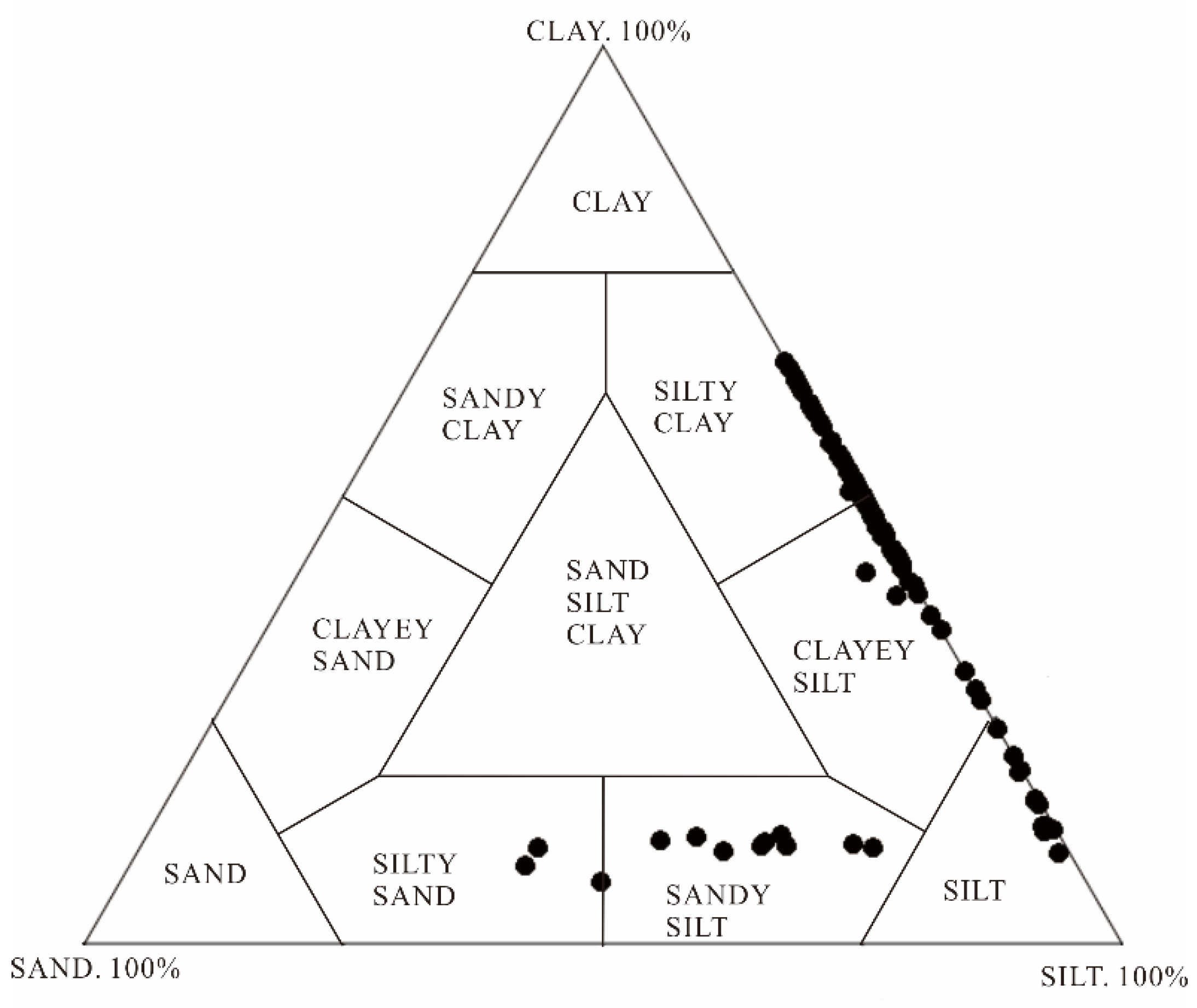
| Geographical Area | Type | Water Depth (m) | Velocity (m/s) | Sand (%) | Silt (%) | Clay (%) | |
|---|---|---|---|---|---|---|---|
| Shallow areas | Continental shelf | Mean | 142 | 1533.47 | 34.02 | 55.37 | 10.61 |
| Max | 148 | 1595.74 | 53.04 | 70.73 | 12.06 | ||
| Min | 136 | 1485.15 | 18.53 | 38.16 | 6.86 | ||
| Deepareas | Continental slope | Mean | 1605 | 1447.14 | 0.20 | 54.39 | 45.41 |
| Max | 2028 | 1543.21 | 3.96 | 86.18 | 57.63 | ||
| Min | 1053 | 1415.10 | 0.00 | 42.37 | 12.53 | ||
| Trough | Mean | 2521 | 1448.83 | 0.15 | 51.98 | 47.87 | |
| Max | 2843 | 1500.00 | 1.12 | 88.86 | 64.92 | ||
| Min | 2207 | 1412.43 | 0.00 | 35.08 | 10.02 | ||
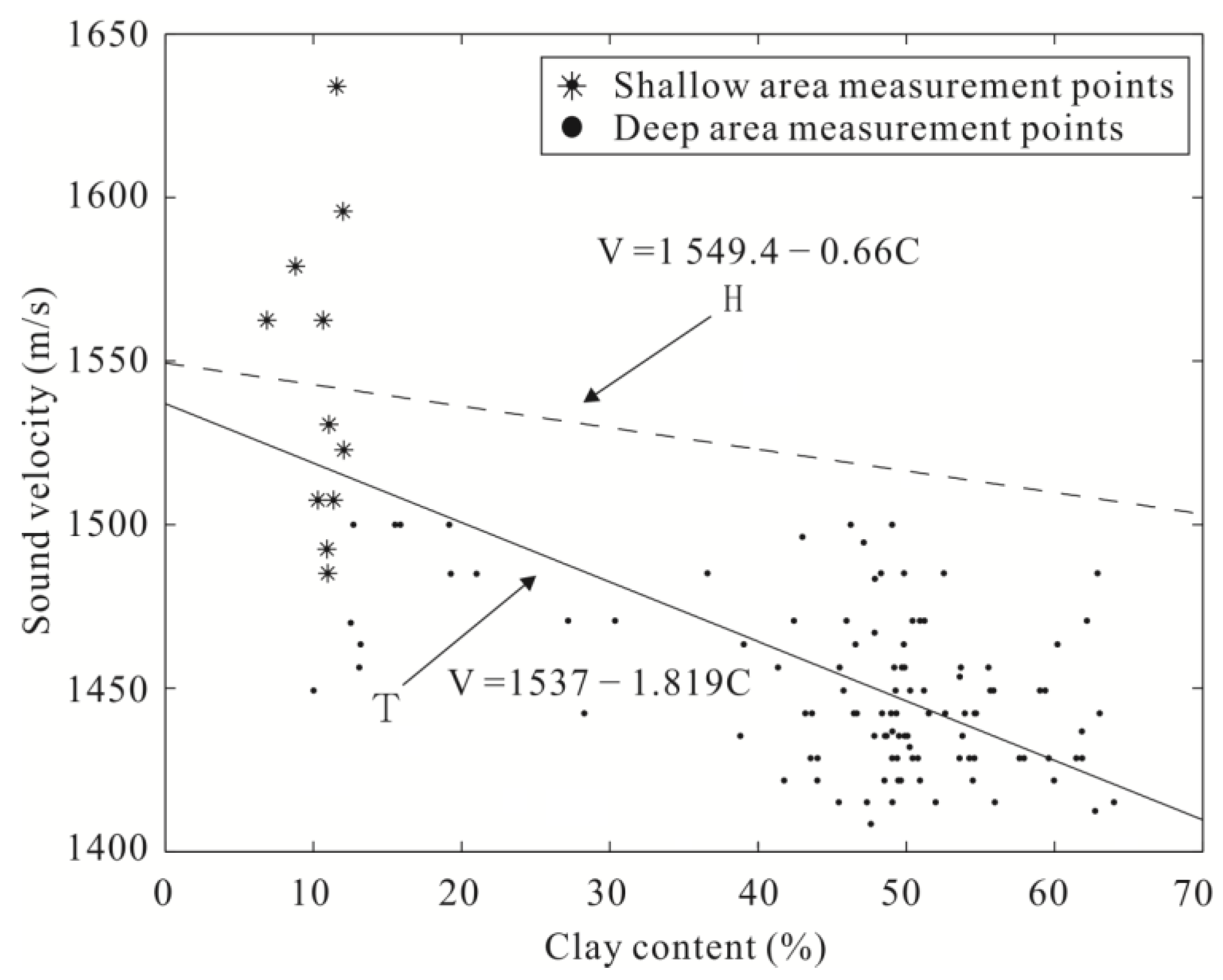
4.4. Clay Content
- Equation (H): Hamilton & Bachman (H), V = 1549.4 − 0.66C
- Equation (T): The entire study area (T), V = 1537 − 1.819C
4.5. Sound Velocity

5. Conclusions
- (1)
- Previously established equations relating the physical properties of seafloor sediment to their acoustic properties were not entirely accurate in the study area.
- (2)
- We developed new empirical equations describing the relationships of the physical and acoustic properties of the samples, corresponding to the different geographical areas in our study area. Comparing the results of the new equations and the previous ones and analyzing the factors influencing the discrepancies between the results indicates that the physical properties, sediment types, geographical areas, and sand-silt-clay ratios are important factors affecting sound velocity in sediment.
- (3)
- Future work in this field should include experimental and theoretical exploration of the influence of various potential impacting factors, and use of more discriminating acoustic techniques (such as in situ measurement).
Acknowledgments
Author Contributions
Conflicts of Interest
References
- Gorgas, T.J.; Wilkens, R.H.; Fu, S.S.; Frazer, L.N.; Richardson, M.D.; Briggs, K.B.; Lee, H. In situ acoustic and laboratory ultrasonic sound speed and attenuation measured in heterogeneous soft seabed sediments: Eel River shelf, California. Mar. Geol. 2002, 182, 103–119. [Google Scholar] [CrossRef]
- Biot, M.A. Theory of propagation of elastic waves in a fluid-saturated porous solid. I. Low frequency range. J. Acoust. Soc. Am. 1956, 28, 168–178. [Google Scholar] [CrossRef]
- Biot, M.A. Theory of propagation of elastic waves in a fluid-saturated porous solid. II. Higher frequency range. J. Acoust. Soc. Am. 1956, 28, 179–191. [Google Scholar] [CrossRef]
- Stoll, R.D. Marine sediment acoustics. J. Acoust. Soc. Am. 1985, 77, 1789–1799. [Google Scholar] [CrossRef]
- Hamilton, E.L. Sound velocity and related properties of marine sediments, North Pacific. J. Geophys. Res. 1970, 75, 4423–4446. [Google Scholar] [CrossRef]
- Hamilton, E.L. Elastic properties of marine sediments. J. Geophys. Res. 1971, 76, 579–603. [Google Scholar] [CrossRef]
- Hamilton, E.L. Geoacoustic modeling of the sea floor. J. Acoust. Soc. Am. 1980, 68, 1313–1340. [Google Scholar] [CrossRef]
- Hamilton, E.L.; Bachman, R.T. Sound velocity and related properties of marine sediments. J. Acoust. Soc. Am. 1982, 72, 1891–1904. [Google Scholar] [CrossRef]
- Orsi, T.H.; Dunn, D.A. Sound velocity and related physical properties of fine grained abyssal sediments from the Brazil Basin (South Atlantic Ocean). J. Acoust. Soc. Am. 1990, 88, 1536–1542. [Google Scholar] [CrossRef]
- Brandes, H.G.; Silva, A.J.; Walter, D.J. Geo-acoustic characterization of calcareous seabed in the Florida Keys. Mar. Geol. 2002, 182, 77–102. [Google Scholar] [CrossRef]
- Lambert, D.N.; Kalcic, M.T.; Faas, R.W. Variability in the acoustic response of shallow-water marine sediments determined by normal-incident 30-kHz and 50-kHz sound. Mar. Geol. 2002, 182, 179–208. [Google Scholar] [CrossRef]
- Briggs, K.B.; Richardson, M.D. Small-scale fluctuations in acoustic and physical properties in surficial carbonate sediments and their relationship to bioturbation. Geo-Mar. Lett. 1997, 17, 306–315. [Google Scholar] [CrossRef]
- Richardson, M.D.; Briggs, K.B.; Bentley, S.J.; Walter, D.J.; Orsi, T.H. The effects of biological and hydrodynamic processes on physical and acoustic properties of sediments off the Eel River, California. Mar. Geol. 2002, 182, 121–139. [Google Scholar] [CrossRef]
- Kim, G.Y.; Kim, D.C.; Yoo, D.G.; Shin, B.K. Physical and Geoacoustic properties of surface sediments off eastern Geoje Island, South Sea of Korea. Quat. Int. 2001, 230, 21–33. [Google Scholar] [CrossRef]
- Jackson, D.; Richardson, M. Geoacoustic properties. In High-Frequency Seafloor Acoustics; Springer Science & Business Media: Berlin, Germany, 2007; pp. 123–170. [Google Scholar]
- Lu, B.; Li, G.; Sun, D.; Huang, S.; Zhang, F. Acoustic-physical properties of seafloor sediments from near shore southeast China and their correlations. J. Tropi. Oceanogr. 2006, 25, 12–17. (In Chinese) [Google Scholar]
- Lu, B.; Li, G.; Liu, Q.; Huang, S.; Zhang, F. Sea floor sediment and its acoustic-physical properties in the southeast open sea area of Hainan Island in China. Mar. Georesources Geotechnol. 2008, 26, 129–144. [Google Scholar] [CrossRef]
- Kan, G.; Liu, B.; Zhao, Y.; Li, G.; Pei, Y. Self-contained in situ sediment acoustic measurement system based on hydraulic driving penetration. High Technol. Lett. 2011, 17, 311–316. [Google Scholar]
- Liu, B.; Han, T.; Kan, G.; Li, G. Correlations between the in situ acoustic properties and geotechnical parameters of sediments in the Yellow Sea, China. J. Asian Earth Sci. 2013, 77, 83–90. [Google Scholar] [CrossRef]
- Kim, D.C.; Sung, J.Y.; Park, S.C.; Lee, G.H.; Choi, J.H.; Kim, G.Y.; Kim, J.C. Physical and acoustic properties of shelf sediments, the South Sea of Korea. Mar. Geol. 2011, 179, 39–50. [Google Scholar] [CrossRef]
- Anderson, R.S. Statistical correlation of physical properties and sound velocity in sediments. In Physics of Sound in Marine Sediments; Hampton, L., Ed.; Plenum Press: New York, NY, USA, 1974; pp. 481–518. [Google Scholar]
- Bachman, R.T. Acoustic and physical property relationships in marine sediment. J. Acoust. Soc. Am. 1985, 78, 616–621. [Google Scholar] [CrossRef]
- Han, D.; Nur, A.; Morgan, D. Effects of porosity and clay content on wave velocities in sandstones. Geophysics 1986, 51, 2093–2107. [Google Scholar] [CrossRef]
- Neto, A.A.; Teixeira Mendes, J.D.N.; de Souza, J.M.G.; Redusino, M., Jr.; Leandro Bastos Pontes, R. Geotechnical influence on the acoustic properties of marine sediments of the Santos Basin, Brazil. Mar. Georesources Geotechnol. 2013, 31, 125–136. [Google Scholar] [CrossRef]
- Horn, D.R.; Horn, B.M.; Delach, M.N. Correlation between acoustical and other physical properties of deep-sea cores. J. Geophys. Res. 1968, 73, 1939–1957. [Google Scholar] [CrossRef]
- Kumar, T.P. A Study on the Geoacoustics Properties of the Marine Sediments. PhD Thesis, Cochin University Science & Technology, Cochin, India, December 1999. [Google Scholar]
- Chen, J.; Yan, P.; Wang, Y.L.; Jin, D.; Lin, Q. Choice of parameters for Biot-Stoll model-based inversion of sound velocity of seafloor sediments in the southern South China Sea. J. Trop. Oceanogr. 2012, 31, 50–54. (In Chinese) [Google Scholar]
- Buckingham, M.J. Theory of acoustic attenuation, dispersion, and pulse propagation in unconsolidated granular materials including marine sediments. J. Acoust. Soc. Am. 1997, 102, 2579–2596. [Google Scholar] [CrossRef]
- Buckingham, M.J. Theory of compressional and shear waves in fluid like marine sediments. J. Acoust. Soc. Am. 1998, 103, 288–299. [Google Scholar] [CrossRef]
- Wang, J.; Guo, C.; Hou, Z.; Fu, Y.; Yan, J. Distributions and vertical variation patterns of sound speed of surface sediments in South China Sea. J. Asian Earth Sci. 2014, 89, 46–53. [Google Scholar] [CrossRef]
- Wood, A.B. A textbook of Sound; Bell and Sons LTD.: London, UK, 1941; p. 578. [Google Scholar]
- Carbó, R.; Molero, A.C. The effect of temperature on sound wave absorption in a sediment layer. J. Acoust. Soc. Am. 2000, 108, 1545–1547. [Google Scholar] [CrossRef] [PubMed]
- Hamilton, E.L. Prediction of in-situ acoustic and elastic properties of marine sediments. Geophys. 2012, 36, 266. [Google Scholar] [CrossRef]
- Wang, Q.; Liu, C.; Wu, Y.; Zhang, L.; Li, H. Relation between the acoustic characters of sea bottom sediment and the seawater depth. Appl. Acoust. 2008, 27, 217–221. (In Chinese) [Google Scholar]
- Hou, Z.Y.; Guo, C.S.; Wang, J.Q.; Li, H.Y.; Li, T.G. Tests of new in-situ seabed acoustic measurement system in Qingdao. Chin. J. Oceanol. Slimnol. 2014, 32, 1172–1178. [Google Scholar] [CrossRef]
© 2015 by the authors; licensee MDPI, Basel, Switzerland. This article is an open access article distributed under the terms and conditions of the Creative Commons Attribution license (http://creativecommons.org/licenses/by/4.0/).
Share and Cite
Hou, Z.; Guo, C.; Wang, J.; Chen, W.; Fu, Y.; Li, T. Seafloor Sediment Study from South China Sea: Acoustic & Physical Property Relationship. Remote Sens. 2015, 7, 11570-11585. https://doi.org/10.3390/rs70911570
Hou Z, Guo C, Wang J, Chen W, Fu Y, Li T. Seafloor Sediment Study from South China Sea: Acoustic & Physical Property Relationship. Remote Sensing. 2015; 7(9):11570-11585. https://doi.org/10.3390/rs70911570
Chicago/Turabian StyleHou, Zhengyu, Changsheng Guo, Jingqiang Wang, Wenjing Chen, Yongtao Fu, and Tiegang Li. 2015. "Seafloor Sediment Study from South China Sea: Acoustic & Physical Property Relationship" Remote Sensing 7, no. 9: 11570-11585. https://doi.org/10.3390/rs70911570