Relative Efficiency of ALS and InSAR for Biomass Estimation in a Tanzanian Rainforest

Abstract

Forest inventories based on field sample surveys, supported by auxiliary remotely sensed data, have the potential to provide transparent and confident estimates of forest carbon stocks required in climate change mitigation schemes such as the REDD+ mechanism. The field plot size is of importance for the precision of carbon stock estimates, and better information of the relationship between plot size and precision can be useful in designing future inventories. Precision estimates of forest biomass estimates developed from 30 concentric field plots with sizes of 700, 900, …, 1900 m², sampled in a Tanzanian rainforest, were assessed in a model-based inference framework. Remotely sensed data from airborne laser scanning (ALS) and interferometric synthetic aperture radio detection and ranging (InSAR) were used as auxiliary information. The findings indicate that larger field plots are relatively more efficient for inventories supported by remotely sensed ALS and InSAR data. A simulation showed that a pure field-based inventory would have to comprise 3.5–6.0 times as many observations for plot sizes of 700–1900 m² to achieve the same precision as an inventory supported by ALS data.

1. Introduction

Forest inventories provide information for management of forest resources on national, district, and local levels. Precise information about the quantity and quality of forest resources provides a solid basis for forest planning, management, and policies. Over the past decade the role of forests has shifted from a source of timber and non-timber products, to a source of a wide array of ecosystem services. One such service is the forests’ role in global climate change mitigation, and the development of a marked-based mechanism to value this service has resulted in what is known as the REDD+ mechanism. REDD+ (reducing emissions from deforestation and forest degradation, conservation and enhancement of forest carbon stocks, and sustainable management of forests in developing countries), described in the 16th session of the Conference of Parties to the United Nations Framework Convention on Climate Change [1], gives developing countries the opportunity to monetize the service of sequestering carbon provided to the global climate. Future payments for performance-based benefits, such as enhanced forest carbon stocks, will require trustworthy systems for measuring, reporting, and verifying (MRV) the carbon stock changes in forests [2]. Forest inventories have the potential to provide transparent and confident estimates of forest carbon stocks needed in such systems.

Forest inventories are usually based on a field sample survey supported by one or several types of remotely sensed data. Information derived from remotely sensed data, in the form of aerial images, has been an important tool in forest inventory since the 1940s [3], and the availability of optical satellite images since the 1970s has resulted in global forest cover statistics [4]. While high costs have prevented the use of aerial images, the use of low-cost optical satellite images have been hampered by low spatial resolution and persistent cloud cover in tropical areas. Furthermore, both technologies have traditionally only provided two-dimensional information, although recent developments have resulted in three-dimensional data from aerial and satellite images with the use of digital photogrammetry and image matching (e.g., [5,6,7,8]). Modelling of biomass using image matching requires a high quality digital terrain model (DTM) as reference surface, usually derived from airborne laser scanning (ALS). ALS is itself a remote sensing technology that provides three-dimensional data of the forest vegetation and has been used successfully for biomass estimation, even in tropical areas [9,10]. Another technology that provides three-dimensional data is synthetic aperture radio detection and ranging (SAR). Using a kind of stereo imaging known as interferometry, three-dimensional surface information about the vegetation can be produced from SAR image pairs. Both ALS and SAR sensors are active sensors, emitting pulses of electromagnetic radiation. Being airborne, ALS has the advantage of providing high resolution data and heights of both the terrain and the canopy surface. Satellite-based SAR has, in comparison, lower spatial resolution, and it can only provide heights of the canopy surface. It has, however, a higher areal capacity and lower costs.

With the ability of providing vegetation height information, data from ALS and SAR sensors have been used as auxiliary information for biomass estimation in all major forest ecosystems [11]. Literature reviews have attempted to assess the impact of different sensors, statistical modelling methods, inventory sample sizes, and inventory plot sizes in different forest types [9,11]. Results from these studies seem to be conclusive on two issues: (1) Use of ALS-sensors gives the best results compared to all other sensors for modelling biomass in terms of root mean square error (RMSE); and (2) that RMSE, as an expression of model precision, varies with forest type. A discussion on the impact of the size of inventory plots is included in both aforementioned studies but does not draw conclusions on the impact of plot size on model precision, or give practical advice on plot size. Larger plots will inevitably increase the estimated precision of biomass models in sample surveys due to the fact that variance between plots is reduced for larger plot sizes since more of the total variance is captured by the plots, an effect referred to as spatial averaging [9]. In sample surveys, supported by remotely sensed information, additional sources of error have been investigated. Firstly, a mismatch between the remotely sensed data and the field measurements introduce noise into the models [12]. This effect, often referred to as co-registration error, is reduced with increased plot size. Secondly, a discrepancy of measuring trees based on the location of the stem, and the remotely sensed data which are confined by the vertical extent of the field plot boundaries, is a source of model noise [13,14]. This latter source of errors is referred to as boundary effects. Both co-registration errors and boundary effects are reduced with reducing the ratio of field plot periphery to plot area. Accordingly, several studies on modelling of forest biomass using remotely sensed data have documented that increased plot size increased the model precision [13,14,15,16].

A common approach to estimation of forest parameters using ALS is known as the area-based approach and was first outlined in Næsset [17,18]. Following this approach, a relationship between biomass calculated from field measurements on inventory plots and remotely sensed data is modelled using statistical methods such as regression analysis, nearest neighbours, neural-networks, or ensemble learning (e.g., [11,19,20]). The models are subsequently used to predict biomass for population elements of the same size as the inventory plots. Biomass predictions are performed for all population elements covering the study area, given that remotely sensed data are available. The biomass predictions for the population elements are subsequently used to derive an estimate for the population, either as a mean or total biomass estimate. Accompanying the estimate, a variance estimate is calculated to state the precision of the estimate. Two main approaches to variance estimation have been used in forest inventories: design-based and model-based variance estimation. In the design-based approach the population, from which samples are taken, is regarded as fixed. The only source of sampling error is the random selection of elements included in the sample. Thus, the estimated sample error is derived from the inventory sample and the probability of each population element to be included in the sample, referred to as the inclusion probability. This inclusion probability is assumed to be positive and known for all population elements. Such samples are often referred to as probability samples.

It is often the case, however, that the sample has been acquired in a non-probabilistic manner [21], resulting in zero- or unknown inclusion probabilities. The zero- or unknown inclusion probability can be the result of opportunistic sampling, i.e., sampling close to roads for economic and/or practical reasons. Similarly, purposive sampling, established to investigate a specific subject, often result in samples acquired in a non-probabilistic manner. Furthermore, the inclusion probability can be affected by the accessibility of the area ([22], p. 76). In the case where the sample data does not meet the requirements for a design-based approach to variance estimation, a model-based approach may be a viable alternative. Model-based inference does not, as opposed to design-based inference, rely on a probabilistic sample that represents the population. Instead the statistical inference relies on the model itself as a valid model of the distribution of possible observations for each population element. The population is not viewed as fixed, but rather as a result of a random process, referred to as a “superpopulation” model. This superpopulation model cannot be observed, but the parameters of the model can be estimated from the inventory sample. The inventoried population is viewed as only one random realization of this superpopulation. An extensive review of design-based and model-based inference for forest survey is given by Gregoire [23].

To examine the effects of co-registration- and boundary-effects on the precision of ALS-supported biomass estimates, Mauya et al. [16] compared the variance of field-based biomass estimates to the corresponding variance of the biomass estimates supported by ALS at different plot sizes. This ratio of variance estimates is referred to as relative efficiency, and has been used to compare different sample designs, estimators, and inferential frameworks, e.g., Payandeh [24], Ene et al. [25]. The objective of calculating the relative efficiencies in Mauya et al. [16] was to assess the effect of plot size on the precision of ALS-derived biomass models. For this purpose the variance was estimated in a design-based framework. Mauya et al. [16] concluded that reduced model noise from co-registration errors and boundary effects meant that larger plot size was preferable for ALS-supported biomass estimates.

In order to plan for cost-effective inventories of forest biomass using sample surveys supported by remotely sensed data, there is a need for better information on how the field plot size impacts the precision of the subsequent biomass estimates [26]. On this basis, the objectives of the present study were to (1) assess the impact of plot size on the relative efficiency of biomass estimation in a Tanzanian rainforest using two different sources of remotely sensed data; and (2) quantify the number of additional field plots needed to compensate, in terms of sampling error, for a lack of remotely sensed data. To compare the two sources of remotely sensed data to a situation without such information, simple models using terrain elevation (TE) as explanatory variable were developed.

We made use of a field data set consisting of 30 concentric circular plots of 700 m² up to 1900 m², and data from ALS and interferometric synthetic aperture radio detection and ranging (InSAR) sensors. Because the field inventory observations had unknown inclusion probabilities a model-based approach to estimation and inference was used.

2. Materials and Methods

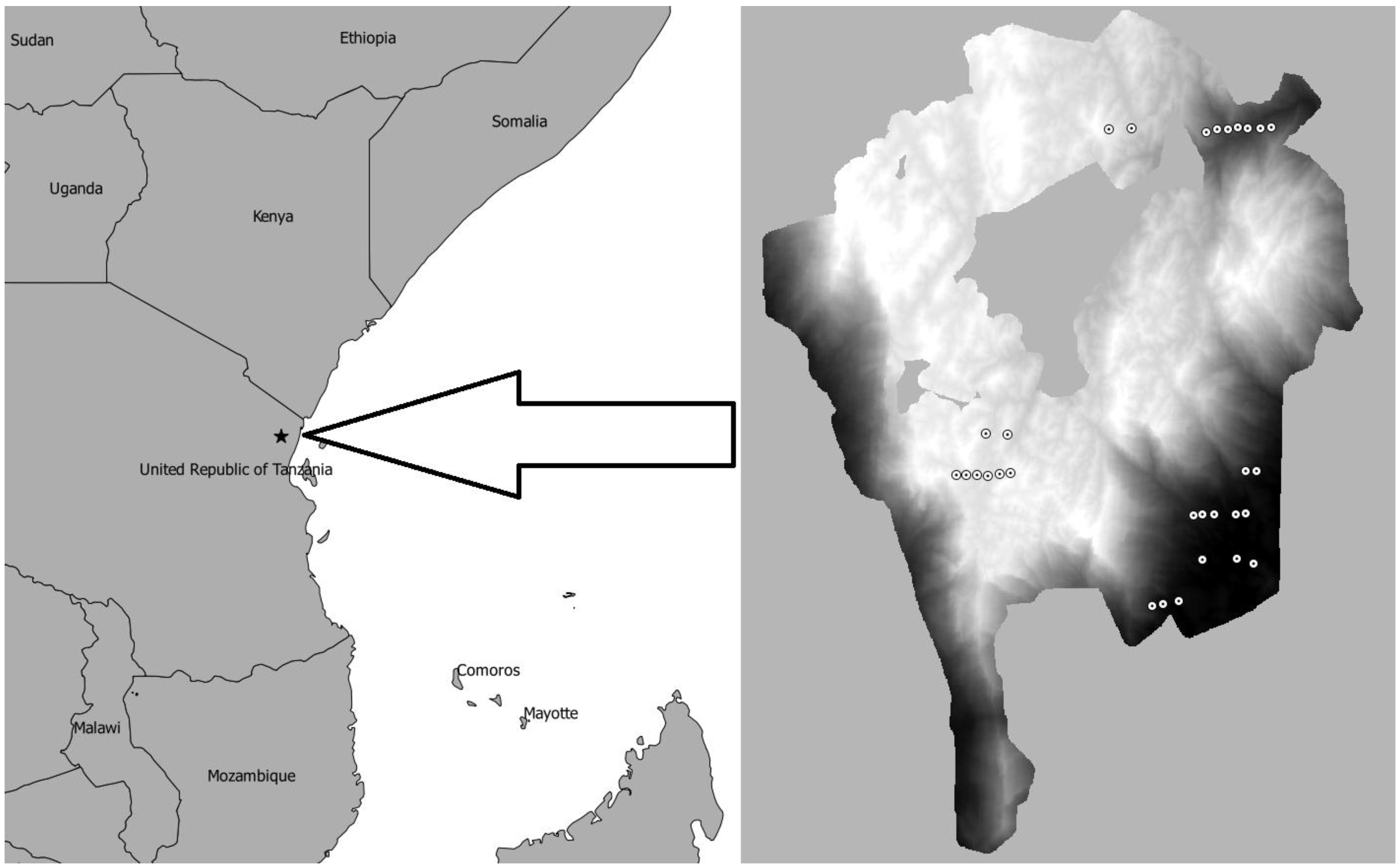
2.1. Study Area

The present study was conducted in the Amani Nature Reserve (ANR) (5°08’S, 38°37’E, 200–1200 m above sea level). The study area covers around 88 km² of tropical submontane rainforest and is located in north-eastern Tanzania and is part of the East Usambara Mountains. The area receives around 2000 mm rainfall per year, and most of the rain falls in the two wet seasons, April–May and October–November. Daily mean temperatures vary from about 16–25 °C. Before the establishment of the ANR in 1997, the area was comprised of six forest reserves and about half of the area was classified as logged or covered with non-native species [27]. After the logging was stopped in the late 1980s most of the logged area recovered and is now secondary forest. Due to inaccessibility the other half of the area had a limited human impact and is considered primary forest.

2.2. Field Data

In the present study we utilized field data (Figure 1) from a sample survey consisting of 30 circular plots collected during November 2011 in pre-determined locations. The plot locations were chosen to capture the variation in biomass by distributing them in different altitudinal zones [16]. To evaluate the representativeness of the 30 circular plots Mauya et al. [16] compared the properties of the sample to a second sample of 153 systematically distributed plots covering the study area. Based on this evaluation Mauya et al. [16] concluded that, although being sampled in an opportunistic manner, the distribution in different altitudinal zones resulted in a sample which closely resembled properties of the systematic sample. The elevation of the 30 circular plots ranged from 223 to 1018 m above sea level with a mean of 552 m.

Figure 1. Left: Study area (marked by star). Right: Field plot locations (marked by dots) inside the Amani Nature Reserve.

Figure 1. Left: Study area (marked by star). Right: Field plot locations (marked by dots) inside the Amani Nature Reserve.

The centre coordinates of the plots were established by means of differential global positioning system (GPS) and global navigation satellite system (GLONASS) using survey-grade receivers. All trees with diameter at breast height (DBH) ≥5 cm were callipered, marked, and species identified. The horizontal distance from the plot centre to the front of each tree was measured using a Vertex IV hypsometer [28]. Because the distance was measured to the front of the trees, half of the tree DBH was added during data processing to get the total horizontal distance to the trees from the plot centre. The heights of three trees per plot (the largest, medium, and smallest tree in terms of DBH) were measured using the hypsometer.

Concentric circular plots of 700, 900, …, 1900 m² were constructed for each of the 30 field plots centred on the positions determined in field. The plot size of 700 m² was chosen because it corresponds to the plot size used in the recently established national forest inventory of Tanzania [29]. The maximum plot size on each location was determined by the reach of the hypsometer, and under the most challenging conditions, distance measurement started to fail at 25 m. Thus, the maximum plot size used in the current study was 1900 m².

Based on the distance from the plot centre to the centre of the stem, each tree was allocated to their respective concentric plot. Biomass of each tree was computed using an allometric model [30] and a diameter to height model developed from the diameters and the corresponding tree heights, see Mauya et al. [16] for further details. The biomass of each tree was then summed at plot level and aggregated biomass was scaled to per-hectare values (Table 1). Although this biomass is referred to as “observed biomass”, the computed values are subject to errors related to the applied allometric model, and the subsampling and measurement of tree DBH and height.

Table 1. Mean biomass and standard deviation (SD) of the 30 field plots with plot sizes of 700, 900, …, 1900 m².

Plot Size(m2)	Mean Biomass(Mg∙ha−1)	SD(Mg∙ha−1)
700	371.8	221.5
900	366.1	216.3
1100	365.6	203.0
1300	361.0	190.5
1500	354.2	180.4
1700	355.0	170.2
1900	351.1	159.6

Table 1. Mean biomass and standard deviation (SD) of the 30 field plots with plot sizes of 700, 900, …, 1900 m².

Plot Size(m2)	Mean Biomass(Mg∙ha−1)	SD(Mg∙ha−1)
700	371.8	221.5
900	366.1	216.3
1100	365.6	203.0
1300	361.0	190.5
1500	354.2	180.4
1700	355.0	170.2
1900	351.1	159.6

2.3. ALS Data

Collection of ALS data with wall-to-wall coverage was carried out from 19 January to 18 February 2012 using a Leica ALS70 sensor mounted on a fixed wing aircraft. The acquisition parameters are summarized in Table 2. Post flight processing of the ALS data was performed by the contractor (Terratec AS, Norway) using TerraScan software [31]. A terrain model was created by classifying ALS echoes as ground echoes using a progressive triangulated irregular network (TIN) densification algorithm [32]. The TIN model was used to calculate the elevation above the ground for all echoes. From the TIN model a raster-based digital terrain model (DTM) with a 10 m × 10 m cell size was created for the entire study area.

Table 2. ALS acquisition parameters.

Parameters	Value
Flight speed (m∙s−1)	70
Flying altitude (m a.g.l.)	800
Scanner frequency (kHz)	339
Footprint size (cm)	22
Beam divergence (mrad)	0.28
Half scan angle (deg.)	16

Table 2. ALS acquisition parameters.

Parameters	Value
Flight speed (m∙s−1)	70
Flying altitude (m a.g.l.)	800
Scanner frequency (kHz)	339
Footprint size (cm)	22
Beam divergence (mrad)	0.28
Half scan angle (deg.)	16

2.4. InSAR Data

InSAR data were acquired by the Tandem-X satellite mission on 6th August 2011. The Tandem-X satellite mission consists of two X-band SAR satellites operating in a pair and provides interferometric images in a single-pass mode. The acquisition had an incidence angle of 46°, was operated in stripmap mode, and the polarization was horizontal transmit and horizontal receive. The normal baseline was 210 m, which corresponded to a 2π height of ambiguity of 38 m. The original spatial resolution of the InSAR data was slightly less than 3 m.

2.5. ALS-Derived Explanatory Variables

ALS echoes were extracted for the concentric circular plots of 700, 900, …, 1900 m² for each of the 30 locations. From a maximum of five echoes registered per ALS pulse, echoes were categorized as “single”, “first of many”, and “last of many”. “Single” and “first of many” were merged into one dataset and denoted as “first” while “single” and “last of many” were merged into another dataset and denoted as “last”. From the ALS echoes in each of the two categories (“first”, “last”), variables describing the height and density of the vegetation were derived. Canopy height variables included percentiles at 10% intervals (H10, H20, …, H90) derived from the laser echoes above a threshold of 2 m above ground. Canopy density variables were computed by first dividing the range between a 95% percentile height and the 2 m threshold into 10 vertical layers of equal height. Further, the proportion of echoes above each layer to the total number of echoes were computed resulting in 10 canopy density variables (D0, D1, …, D9). The variables were computed separately for each echo category (“first”, “last”) and a subscript L or F was used as notation.

The variables were used to construct linear least-square models (Section 2.9) for each of the concentric plot sizes. In order to get comparable results between models from different plot sizes we chose to use the same ALS variables in all models. Studies have shown that a model consisting of one canopy height variable and one canopy density variable is often sufficient for modelling forest biomass [33,34]. In a previous study using the same field and ALS data, Mauya et al. [16] found that the 60th percentile height from the “first” echo category (H60.F) and the proportion of echoes above the second of the 10 vertical layers to the total number of echoes from the “last” echo category (D1.L) were the most frequently selected variables in modelling biomass using plot sizes from 700 to 1900 m². We therefore a priori selected H60.F and D1.L for construction of biomass models.

2.6. InSAR-Derived Explanatory Variable

The Sarscape module of the ENVI 5.0 software was used to process Tandem-X image pairs resulting in a digital surface model (DSM). An interferogram was generated from each image pair, and this was further processed into a differential interferogram by using the ALS DTM as input. Phase noise was removed from the interferogram with a Goldstein filter. Phase offset and phase ramp errors were also removed using 30 ground control points, placed in non-vegetated locations, spread over the study area. Phase unwrapping was carried out using the minimum cost flow method, and the DSM was geocoded to a ground resolution of 10 m × 10 m. Following the construction of the DSM, the DTM derived from the ALS TIN was subtracted from the DSM, resulting in obtained InSAR heights, i.e., heights of the centre of the radar echo above ground. Mean InSAR height was then derived for each field plot by weighting the height of each 10 m × 10 m cell of the normalized InSAR DSM by the area of the cells intersecting the area of the field plot. This mean InSAR height was derived for each concentric field plot area.

2.7. DTM-Derived Explanatory Variable

In a study of forest biomass in two mountain locations in Tanzania, including ANR, Marshall et al. [35] found TE to be positively related to biomass. Therefore, to compare variance estimates obtained using ALS and InSAR, a simple model with TE as the explanatory variable were constructed for each plot size. The DTM derived from the ALS TIN was used to calculate the mean TE for each concentric plot size, 700, 900, …, 1900 m², by weighting the value of each 10 m × 10 m cell of the DTM by the cell area intersected by the plot. The mean TE was subsequently used as an auxiliary variable.

2.8. Tessellating the Study Area and the Remotely Sensed Data

The study area was tessellated into regular grids with hexagonal tiles of 700, 900, …, 1900 m² corresponding to the different plot sizes. To avoid splitting the tiles along the boundary of the study area only tiles with the centroid falling inside of the study area were retained. Remotely sensed variables from ALS and InSAR, along with the TE information were calculated for all hexagonal tiles in the study area.

2.9. Model Construction

For each plot size, separate linear least-square models were constructed with the biomass estimated on the ground plots as response variable and the corresponding remotely sensed variables, from either ALS or InSAR, as explanatory variables. Similarly, simple models were constructed using the TE as explanatory variable. This resulted in a model for each of the three sources of auxiliary data: (1) ALS; (2) InSAR; and (3) TE for each plot size. The general model forms are shown in Table 3. To improve the linear relationship between the explanatory variables and the response, a natural-log transformation of both response and explanatory variable was performed for all models. Such log-log models have been found to be suitable for estimating forest properties using remotely sensed data [33,36,37,38]. This transformation will introduce a bias by back-transformation to arithmetic scale, and a ratio of the mean observed biomass to the mean of the back-transformed estimated biomass proposed by Snowdon [39] was therefore used as a correction factor for the model predictions.

Table 3. General model forms of models using TE, ALS, and InSAR data.

Model	Model Form a
TE	ln(biomass) = ln(terrain elevation)
ALS	ln(biomass) = ln(H60.F) + ln(D1.L)
InSAR	ln(biomass) = ln(InSAR height)

^a Variables explained in Section 2.5, Section 2.6 and Section 2.7.

Table 3. General model forms of models using TE, ALS, and InSAR data.

Model	Model Form a
TE	ln(biomass) = ln(terrain elevation)
ALS	ln(biomass) = ln(H60.F) + ln(D1.L)
InSAR	ln(biomass) = ln(InSAR height)

^a Variables explained in Section 2.5, Section 2.6 and Section 2.7.

Unlike design-based estimators, which often are unbiased or nearly unbiased, the unbiasedness of model-based estimators depends on the model being correctly specified. It was therefore paramount to assess how well the model fit the field plot observations. Assessment of the fit of the models followed the approach used by McRoberts et al. [40]. Scatterplots of observed vs. predicted biomass were produced for each plot size. Correctly specified models should result in points falling closely along a 1:1 line with intercept 0 and slope 1. Further, pairs of observations and predictions were ordered with respect to the predicted values and grouped into three classes of 10 pairs. The mean of the observed versus predicted biomass was plotted for each group. A correctly specified model should again result in points falling along a 1:1 line.

2.10. Model-Based Inference

Model-based inference does not, as opposed to design-based inference, rely on a probabilistic sample that represents the population. Instead, as stated above, the inference relies on the model itself as a valid model of a superpopulation. Following the notation in Ståhl et al. [41] an element of the superpopulation was expressed as

$${\text{y}}_{\mathrm{i}}=\text{g}\left({\text{x}}_{\mathrm{i}},\text{ α},{\text{ε}}_{\mathrm{i}}\right)$$

(1)

where $\text{y}$ is a vector of the observed plot biomass on plot $\text{i}$, $\text{x}$ is a vector of variables derived from the auxiliary data, $\text{α}$ is a vector of model parameters and $\text{ε}$ is a vector of errors, and $\text{g}$ is a function describing the superpopulation. It is assumed that the errors are independent, normally distributed, with a constant variance, and without spatial auto-correlation. The parameters $\text{α}$ were estimated with $\widehat{\text{α}}$ using least square regression, and used to estimate the population mean by

$$\widehat{\text{μ}}=\frac{1}{\text{N}}{{\displaystyle \sum }}_{\text{i}=1}^{\text{N}}\text{g}\left({\text{x}}_{\mathrm{i}},\widehat{\text{α}}\right)$$

(2)

where i indexes the population elements and N is the number of elements, i.e., i=1, 2, …, N. Assuming that the estimated $\widehat{\text{α}}$ is accurate, the $\text{g}$ function was linearized in the neighbourhood of the true function using first order Taylor series expansion. Details of the derivation of the function is given in Appendix A of Ståhl et al. [41]. The variance of the population mean was then estimated by

$$\widehat{\text{var}}\left(\widehat{\text{μ}}\right)={{\displaystyle \sum }}_{\text{j}=1}^{\text{p}}{{\displaystyle \sum }}_{\text{k}=1}^{\text{p}}\widehat{\text{Cov}}\left({\widehat{\text{α}}}_{\text{j}},{\widehat{\text{α}}}_{\text{k}}\right){\widehat{\overline{\text{g}}}}_{\text{j}}^{\prime }{\widehat{\overline{\text{g}}}}_{\text{k}}^{\prime }$$

(3)

where ${\widehat{\overline{\text{g}}}}_{\text{j}}^{\prime }$ and ${\widehat{\overline{\text{g}}}}_{\text{k}}^{\prime }$ are the estimated mean values of the first order derivatives of the $\text{g}$ function for parameters j and k (j = 1, 2, …, k, …,), respectively (cf. [41]). Standard errors (SE) of the mean estimates, i.e., the square root of the variance estimate $\left(\sqrt{\widehat{\text{var}}\left(\widehat{\text{μ}}\right)}\right)$, were reported along with SE relative to the mean estimates.

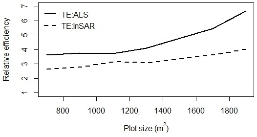
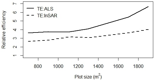
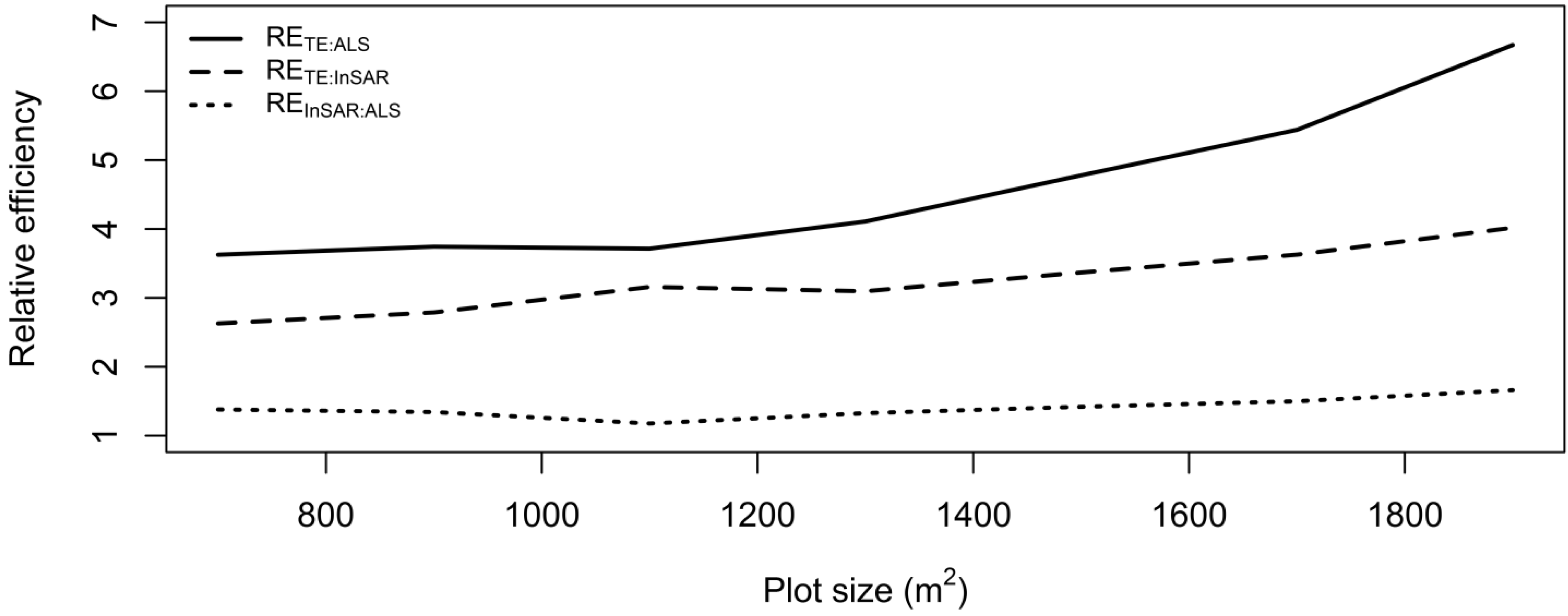
2.11. Relative Efficiency

To assess the gain in precision of using remotely sensed data to enhance the estimates, relative efficiency was calculated for both ALS (RE_TE:ALS) and InSAR (RE_TE:InSAR). The relative efficiencies were calculated as ratios of the estimated variance for the mean biomass estimate ($\widehat{\text{μ}}$) for each plot size using the TE models divided by the variance estimates for each plot size using the ALS models:

$${\text{RE}}_{\text{TE}:{\text{ALS}}_{\text{s}}}=\widehat{\text{var}}{\left({\widehat{\text{μ}}}_{\text{TE}}\right)}_{\text{s}}/\widehat{\text{var}}{\left({\widehat{\text{μ}}}_{\text{ALS}}\right)}_{\text{s}}$$

(4)

where s is an indicator of the plot sizes 700, 900, …, 1900 m². Similarly, relative efficiency for InSAR was computed as:

$${\text{RE}}_{\text{TE}:{\text{InSAR}}_{\text{s}}}=\widehat{\text{var}}{\left({\widehat{\text{μ}}}_{\text{TE}}\right)}_{\text{s}}/\widehat{\text{var}}{\left({\widehat{\text{μ}}}_{\text{InSAR}}\right)}_{\text{s}}$$

(5)

Efficiency of ALS was also calculated relative to InSAR (RE_InSAR:ALS) in the same way by dividing the variance estimates for each plot size using the InSAR models by the variance estimates for each plot size using the ALS models:

$${\text{RE}}_{\text{InSAR}:{\text{ALS}}_{\text{s}}}=\widehat{\text{var}}{\left({\widehat{\text{μ}}}_{\text{InSAR}}\right)}_{\text{s}}/\widehat{\text{var}}{\left({\widehat{\text{μ}}}_{\text{ALS}}\right)}_{\text{s}}$$

(6)

Together with information about inventory costs and the costs of the auxiliary data, the relative efficiency can be used to compare costs of attaining a certain level of precision of the estimation. In a design-based framework, applying simple random sampling (SRS), the relative efficiency can be used directly to calculate the additional number of field observations needed to compensate for the contribution of the remotely sensed data, which is a fundamental quantity in cost comparisons. This is because the SE of the mean estimate under SRS is proportional to the square root of the sample size minus the number of explanatory variables minus one ([42] p. 181). In practice, a relative efficiency of two would mean that the gain of the remotely sensed data could be compensated by twice as many field plots, assuming that the sample variance remains constant. In the model-based framework we also assume that the SE of the mean estimate is reduced with increased number of observations. However, we are not able to derive the number of observations needed to reach the same SE for the different models by analytical means. Instead we applied a basic Pólya-urn resampling scheme described in Köhl et al. ([22], pp. 195–196) to simulate the variance of the TE models. The Pólya-urn resampling scheme generates a design-consistent posterior predictive distribution of the property in interest, given that the sample is reasonably large and representative of the population ([43], pp. 44–46). We consider our field sample of u=30 observations as representative of the population, and the Pólya-urn resampling generated posterior predictive distributions of biomass for U = 60, 120, and 180 observations based on the sample. From a virtual urn, containing the 30 observations, one observation was randomly drawn, duplicated, and returned to the urn together with the duplicate. The urn thus contained u + 1 = 31 observations. The selection scheme was repeated until the desired number U of observations in the urn was reached. The simulations were repeated 200 times and the mean variance of observed biomass reported.

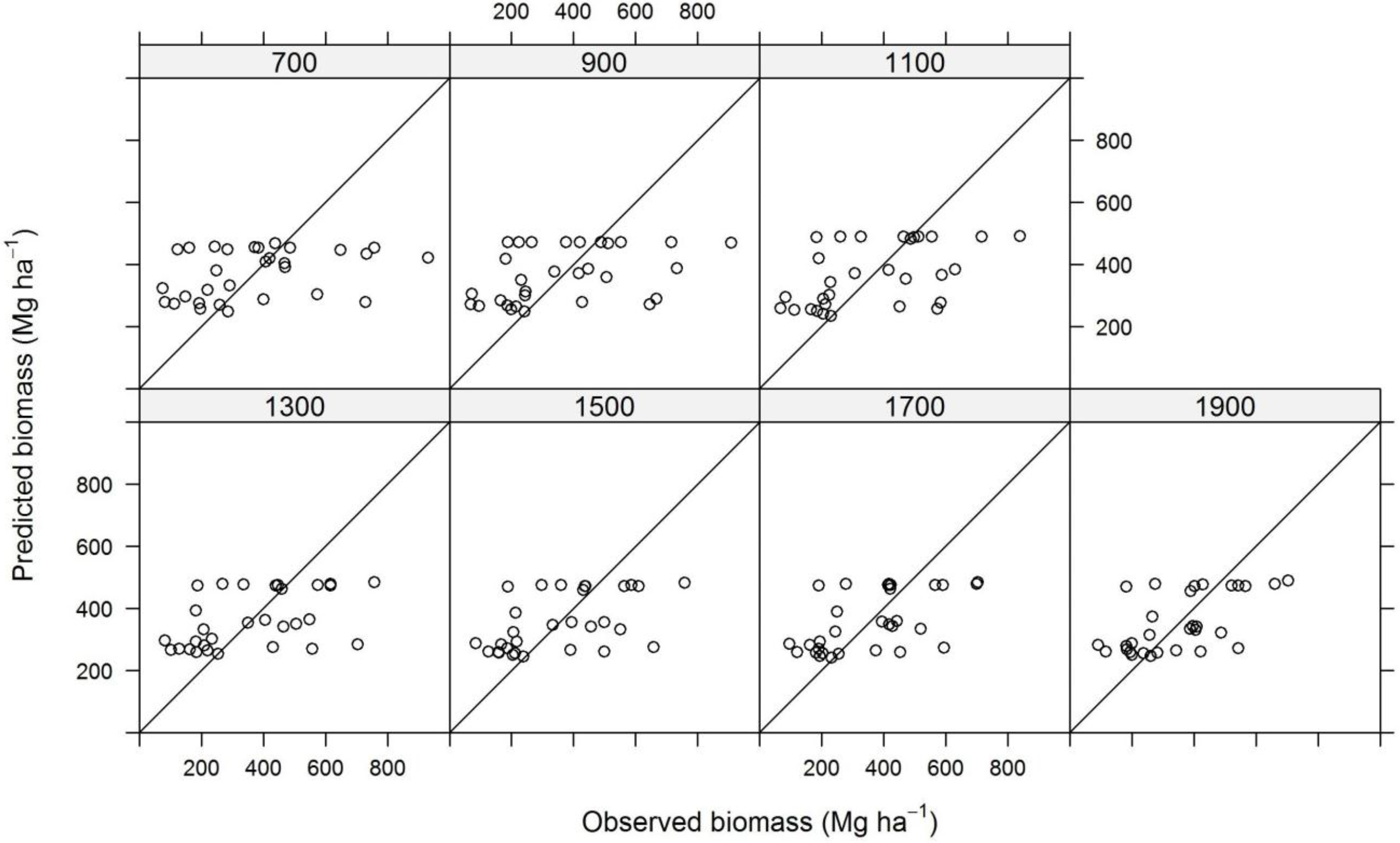
3. Results and Discussion

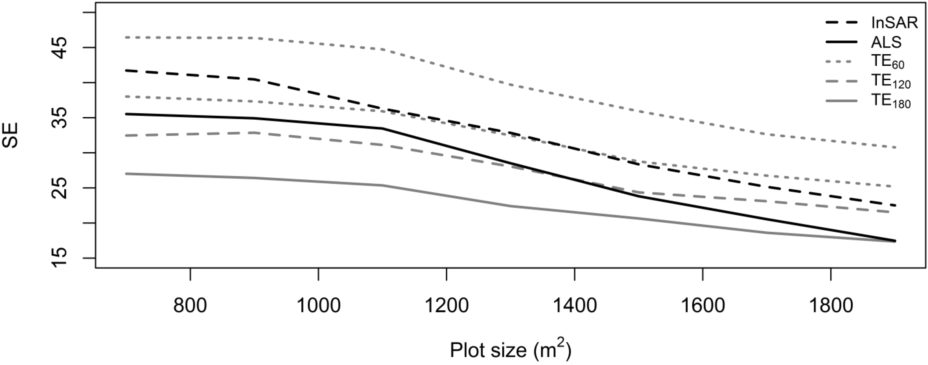
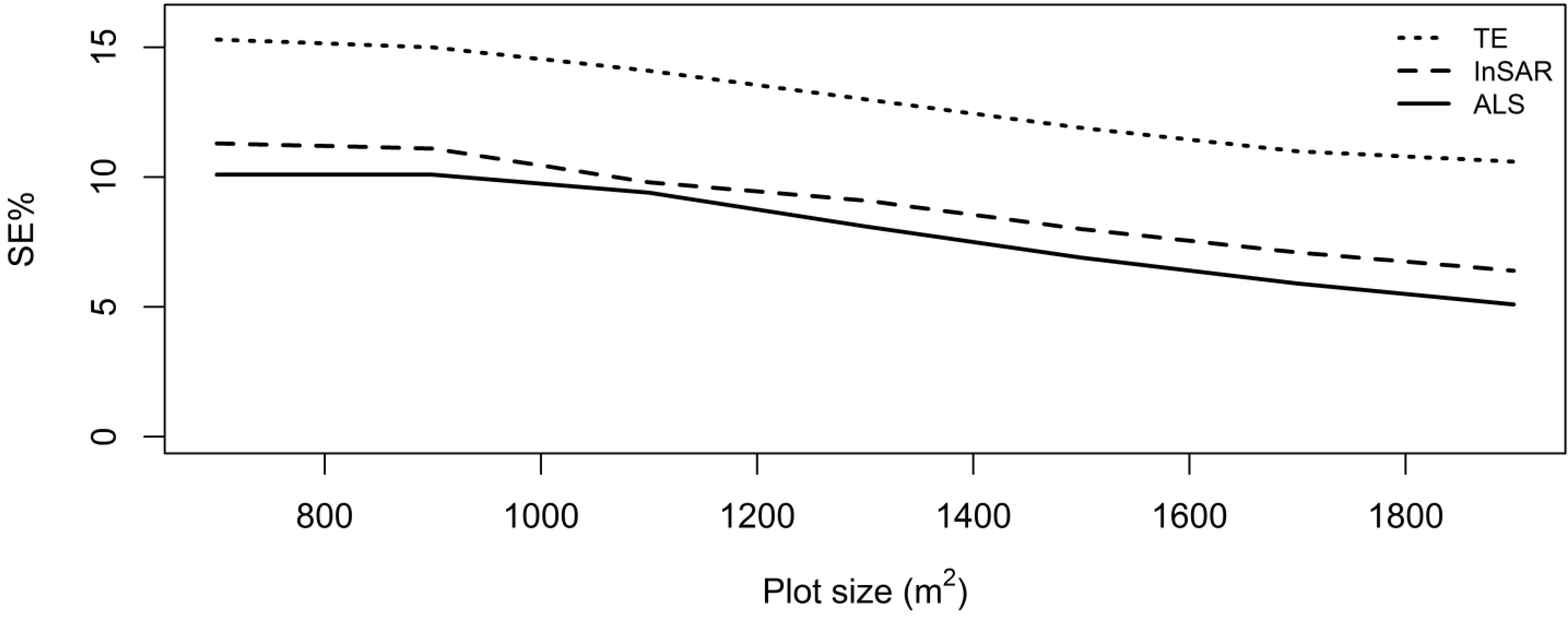
Use of remotely sensed data to support field-based sample surveys will be part of any REDD+ MRV system. Better information on how the relative efficiency of using remotely sensed data is affected by plot size would benefit future MRV designs. The findings in the present study demonstrate the impact of the size of the field plots on the precision of biomass estimates using two types of three-dimensional remotely sensed data.

Separate log-log models were constructed for each plot size of 700, 900, …, 1900 m² using auxiliary data from (1) ALS; (2) InSAR; and (3) TE. TE models showed a positive correlation between biomass and elevation, and the explanatory variable was increasingly significant from p = 0.044 at 700 m² to p = 0.002 at 1900 m². Biomass was also positively correlated to the two explanatory variables in the ALS models describing the height and density of the forest canopy (H60.F, D1.L) and the variable in the InSAR models, the above ground height of the InSAR radar echo. All variables were significant at a 95% level except one of the ALS variables (D1.L) at plot sizes of 1100–1700 m².

Inspection of the scatterplots of observed versus predicted biomass (Figure 2, Figure 3 and Figure 4) showed that the models had a lack of fit resulting in over-prediction of biomass in areas of low biomass and under-prediction in areas of high biomass. Similar lack of fit has been reported in studies from areas with high biomass values (e.g., [44,45]). The plots of the grouped means of observations versus predictions (Figure 5, Figure 6, and Figure 7), however, showed small differences.

Figure 2. Observed versus predicted biomass values using ALS for plot sizes of 700, 900, …, 1900 m².

Figure 2. Observed versus predicted biomass values using ALS for plot sizes of 700, 900, …, 1900 m².

Figure 3. Observed versus predicted biomass values using InSAR for plot sizes of 700, 900, …, 1900 m².

Figure 3. Observed versus predicted biomass values using InSAR for plot sizes of 700, 900, …, 1900 m².

Figure 4. Observed versus predicted biomass values using TE for plot sizes of 700, 900, …, 1900 m².

Figure 4. Observed versus predicted biomass values using TE for plot sizes of 700, 900, …, 1900 m².

Figure 5. Grouped means of observed versus predicted biomass values using ALS for plot sizes of 700, 900, …, 1900 m².

Figure 5. Grouped means of observed versus predicted biomass values using ALS for plot sizes of 700, 900, …, 1900 m².

Figure 6. Grouped means of observed versus predicted biomass values using InSAR for plot sizes of 700, 900, …, 1900 m².

Figure 6. Grouped means of observed versus predicted biomass values using InSAR for plot sizes of 700, 900, …, 1900 m².

Figure 7. Grouped means of observed versus predicted biomass values using TE for plot sizes of 700, 900, …, 1900 m².

Figure 7. Grouped means of observed versus predicted biomass values using TE for plot sizes of 700, 900, …, 1900 m².

As pointed out in Section 2.2, the observed biomass is subject to uncertainty not accounted for in the present study, related to the allometric models and field measurements of DBH and tree height. Thus, errors related to the biomass observations are not accounted for. Overlooking these errors lead to overoptimistic precision of the variance estimates. In a study conducted in a tropical forest in Ghana, in which the forest conditions and the plot size of 1600 m² resembled the conditions in the present study, Chen et al. [46] found that the impact of allometric error contributed about 11% to the total relative prediction error.

Mean biomass estimates of the ANR from both ALS and InSAR were lower than the mean estimate from the model with TE (Table 4). The differences were however not statistically significant at the 5% level.

Table 4. Estimated mean biomass ($\widehat{\text{μ}}$) in Mg∙ha⁻¹ and standard error of the estimate (SE) in Mg∙ha⁻¹ and in % of the mean estimate for three different sources of auxiliary data (terrain elevation (TE), ALS, and InSAR).

Plot Size	N	TE			ALS			InSAR
		$\widehat{\text{μ}}$ (Mg∙ha−1)	SE (Mg∙ha−1)	SE (%)	$\widehat{\text{μ}}$ (Mg∙ha−1)	SE (Mg∙ha−1)	SE (%)	$\widehat{\text{μ}}$ (Mg∙ha−1)	SE (Mg∙ha−1)	SE (%)
700	126,772	442.2	67.6	15.3	352.9	35.5	10.1	368.0	41.7	11.3
900	98,635	449.1	67.6	15.0	346.1	34.9	10.1	365.7	40.5	11.1
1100	80,667	458.6	64.5	14.1	356.3	33.5	9.4	369.1	36.3	9.8
1300	68,279	443.6	57.8	13.0	350.5	28.5	8.1	361.0	32.8	9.1
1500	59,154	435.7	52.1	11.9	345.5	23.8	6.9	354.2	28.4	8.0
1700	52,214	435.0	47.9	11.0	346.4	20.5	5.9	354.2	25.2	7.1
1900	46,727	427.2	45.1	10.6	341.4	17.5	5.1	350.3	22.5	6.4

Table 4. Estimated mean biomass ($\widehat{\text{μ}}$) in Mg∙ha⁻¹ and standard error of the estimate (SE) in Mg∙ha⁻¹ and in % of the mean estimate for three different sources of auxiliary data (terrain elevation (TE), ALS, and InSAR).

Plot Size	N	TE			ALS			InSAR
		$\widehat{\text{μ}}$ (Mg∙ha−1)	SE (Mg∙ha−1)	SE (%)	$\widehat{\text{μ}}$ (Mg∙ha−1)	SE (Mg∙ha−1)	SE (%)	$\widehat{\text{μ}}$ (Mg∙ha−1)	SE (Mg∙ha−1)	SE (%)
700	126,772	442.2	67.6	15.3	352.9	35.5	10.1	368.0	41.7	11.3
900	98,635	449.1	67.6	15.0	346.1	34.9	10.1	365.7	40.5	11.1
1100	80,667	458.6	64.5	14.1	356.3	33.5	9.4	369.1	36.3	9.8
1300	68,279	443.6	57.8	13.0	350.5	28.5	8.1	361.0	32.8	9.1
1500	59,154	435.7	52.1	11.9	345.5	23.8	6.9	354.2	28.4	8.0
1700	52,214	435.0	47.9	11.0	346.4	20.5	5.9	354.2	25.2	7.1
1900	46,727	427.2	45.1	10.6	341.4	17.5	5.1	350.3	22.5	6.4

Increasing the plot size from 700 to 1900 m² reduced the SE of the mean estimates from 15.3% to 10.6% using TE, from 10.1% to 5.1% using ALS, and from 11.3%–6.4% using InSAR (Figure 8). Both ALS and InSAR performed well compared to TE in terms of SE. ALS and InSAR estimates had an SE of about 5 and 4 percentage points lower than TE, respectively. Further, InSAR performed well compared to the ALS with only 0.4–1.3 percentage points higher SE depending on plot size. The differences in SE translated into relative efficiencies of 3.6–6.7 using ALS and 2.6–4.0 using InSAR, compared to TE (Figure 9). The relative efficiency of the ALS data also increased with increased plot size relative also to the InSAR data (Figure 9). At a plot size of 1900 m² the ALS was 6.7 times as efficient as using TE and 1.7 times as efficient as InSAR. The fact that the relative efficiency of ALS and InSAR increased with increased plot size may partly be due to reduced relative influence of boundary effects and co-registration errors. The slight increase in relative efficiency of ALS compared to InSAR may also indicate that the relative influence of boundary effects and co-registration errors is stronger for ALS than for InSAR. The relative efficiency of ALS compared to InSAR is modest compared to studies in Norway that have found the relative efficiency of ALS to be about twice to that of InSAR [34,47].

Figure 8. Relative standard error of biomass estimates (SE%) using models with auxiliary data of terrain elevation (TE) derived from a digital terrain model (dotted line), InSAR (dashed line), and ALS (solid line).

Figure 8. Relative standard error of biomass estimates (SE%) using models with auxiliary data of terrain elevation (TE) derived from a digital terrain model (dotted line), InSAR (dashed line), and ALS (solid line).

Figure 9. Relative efficiency of using InSAR (RE_TE:InSAR, dashed line) and ALS (RE_TE:ALS, solid line) relative to TE for biomass estimation, and ALS relative to InSAR (RE_InSAR:ALS, dotted line).

Figure 9. Relative efficiency of using InSAR (RE_TE:InSAR, dashed line) and ALS (RE_TE:ALS, solid line) relative to TE for biomass estimation, and ALS relative to InSAR (RE_InSAR:ALS, dotted line).

As stated by Gregoire et al. [48], information about the approach to statistical inference, design- or model-based, is essential in assessing the estimated variance. Taking the design-based approach to variance estimation d'Oliveira et al. [49], reported a relative efficiency of 3.4 in a study utilising 50 plots of $~$0.25 ha in the Brazilian Amazon. We can similarly compute the relative efficiency from the variance estimates reported by Hansen et al. [10]. For a plot size of $~$0.1 ha the relative efficiency was 2.1. The latter study discusses large negative boundary-effects in the ALS-derived variables, which would contribute to a low relative efficiency.

The DTM used directly to derive the TE variable in the TE-models, and to derive the InSAR elevation above the terrain, was derived from the ALS data. DTMs constructed from ALS data have generally high accuracy [50]. In the absence of an ALS-derived DTM, a DTM derived from other sources would have influenced the results. A DTM derived from sources like P-band SAR (e.g., [51]) or the topographic map series of Tanzania, would most likely have resulted in substantially increased SE of the InSAR and TE estimates. In a study using InSAR height to estimate forest biomass in Norway Næsset et al. [34] it was found that relative RMSE was approximately seven percentage points higher using a DTM from topographic maps with a contour interval of 20 m, compared to using an ALS-derived DTM. P-band SAR, used with good results in Neeff et al. [51], is currently only available from airborne platforms, and was not collected in ANR.

The analysis in the present study showed that use of remotely sensed data from ALS and InSAR was able to increase the precision of the estimates. However, ALS data are expensive compared to the marginal cost of establishing additional inventory plots (100–150 USD per plot [52]). The effect of increased number of field plots on the sampling error of the TE models was simulated using a Pólya-urn resampling scheme. To reach similar levels of sampling error as for the ALS models, the number of field plots would have to be increased by a factor of 3.5–6 depending on plot size (Figure 10).

Figure 10. Standard error of biomass estimates (SE) using models with auxiliary data of InSAR (dashed line), ALS (solid line), and TE. TE model SE is derived from 60 (dotted grey line), 120 (dashed grey line), and 180 (solid grey line) simulated observations.

Figure 10. Standard error of biomass estimates (SE) using models with auxiliary data of InSAR (dashed line), ALS (solid line), and TE. TE model SE is derived from 60 (dotted grey line), 120 (dashed grey line), and 180 (solid grey line) simulated observations.

With the relatively low cost of increasing the intensity of the field inventory (180 plots × a cost of 125 USD = 22,500 USD), the increased precision of using ALS is not solely enough to defend the investment of about 100,000 USD for the ALS mission. However, ALS does provide a good quality DTM which can be used for future surveys supported by other sources of remotely sensed data requiring such a DTM. The cost of ALS is largely governed by the flight time. By flying higher, covering a larger area with a single flight strip, the cost of acquiring ALS can be reduced. Findings from studies of reduced pulse density either by means of simulations (e.g., [53]), or acquisitions from different altitudes (e.g., [54]), have shown that satisfactory results can be attained at lower pulse densities. A simulation study conducted in ANR [55], confirmed that explanatory variables derived from low pulse density is reliable down to about 0.5 pulses·m⁻², even in dense tropical forests. Although the study [55] does not present results on RMSEs of a subsequent biomass model, the standard deviation of the digital terrain model was stabile down to about 0.5 pulses·m⁻². Because variance in the terrain model is carried forward into the explanatory variables in a biomass model, the RMSEs obtained with lower pulse densities would also be stabile down to about 0.5 pulses·m⁻².

4. Conclusions

The results from the present study demonstrated, in accordance with earlier studies, that auxiliary remotely sensed information could be utilized to increase the precision of biomass estimates in tropical forests. Further, the results showed that the relative efficiency of using remotely sensed data from both ALS and InSAR sensors increased with increased field plot size. Thus, biomass estimation assisted by remotely sensed data from ALS and InSAR will profit relatively more in terms of increased precision by increasing plot size than estimation without ALS and InSAR data. The relative efficiency of both ALS and InSAR increased continuously with increased plot sizes. To compensate for a lack of ALS data the pure field-based inventory would have to contain 3.5–6.0 times as many observations for plot sizes of 700–1900 m² to achieve the same precision as an inventory supported by ALS data. Many tropical countries are about to establish their first nation-wide forest sample surveys and plot size is a survey design parameter that must be considered in light of future use of remotely sensed data to enhance estimation. Thus, it is important to quantify the influence of plot size on estimation efficiency of biomass in various forest types found in tropical countries to inform design and investment decisions in future surveys.

References

1. UNFCCC. Report of the Conference of the Parties on its Sixteenth Session, held in Cancun from 29 November to 10 December 2010. Addendum. Part two: Action taken by the Conference of the Parties at its Sixteenth Session; United Nations Office: Geneva, Switzerland, 2011; p. 31. [Google Scholar]
2. UNFCCC. Report of the Conference of the Parties on its Fifteenth Session, held in Copenhagen from 7 to 19 December 2009. Addendum. Part Two: Action taken by the Conference of the Parties at its Fifteenth Session; United Nations Office: Geneva, Switzerland, 2010; p. 43. [Google Scholar]
3. FAO. Forest resources of the world. In Unasylva; 1948; Available online: http://www.fao.org/docrep/x5345e/x5345e00.htm (accessed on 16 January 2015).
4. Boyd, D.S.; Danson, F.M. Satellite remote sensing of forest resources: Three decades of research development. Progr. Phys. Geogr. 2005, 29, 1–26. [Google Scholar] [CrossRef]
5. Bohlin, J.; Wallerman, J.; Fransson, J.E.S. Forest variable estimation using photogrammetric matching of digital aerial images in combination with a high-resolution DEM. Scand. J. Forest Res. 2012, 27, 692–699. [Google Scholar] [CrossRef]
6. Persson, H.; Wallerman, J.; Olsson, H.; Fransson, J.E.S. Estimating forest biomass and height using optical stereo satellite data and a DTM from laser scanning data. Can. J. Remote Sens. 2013, 39, 251–262. [Google Scholar] [CrossRef]
7. Gobakken, T.; Bollandsås, O.M.; Næsset, E. Comparing biophysical forest characteristics estimated from photogrammetric matching of aerial images and airborne laser scanning data. Scand. J. Forest Res. 2014, 30, 1–14. [Google Scholar] [CrossRef]
8. Næsset, E. Determination of mean tree height of forest stands by digital photogrammetry. Scand. J. Forest Res. 2002, 17, 446–459. [Google Scholar] [CrossRef]
9. Zolkos, S.G.; Goetz, S.J.; Dubayah, R. A meta-analysis of terrestrial aboveground biomass estimation using lidar remote sensing. Remote Sens. Environ. 2013, 128, 289–298. [Google Scholar] [CrossRef]
10. Hansen, E.; Gobakken, T.; Bollandsås, O.; Zahabu, E.; Næsset, E. Modeling aboveground biomass in dense tropical submontane rainforest using airborne laser scanner data. Remote Sens. 2015, 7, 788–807. [Google Scholar] [CrossRef] [Green Version]
11. Fassnacht, F.E.; Hartig, F.; Latifi, H.; Berger, C.; Hernández, J.; Corvalán, P.; Koch, B. Importance of sample size, data type and prediction method for remote sensing-based estimations of aboveground forest biomass. Remote Sens. Environ. 2014, 154, 102–114. [Google Scholar] [CrossRef]
12. Gobakken, T.; Næsset, E. Assessing effects of positioning errors and sample plot size on biophysical stand properties derived from airborne laser scanner data. Can. J. For. Res. 2009, 39, 1036–1052. [Google Scholar] [CrossRef]
13. Mascaro, J.; Detto, M.; Asner, G.P.; Muller-Landau, H.C. Evaluating uncertainty in mapping forest carbon with airborne LiDAR. Remote Sens. Environ. 2011, 115, 3770–3774. [Google Scholar] [CrossRef]
14. Frazer, G.W.; Magnussen, S.; Wulder, M.A.; Niemann, K.O. Simulated impact of sample plot size and co-registration error on the accuracy and uncertainty of LiDAR-derived estimates of forest stand biomass. Remote Sens. Environ. 2011, 115, 636–649. [Google Scholar] [CrossRef]
15. Hernández-Stefanoni, J.; Dupuy, J.; Johnson, K.; Birdsey, R.; Tun-Dzul, F.; Peduzzi, A.; Caamal-Sosa, J.; Sánchez-Santos, G.; López-Merlín, D. Improving species diversity and biomass estimates of tropical dry forests using airborne LiDAR. Remote Sens. 2014, 6, 4741–4763. [Google Scholar] [CrossRef]
16. Mauya, E.; Hansen, E.H.; Gobakken, T.; Bollandsås, O.M.; Malimbwi, R.E.; Næsset, E. Effects of field plot size on prediction accuracy of aboveground biomass in airborne laser scanning-assisted inventories in tropical rain forests of Tanzania. Carbon Balanc. Manage. 2015. submitted. [Google Scholar] [CrossRef] [PubMed] [Green Version]
17. Næsset, E. Determination of mean tree height of forest stands using airborne laser scanner data. ISPRS J. Photogramm. Remote Sens. 1997, 52, 49–56. [Google Scholar] [CrossRef]
18. Næsset, E. Estimating timber volume of forest stands using airborne laser scanner data. Remote Sens. Environ. 1997, 61, 246–253. [Google Scholar] [CrossRef]
19. Næsset, E.; Bollandsås, O.M.; Gobakken, T. Comparing regression methods in estimation of biophysical properties of forest stands from two different inventories using laser scanner data. Remote Sens. Environ. 2005, 94, 541–553. [Google Scholar] [CrossRef]
20. Li, Y.Z.; Andersen, H.E.; McGaughey, R. A comparison of statistical methods for estimating forest biomass from light detection and ranging data. West. J. Appl. For. 2008, 23, 223–231. [Google Scholar]
21. Clark, D.B.; Kellner, J.R. Tropical forest biomass estimation and the fallacy of misplaced concreteness. J. Veg. Sci. 2012, 23, 1191–1196. [Google Scholar] [CrossRef]
22. Köhl, M.; Magnussen, S.; Marchetti, M. Sampling Methods, Remote Sensing and GIS Multiresource Forest Inventory; Springer: Berlin, Germany, 2006; p. 365. [Google Scholar]
23. Gregoire, T.G. Design-based and model-based inference in survey sampling: Appreciating the difference. Can. J. For. Res. 1998, 28, 1429–1447. [Google Scholar] [CrossRef]
24. Payandeh, B. Relative efficiency of two-dimensional systematic sampling. For. Sci. 1970, 16, 271–276. [Google Scholar]
25. Ene, L.T.; Næsset, E.; Gobakken, T.; Gregoire, T.G.; Stahl, G.; Nelson, R. Assessing the accuracy of regional LiDAR-based biomass estimation using a simulation approach. Remote Sens. Environ. 2012, 123, 579–592. [Google Scholar] [CrossRef]
26. Næsset, E. Area-based inventory in Norway—From innovation to an operational reality. In Forestry Applications of Airborne Laser Scanning; Maltamo, M., Næsset, E., Vauhkonen, J., Eds.; Springer: Dordrecht, The Netherlands, 2014; Volume 27, pp. 215–240. [Google Scholar]
27. Hamilton, A.C.; Bensted-Smith, R. Forest Conservation in the East Usambara Mountains, Tanzania; IUCN-The World Conservation Union; Dar es Salaam, Tanzania: Forest Division, Ministry of Lands, Natural Resources, and Tourism, United Republic of Tanzania: Gland, Switzerland/Cambridge, UK, 1989; p. 392. [Google Scholar]
28. Haglöf Sweden. Users Guide Vertex III V1.5 and Transponder T3; Haglöf Sweden AB: Långsele, Sweden, 2007. [Google Scholar]
29. Tomppo, E.; Malimbwi, R.; Katila, M.; Mäkisara, K.; Henttonen, H.M.; Chamuya, N.; Zahabu, E.; Otieno, J. A sampling design for a large area forest inventory: Case Tanzania. Can. J. For. Res. 2014, 44, 931–948. [Google Scholar] [CrossRef]
30. Masota, A.M.; Zahabu, E.; Malimbwi, R.; Bollandsås, O.M.; Eid, T. Tree allometric models for above- and belowground biomass of tropical rainforests in Tanzania. South. For. J. Forest Sci. 2015. submitted. [Google Scholar]
31. Soininen, A. TerraScan User’s Guide; Terrasolid Oy: Jyvaskyla, Finland, 2012. [Google Scholar]
32. Axelsson, P. DEM generation from laser scanner data using adaptive TIN models. Int. Arch. Photogramm. Remote Sens. Spat. Inf. Sci. 2000, 33, 110–117. [Google Scholar]
33. Ioki, K.; Tsuyuki, S.; Hirata, Y.; Phua, M.-H.; Wong, W.V.C.; Ling, Z.-Y.; Saito, H.; Takao, G. Estimating above-ground biomass of tropical rainforest of different degradation levels in Northern Borneo using airborne LiDAR. For. Ecol. Manage. 2014, 328, 335–341. [Google Scholar] [CrossRef]
34. Næsset, E.; Gobakken, T.; Solberg, S.; Gregoire, T.G.; Nelson, R.; Stahl, G.; Weydahl, D. Model-assisted regional forest biomass estimation using LiDAR and InSAR as auxiliary data: A case study from a boreal forest area. Remote Sens. Environ. 2011, 115, 3599–3614. [Google Scholar] [CrossRef]
35. Marshall, A.R.; Willcock, S.; Platts, P.J.; Lovett, J.C.; Balmford, A.; Burgess, N.D.; Latham, J.E.; Munishi, P.K.T.; Salter, R.; Shirima, D.D.; et al. Measuring and modelling above-ground carbon and tree allometry along a tropical elevation gradient. Biol. Conserv. 2012, 154, 20–33. [Google Scholar]
36. Means, J.E.; Acker, S.A.; Harding, D.J.; Blair, J.B.; Lefsky, M.A.; Cohen, W.B.; Harmon, M.E.; McKee, W.A. Use of large-footprint scanning airborne lidar to estimate forest stand characteristics in the Western Cascades of Oregon. Remote Sens. Environ. 1999, 67, 298–308. [Google Scholar] [CrossRef]
37. Lim, K.; Treitz, P.; Baldwin, K.; Morrison, I.; Green, J. LiDAR remote sensing of biophysical properties of tolerant northern hardwood forests. Can. J. Remote Sens. 2003, 29, 658–678. [Google Scholar] [CrossRef]
38. Næsset, E. Predicting forest stand characteristics with airborne scanning laser using a practical two-stage procedure and field data. Remote Sens. Environ. 2002, 80, 88–99. [Google Scholar] [CrossRef]
39. Snowdon, P. A ratio estimator for bias correction in logarithmic regressions. Can. J. For. Res. 1991, 21, 720–724. [Google Scholar] [CrossRef]
40. McRoberts, R.E.; Næsset, E.; Gobakken, T. Inference for LiDAR-assisted estimation of forest growing stock volume. Remote Sens. Environ. 2013, 128, 268–275. [Google Scholar] [CrossRef]
41. Ståhl, G.; Holm, S.; Gregoire, T.G.; Gobakken, T.; Næsset, E.; Nelson, R. Model-based inference for biomass estimation in a LiDAR sample survey in Hedmark County, Norway. Can. J. For. Res. 2011, 41, 96–107. [Google Scholar] [CrossRef]
42. Stoltzenberg, R.M. Multiple regression analysis. In Handbook of Data Analysis; Hardy, M.A., Bryman, A., Eds.; SAGE Publications Ltd: London, UK, 2009; pp. 165–207. [Google Scholar]
43. Ghosh, M.; Meeden, G. Bayesian Methods for Finite Population Sampling; Chapman & Hall: London, UK, 1997. [Google Scholar]
44. Vincent, G.; Sabatier, D.; Blanc, L.; Chave, J.; Weissenbacher, E.; Pélissier, R.; Fonty, E.; Molino, J.F.; Couteron, P. Accuracy of small footprint airborne LiDAR in its predictions of tropical moist forest stand structure. Remote Sens. Environ. 2012, 125, 23–33. [Google Scholar] [CrossRef]
45. Nord-Larsen, T.; Schumacher, J. Estimation of forest resources from a country wide laser scanning survey and national forest inventory data. Remote Sens. Environ. 2012, 119, 148–157. [Google Scholar] [CrossRef]
46. Chen, Q.; Vaglio Laurin, G.; Valentini, R. Uncertainty of remotely sensed aboveground biomass over an African tropical forest: Propagating errors from trees to plots to pixels. Remote Sens. Environ. 2015, 160, 134–143. [Google Scholar] [CrossRef]
47. Rahlf, J.; Breidenbach, J.; Solberg, S.; Næsset, E.; Astrup, R. Comparison of four types of 3D data for timber volume estimation. Remote Sens. Environ. 2014, 155, 325–333. [Google Scholar] [CrossRef]
48. Gregoire, T.G.; Næsset, E.; Ståhl, G.; Andersen, H.-E.; Gobakken, T.; Ene, L.; Nelson, R.F.; McRoberts, R.E. Statistical rigor in LiDAR-assisted estimation of aboveground forest biomass. Remote Sens. Environ. 2015. submitted. [Google Scholar]
49. D’Oliveira, M.V.N.; Reutebuch, S.E.; McGaughey, R.J.; Andersen, H.E. Estimating forest biomass and identifying low-intensity logging areas using airborne scanning LiDAR in Antimary State Forest, Acre State, Western Brazilian Amazon. Remote Sens. Environ. 2012, 124, 479–491. [Google Scholar] [CrossRef]
50. Meng, X.L.; Currit, N.; Zhao, K.G. Ground filtering algorithms for airborne LiDAR data: A review of critical issues. Remote Sens. 2010, 2, 833–860. [Google Scholar] [CrossRef]
51. Neeff, T.; Dutra, L.V.; dos Santos, J.R.; Freitas, C.D.C.; Araujo, L.S. Tropical forest measurement by interferometric height modeling and P-band radar backscatter. For. Sci. 2005, 51, 585–594. [Google Scholar]
52. Mauya, E.; Norwegian University of Life Sciences, Ås, Norway. Personal communication, 19 January 2015.
53. Gobakken, T.; Næsset, E. Assessing effects of laser point density, ground sampling intensity, and field sample plot size on biophysical stand properties derived from airborne laser scanner data. Can. J. For. Res. 2008, 38, 1095–1109. [Google Scholar] [CrossRef]
54. Næsset, E. Effects of different sensors, flying altitudes, and pulse repetition frequencies on forest canopy metrics and biophysical stand properties derived from small-footprint airborne laser data. Remote Sens. Environ. 2009, 113, 148–159. [Google Scholar] [CrossRef]
55. Hansen, E.; Gobakken, T.; Næsset, E. Effects of pulse density on digital terrain models and canopy metrics using airborne laser scanning in a tropical rainforest. Remote Sens. 2015, 7, 8453–8468. [Google Scholar] [CrossRef] [Green Version]