Simulating Microwave Scattering for Wetland Vegetation in Poyang Lake, Southeast China, Using a Coherent Scattering Model

Abstract

We developed a polarimetric coherent electromagnetic scattering model for Poyang Lake wetland vegetation. Realistic canopy structures including curved leaves and the lodging situation of the vegetation were taken into account, and the situation at the ground surface was established using an Advanced Integral Equation Model combined with Oh’s 2002 model. This new model can reasonably describe the coherence effect caused by the phase differences of the electromagnetic fields scattered from different particles by different scattering mechanisms. We obtained good agreement between the modeling results and C-band data from the Radarsat-2 satellite. A simulation of scattering from the vegetation in Poyang Lake showed that direct vegetation scattering and the single-ground-bounce mechanism are the dominant scattering mechanisms in the C-band and L-band, while the effects of the double-ground-bounce mechanism are very small. We note that the curvature of the leaves and the lodging characteristics of the vegetation cannot be ignored in the modeling process. Monitoring soil moisture in the Poyang Lake wetland with the C-band data was not feasible because of the density and depth of Poyang Lake vegetation. When the density of Poyang Lake Carex increases, the backscattering coefficient either decreases or remains stable.

1. Introduction

Synthetic Aperture Radar (SAR) can obtain unique information that other remote sensing systems cannot. This is because of its all-weather, day and night imaging capabilities, and its ability to penetrate some objects on the ground [1]. Recently, the retrieval of physical parameters of vegetation from polarimetric SAR data has become an important application of SAR remote sensing. Therefore, it is necessary to establish an accurate model of vegetation scattering in order to improve retrieval accuracy.

Wetlands, which form an important part of terrestrial ecosystems, play a vital role in the process of global change. Long-term quantitative studies of wetland biomass help deepen our understanding of the regional and global carbon balance [2]. Recently developed models have focused largely on forest vegetation, natural grassland, and crop yields for crops such as soybeans, wheat, canola, and rice [3,4,5,6,7,8,9,10,11,12,13,14,15,16]. However, very little attention has been given to wetland ecosystems [17,18,19,20,21]. In order to reveal the scattering characteristics of wetland vegetation and to improve retrieval accuracy, an accurate microwave scattering model needs to be established, which is suitable for the high water content, high vegetation density, curved leaves, and lodging situation of wetland vegetation.

Early models of vegetation scattering described vegetation as a continuous random medium with a random dielectric constant, and they calculated the average scattering coefficient of the vegetation using the fluctuation variance and correlation function of that dielectric constant. These continuous random medium models made use of relatively simple calculations, and it was not possible to associate the input parameters with the physical parameters of the vegetation, greatly limiting the applications of such models. For this reason, discrete random medium models, which are based more directly on the physical parameters of vegetation, are widely used today. In these discrete random medium models, vegetation is usually considered a collection of discrete random scattering media; the scattering properties of the vegetation depend on the size, orientation, and dielectric properties of the discrete scatterers. There are two types of discrete random medium model: incoherent and coherent models. The incoherent scatter models principally use radiative transfer theory to consider the scattering properties of ground-based targets, based on the energy field. The Michigan Microwave Canopy Scattering Model (MIMICS) proposed by Ulaby et al. in 1990, which is widely applied to forested areas, is one such first-order incoherent scattering model [3]. If the input parameters of the trunk layer in the MIMICS program are turned off, then the model becomes suitable for studying areas of low-lying vegetation. Thus, it has been used to analyze the scattering characteristics of many crops such as wheat, soybeans, and rice [4,21]. Karam et al. provided improvements to MIMICS [5], primarily by considering the secondary field in the vegetation layer. The earliest MIMICS assumed that the scatterers were distributed uniformly within the vegetation layer. In 1993, by considering porosity and vegetation coverage, McDonald et al. proposed a first-order non-continuous model for forest scattering named MIMICS II [6]. At low frequencies, incident waves pass easily through the vegetation layer to reach the surface, and the interaction between the incident wave and scatterers within the vegetation layer is not apparent. In this case, the first-order model can accurately simulate the scattering within the vegetated area. As the frequency increases, the interaction between the incident wave and the scatterers increases and thus, the scattering model should consider the contribution of multiple scattering phenomena to the total scattering effect. Ferrazzoli et al. proposed a fully polarimetric multiple scattering model for agricultural fields [7]. This model has also been successfully applied in the study of the radiation characteristics of the vegetation [8].

These incoherent models only consider the energy field and they are unable to account for coherence effects that exist between different scatterers or scattering mechanisms, which greatly influence the results of scattering at low frequencies. Consequently, coherent scattering models, that are able to account for vegetation structure and coherent phases have been developed rapidly in recent times. Yeuh et al. considered the effects of soybean plant structure on radar backscatter using a two-scale branching model [9]. Additionally, Fung et al. developed a dense medium phase and amplitude correction theory for spatially and electrically dense media [10]. Although this method is based on incoherent radiative transport theory, it considers the coherence effects between scatterers and the near-field interference of the scatterers by invoking the antenna array concept. Lin and Sarabandi proposed a coherent scattering model for tree canopies based on a Monte Carlo simulation of scattering from fractal-generated trees [11]. Further, a fully phase-coherent scattering model for grassland and other short vegetation canopies was developed by Stile and Sarabandi, in which the scattering and attenuation of electromagnetic waves was calculated by obtaining the positions of the scatterers, based on how the equi-phase plane was set [12]. In the model, both the curvature and cross section of the leaf were taken into account. The model by Chiu and Sarabandi highlights in particular the electromagnetic scattering from short branching vegetation, such as soybeans [13]. In this model, the second-order, near-field interaction between particles was accounted for in their model, and the coherent scattering over the entire growth period discussed. A coherent scattering formulation was also developed for radar remote sensing of Sahelian grassland by Alejandro [14]. This model preserved, with relative accuracy, the relative positions of plant elements in a statistical manner, and considered the phase correlation between plant components. Finally, Picard and Le developed a complex coherent multiple scattering model, in which only the effects of stems were taken into account, and leaves were not considered [15]. Currently, the coherent scattering models that have been developed are primarily first-order models, while coherent multiple scattering models have not been widely applied due to the complex calculations.

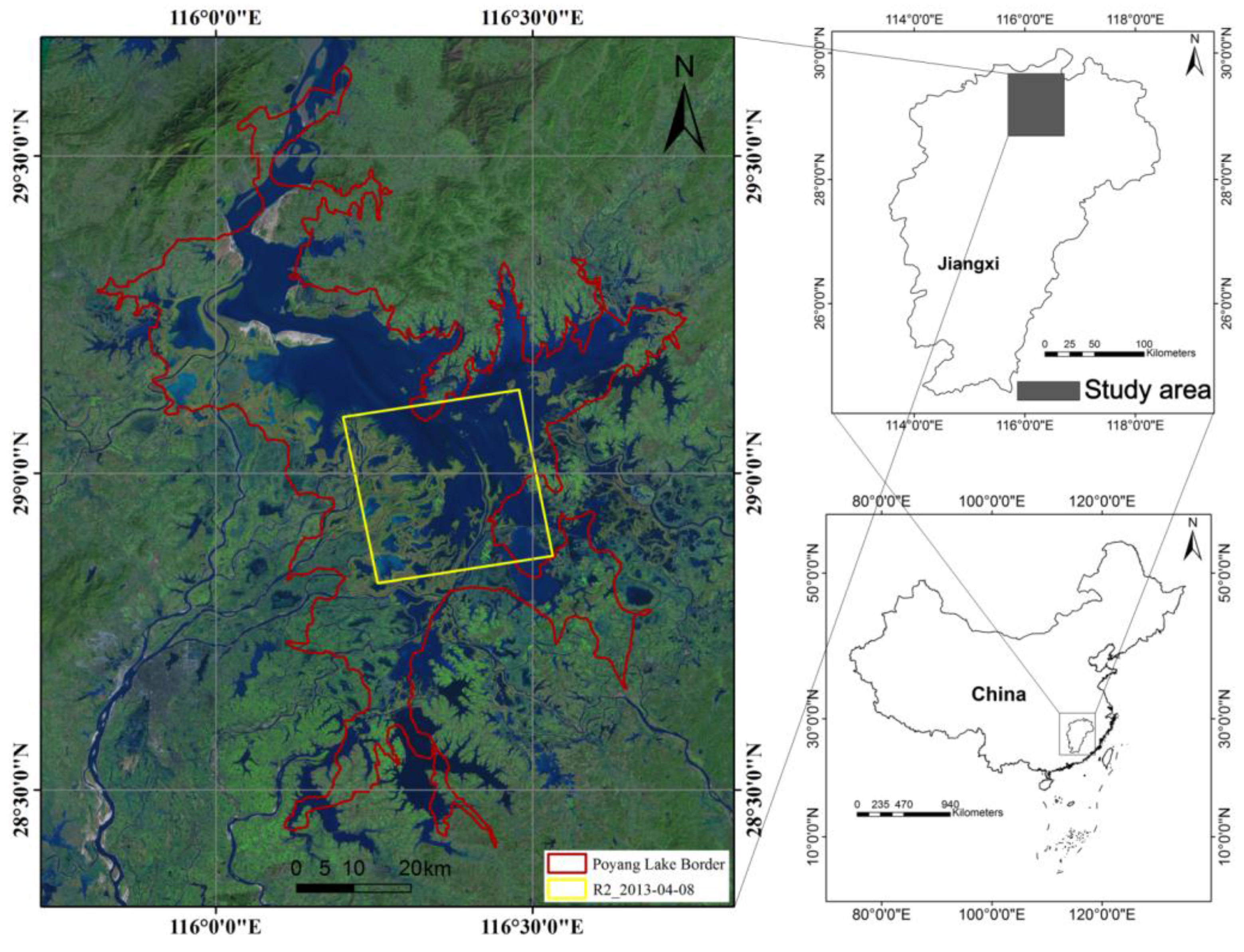
For wetland vegetation in the Poyang Lake area in Jiangxi, China, the modified MIMICS model and the rice scattering model (RSM) [22] developed by Cuizhen Wang were used to simulate the backscatter in the previous researches [17,18,20,21]. By ignoring the curvature of the blade and the strong coherence from the great density of grass, the simulation results of the two models have large error. In this paper, a coherent scattering model is developed for wetland vegetation in the Poyang Lake area in Jiangxi, China. The model presents realistic computer-generated vegetation structures, and accounts for the curvature of the leaf, lodging situation of the vegetation, and phase correlation between the plant components and different scattering mechanisms. In the calculation of soil surface scattering, the model combines the Advanced Integral Equation Model and Oh’s 2002 model [23,24] to provide more accurate simulations. The overall accuracy of the model is verified using C-band SAR data acquired by Radarsat-2. To reduce errors, Radarsat-2 SAR images of the Poyang Lake area were acquired concurrently with the collection of field data from the experimental area during April 2013.

In the next section, we discuss the collection of ground truth and field data, as well as the processing of the Radarsat-2 imagery. Section 3 describes the generation of the geometric structure of vegetation and the simulation of the Poyang Lake wetland. A description of the theory behind the model is also included. Section 4 discusses the validity of the model and Section 5 presents the results from a sensitivity analysis, before all results are summarized in the final section.

2. Study Area and Data

2.1. Test Site

The study site is located in the Poyang Lake Wetland in Jiangxi Province, China (28°22′N–29°15′N, 115°47′E–116°45′E), as shown in Figure 1. Poyang Lake is an internationally important wetland and the largest freshwater lake in China. The climate is characterized as a subtropical, humid monsoon climate with a mean annual precipitation of 1620 mm and an average annual temperature of about 17 °C. The hydrological environment of the Poyang Lake Wetland is very suitable for wetland vegetation. In the dry season (November–April), wetland vegetation emerges above water and starts to grow rapidly from early spring, with the aboveground biomass reaching the highest level in April. In the wet season (June–September), wetland vegetation is flooded and hardly grows except at the lakesides with higher ground level. In November, the water recedes and vegetation growth recommences [21]. The predominant vegetation in the Poyang Lake is Carex cinerascens Kükenth, which accounts for over 80% of the vegetation coverage. The sites we selected for the validation were shown as the yellow border area in Figure 1. The wetland vegetation is uniform and homogenous without human influence, which makes it very suitable for the validation of the scattering model.

Figure 1. Geographical location of study area. The background image is a Landsat image composed by bands 4(R), 3(G), and 2(B) showing the study area.

Figure 1. Geographical location of study area. The background image is a Landsat image composed by bands 4(R), 3(G), and 2(B) showing the study area.

2.2. SAR Data

The SAR data used in this study to validate the model were acquired by the Canadian satellite Radarsat-2 with fine quad-polarization mode (hh, hv, vh, and vv). The data, for which the range and azimuth pixel spacings are both 4.7 m, were acquired on 8 April 2013, with an angle of incidence ranging from 41° to 43°. To obtain the radar backscatter coefficient, calibration of this image was performed using the NEST (Next ESA SAR Toolbox) radar data processing software developed by the European Space Agency.

2.3. Field Measurements

Field measurements concurrent with the SAR data acquisition were collected from 7 to 10 April 2013. During the field survey, aboveground vegetation was harvested from 0.5 × 0.5 m quadrants at 22 sampling points located in the central and western parts of Poyang Lake. The leaf and stem characteristics, soil parameters, weight of grass, and location of the sampling point (obtained from GPS records) were recorded. The collected grasses were placed in an oven and dried for 12 h at a constant temperature (100 °C), following which the dry biomass was obtained. The permittivity of the grass was calculated using measurements of the grass moisture. In this paper, to facilitate processing, no distinction was made between stems and leaves in the calculation of the dielectric constant because they have approximately the same biological components. The Poyang Lake Wetland is very flat and the soil moisture is very high. Some places are even covered by water. It is difficult to measure the surface roughness. Considering that Poyang Lake Wetland is similar to a rice field, the soil surface parameters are taken to be constant: 0.0015 m for the root mean square height and 0.2 m for the correlation length [22]. The average values of the parameters, as measured at the sample points on 7–10 April 2013, are shown in Table 1.

Table 1. * Ground truth for Poyang Lake area obtained 7–10 April 2013.

Parameter		Value	Units
Soil volumetric moisture		0.4712	na
Grass gravimetric moisture		0.73	na
Grass density		2050	m−2
Grass height		52.55	cm
Herbaceous phytomass		348.76	g/m2
Stem	Length	29.17	cm
	Diameter	2.66	mm
	Tilt angle	[0, 10]	Degrees
	Azimuthal angle	[0, 360]	Degrees
Leaf	Length	26.63	cm
	ρmin	9.38	cm
	ρmax	25.07	cm
	zmin	4.21	cm
	zmax	20.325	cm
	Width	4.10	mm
	Thickness	0.22	mm
	Tilt angle	[10, 25]	Degrees
	Azimuthal angle	[110, 290]	Degrees
Number of leaves per grass		4	na
Pure stem layer		0.1073	m

* ρ_min is the minimum value for the horizontal length of the leaf, ρ_max is the maximum value for the horizontal length of the leaf, z_min is the minimum value for the vertical length of the leaf, and z_max is the maximum value for the vertical length of the leaf; see Section 3.1.2.

Table 1. * Ground truth for Poyang Lake area obtained 7–10 April 2013.

Parameter		Value	Units
Soil volumetric moisture		0.4712	na
Grass gravimetric moisture		0.73	na
Grass density		2050	m−2
Grass height		52.55	cm
Herbaceous phytomass		348.76	g/m2
Stem	Length	29.17	cm
	Diameter	2.66	mm
	Tilt angle	[0, 10]	Degrees
	Azimuthal angle	[0, 360]	Degrees
Leaf	Length	26.63	cm
	ρmin	9.38	cm
	ρmax	25.07	cm
	zmin	4.21	cm
	zmax	20.325	cm
	Width	4.10	mm
	Thickness	0.22	mm
	Tilt angle	[10, 25]	Degrees
	Azimuthal angle	[110, 290]	Degrees
Number of leaves per grass		4	na
Pure stem layer		0.1073	m

* ρ_min is the minimum value for the horizontal length of the leaf, ρ_max is the maximum value for the horizontal length of the leaf, z_min is the minimum value for the vertical length of the leaf, and z_max is the maximum value for the vertical length of the leaf; see Section 3.1.2.

3. Model and Method

3.1. Vegetation Structure Modeling

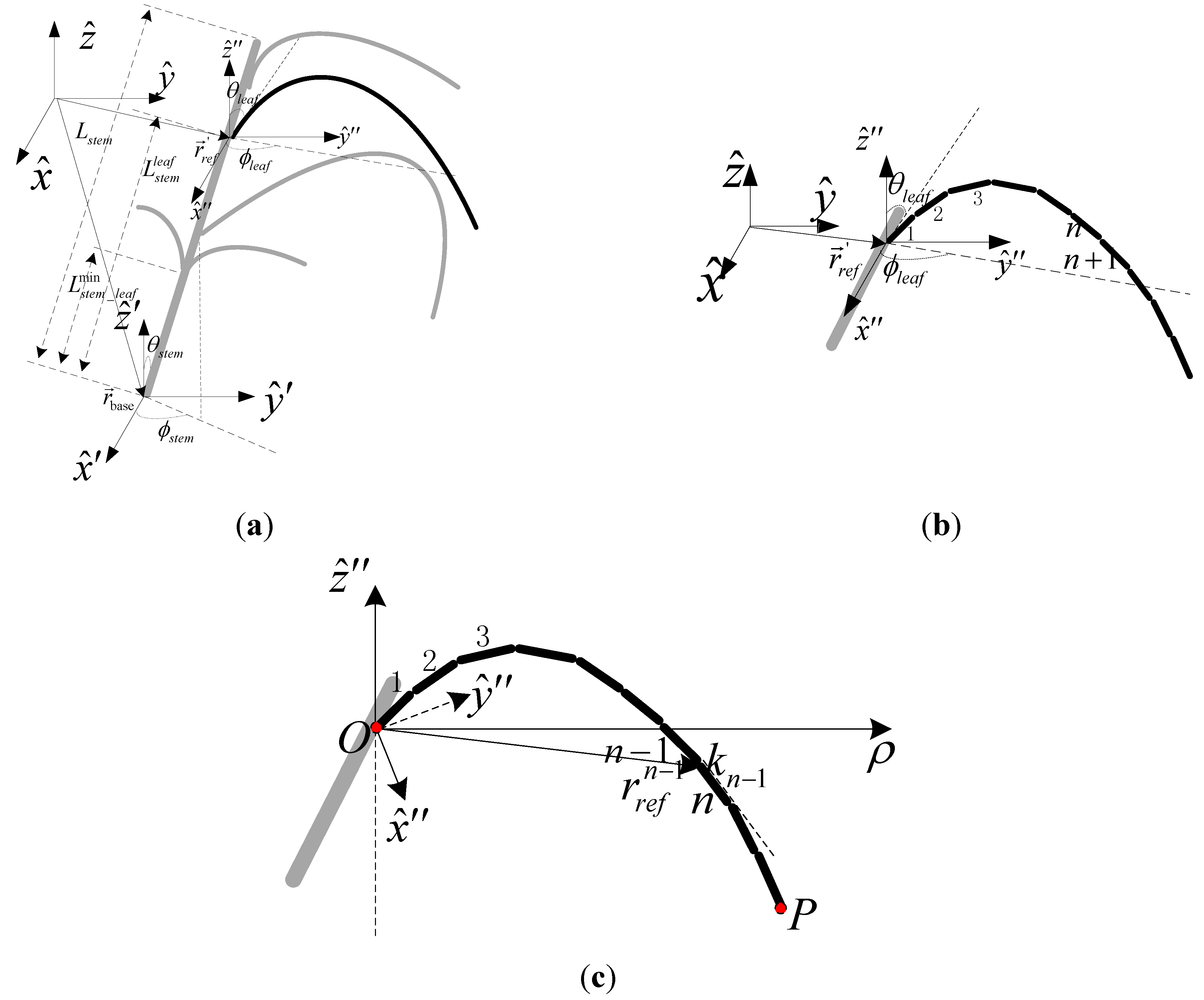
In order to ensure the accuracy of the scattering model, a virtual scene of the Poyang Lake Wetland and realistic three-dimensional vegetation structures were built. Botanical properties such as the branch dimension rules, leaf attachment, and curvature and size of blades had to be incorporated into the vegetation generation. Carex, which constitutes the main biomass in the Poyang Lake area, has a root-like stem and several curved blades. In the vegetation structure modeling, the stems were modeled as thin cylinders and the leaves represented as a combination of several thin cuboids placed end to end. The orientation angle of the cuboid was set by the plane angle and the angle of inclination of the section that the cuboid represented. The physiological parameters of the vegetation used in the botanical modeling were obtained from statistical analysis of the field measurements.

3.1.1. Generation of the Stem

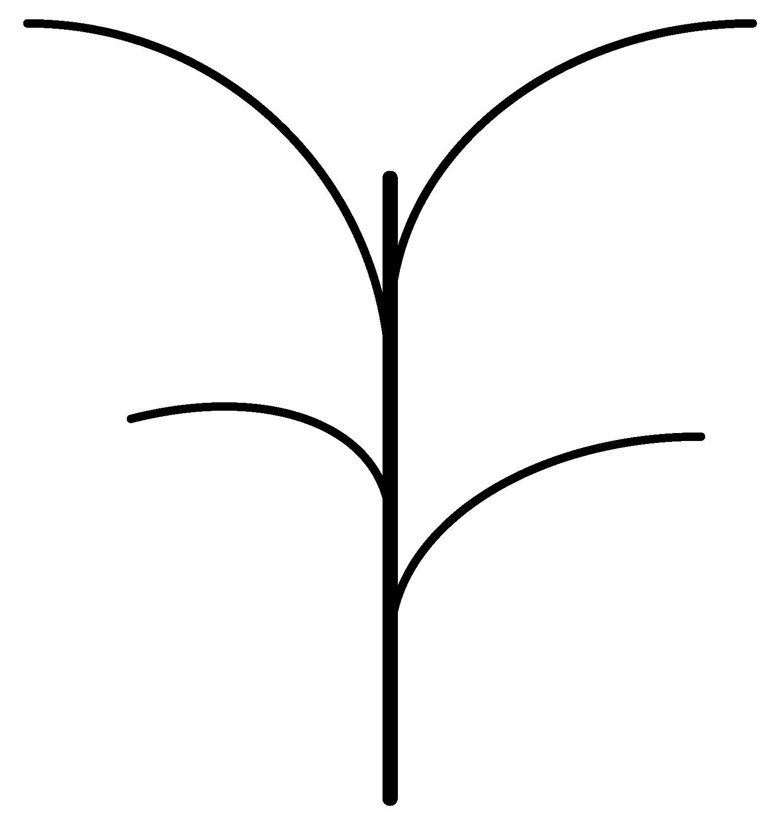
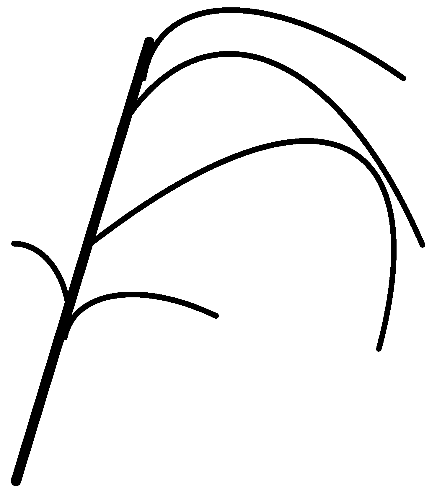
During the growth stage of Carex, its morphological characteristics change little but the sizes of the stems and leaves change considerably. Usually, the stems of Carex are almost perpendicular to the ground and the blades distributed within a range between a certain point on the stem and the top, as shown in Figure 2. However, the density of Carex increases greatly as it grows, and the plant is very likely to be affected by environmental factors such as wind. Therefore, Carex often exhibits a lodging situation, which results in most of the leaves pointing within a certain range (see Figure 3).

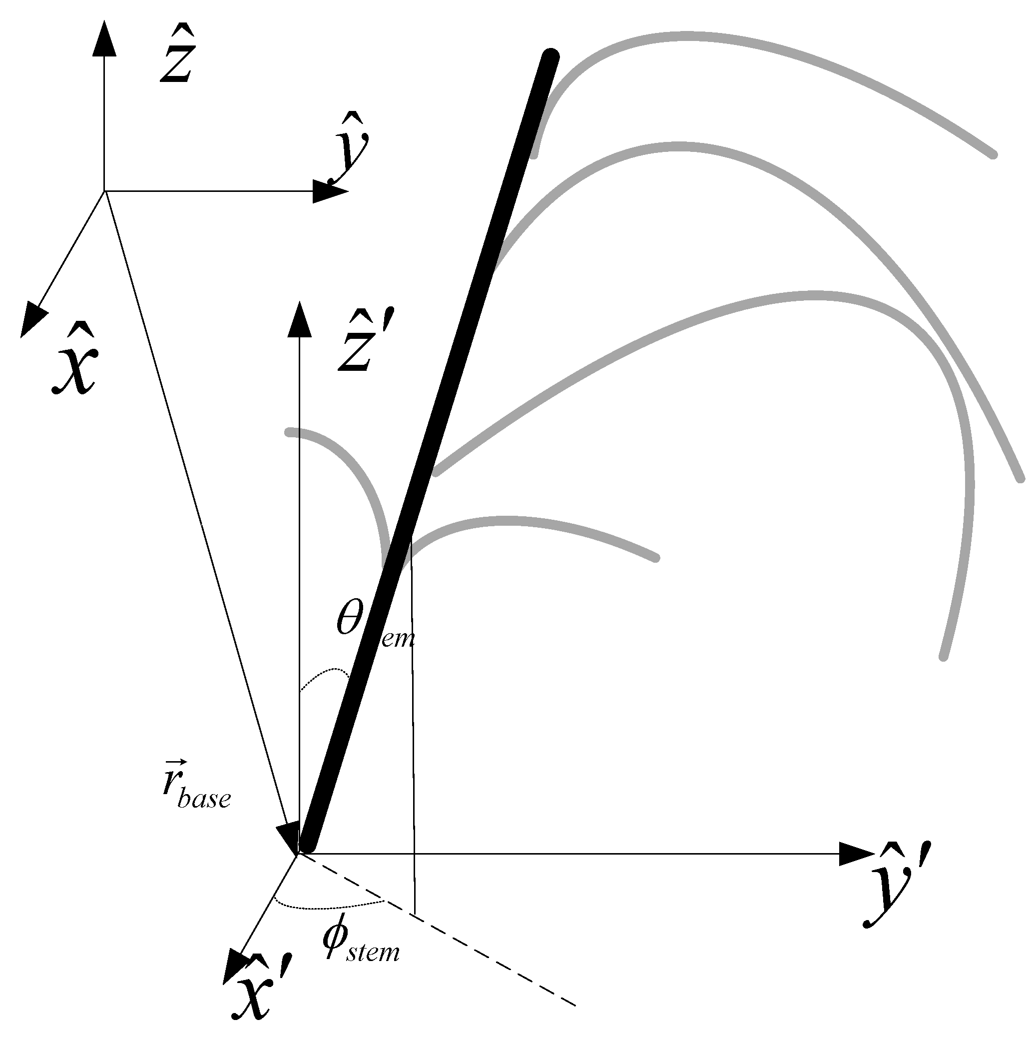
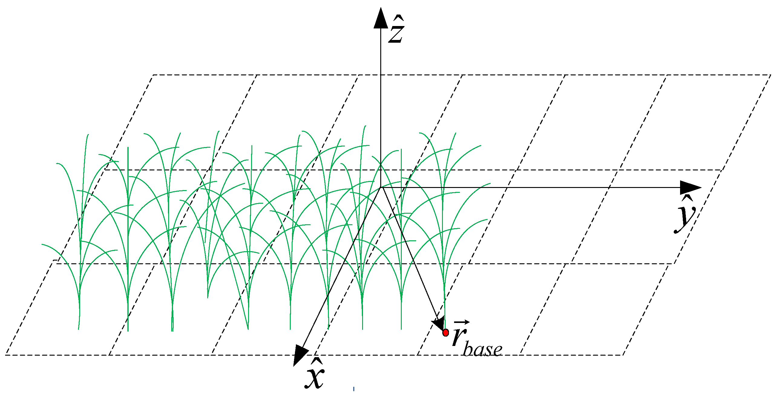
To facilitate the calculation of the phase correlation between the scattering from particles of different plants, all plants were placed within a three-dimensional coordinate system. In this study, the ground was considered flat because the Poyang Lake area is very flat. A global three-dimensional Cartesian coordinate system was used, which had its x–y plane parallel to the ground and the z-axis in the vertical direction was used. The locations of plants were generated randomly to form a uniform distribution according to the observed number density of Carex. Because the Carex in the Poyang Lake area are wild plants, they are not found growing in regularly spaced rows. The randomly generated plant locations were considered as the stem base points (Figure 4).

Taking the generated base point as the origin of the coordinate system, a local coordinate system parallel to the global coordinate system was then built and the stems generated, as shown in Figure 5. In this paper, the stems are represented as cylinders and a Carex plant is considered to consist of a single stem only and several leaves.

Figure 2. Picture of Carex under normal circumstances.

Figure 2. Picture of Carex under normal circumstances.

Figure 3. Picture of Carex in the lodging situation.

Figure 3. Picture of Carex in the lodging situation.

Figure 4. Picture of randomly distributed Carex.

Figure 4. Picture of randomly distributed Carex.

Figure 5. Stem generation and geometry of the stem model.

Figure 5. Stem generation and geometry of the stem model.

The contour vector for a stem can be described as

$${\overrightarrow{r}}_{stem}=l_{stem}\sin {\text{θ}}_{stem}\cos {\text{ϕ}}_{stem}\widehat{x}+l_{stem}\sin {\text{θ}}_{stem}\sin {\text{ϕ}}_{stem}\widehat{y}+l_{stem}\cos {\text{θ}}_{stem}\widehat{z}+{\overrightarrow{r}}_{base}$$

(1)

In Equation (1), 0 ˂ l_stem ≤ L_stem, L_stem is the length of the stem, θ_stem is the tilt angle of the stem, and ${\varnothing }_{stem}$ is the azimuth angle. The distribution and range of the tilt angle and azimuth angles were obtained from ground truth data and the angle values generated by the Monte Carlo simulation.

3.1.2. Generation of Leaf

The leaves of Carex in the Poyang Lake area are long and narrow. The curvature of the leaves can be approximated by a quadratic curve and their cross section is rectangular. In this coherent scattering model, the Carex leaf is represented as a combination of several thin cuboids placed end to end. The orientation angle of a cuboid is set by the plane angle and the inclination angle of the section that the cuboid represents (Figure 6).

The leaves of Carex are located directly at the stem in contrast to the random locations of the Carex canopy. In a Carex plant, the bases of the leaves are distributed uniformly within a certain range of the stem. Generally, the tilt angles of the leaves are not fixed and decrease consistently from the stem root to the stem tip. For a single leaf, the inclination angles of the cuboids are not fixed and increase from the leaf root to the leaf tip. The contour vector of the first cuboid connected to the blade base point is expressed as follows:

$${\overrightarrow{r}}_{leaf}^1=l_1\sin {\mathrm{\theta }}_{leaf}^0\cos {\mathrm{\varphi }}_{leaf}\widehat{x}+l_1\sin {\mathrm{\theta }}_{leaf}^0\sin {\mathrm{\varphi }}_{leaf}\widehat{y}+l_1\cos {\mathrm{\theta }}_{leaf}^0\widehat{z}+r_{ref}^{\prime }$$

(2)

where, l₁ is the length element, ${\varnothing }_{leaf}$ is the leaf azimuth angle ${\mathrm{\theta }}_{leaf}^0={\mathrm{\theta }}_{leaf}$, ${\mathrm{\theta }}_{leaf}^0$ denotes the tilt angle of the first cuboid, θ_leaf is the tilt angle of the leaf, and $r_{ref}^{\prime }$ specifies the node where a leaf is attached to the stem. $r_{ref}^{\prime }$ can be written as

$$r_{ref}^{\prime }=L_{stem}^{leaf}\sin {\displaystyle \int }{\mathrm{\theta }}_{stem}\cos {\mathrm{\varphi }}_{stem}\widehat{x}+L_{stem}^{leaf}\sin {\displaystyle \int }{\mathrm{\theta }}_{stem}\sin {\mathrm{\varphi }}_{stem}\widehat{y}+L_{stem}^{leaf}\cos {\displaystyle \int }{\mathrm{\theta }}_{stem}\widehat{z}+{\overrightarrow{r}}_{base}$$

(3)

where θ_stem and ${\varnothing }_{stem}$represent the tilt and azimuthal angles of the stem, respectively. ${\overrightarrow{\text{r}}}_{base}$ specifies the base point of the stem, and $L_{stem}^{leaf}$ represents the distance from the base point of the stem to the node where a leaf is attached to the stem.

Figure 6. Grass structure with discrete leaves. (a) geometry of the blade, (b) base point of the first cuboid, and (c) base point of the n-th cuboid.

Figure 6. Grass structure with discrete leaves. (a) geometry of the blade, (b) base point of the first cuboid, and (c) base point of the n-th cuboid.

The next step is to build a local two-dimensional coordinate system in the plane where the single leaf is located, as shown in Figure 6c. The junction between the leaf and the stem is taken as the origin (O) and point P (ρ_M, z_M) represents the leaf tip. ρ_min ≤ ρ_M ≤ ρ_max, and z_min ≤ z_M ≤ z_max where ρ_min is the minimum value for the horizontal length of the leaf, ρ_max is the maximum value for the horizontal length of the leaf, Z_min is the minimum value for the vertical length of the leaf and z_max is the maximum value for the vertical length of the leaf. ρ_min, ρ_max, z_min, and z_max were obtained from the statistical analysis of the ground data. The curvature of the blade can be given as

$$z=f(\text{ρ})=\frac{z_M-\tan {\mathrm{\theta }}_{leaf}\times {\text{ρ}}_M}{{{\text{ρ}}_M}^2}\times {\text{ρ}}^2+\tan {\mathrm{\theta }}_{leaf}\times \text{ρ}$$

(4)

where $\text{ρ}\in \left[0,{\text{ ρ}}_M\right]$ and the leaf is divided equally into N parts in the direction of the ρ-axis. The ρ coordinate of the left endpoint of the n-th cuboid (which is also the right endpoint of the (n-1)-th cuboid) is $\frac{{\text{ρ}}_M}{N}·\left(n-1\right)$. The slope of the n-th cuboid can be represented as

$$k_{n-1}=f^{\prime }(\mathrm{\rho }=\frac{{\mathrm{\rho }}_M}{N}\times (n-1))=\frac{2(n-1)\times (z_M-\tan {\mathrm{\theta }}_{leaf}\times {\mathrm{\rho }}_M)}{N\times {{\mathrm{\rho }}_M}^2}+\tan {\mathrm{\theta }}_{leaf}$$

(5)

The length of the n-th cuboid is defined as

$$L_n=\sqrt{1+{k_{n-1}}^2}\times \frac{{\mathrm{\rho }}_M}{N}$$

(6)

The contour vector of the nth cuboid can be described by

$${\overrightarrow{r}}_{leaf}^n=l_n\sin {\mathrm{\theta }}_{leaf}^{n-1}\cos {\mathrm{\varphi }}_{leaf}\widehat{x}+l_n\sin {\mathrm{\theta }}_{leaf}^{n-1}\sin {\mathrm{\varphi }}_{leaf}\widehat{y}+l_n\cos {\mathrm{\theta }}_{leaf}^{n-1}\widehat{z}+r_{ref}^{n-1}$$

(7)

In Equation (8), l_n is the length element, $l_n\in \left[0, L_n\right]$, ${\mathrm{\varphi }}_{leaf}$ is the azimuthal angle, ${\mathrm{\theta }}_{leaf}^{n-1}$ is the tilt angle of the n-th cuboid, ${\mathrm{\theta }}_{leaf}^{n-1}=\arctan k_{n-1}$, ${\mathrm{\theta }}_{leaf}^0={\mathrm{\theta }}_{leaf}$, and $r_{ref}^{n-1}$ represents the node between the n-th cuboid and the (n − 1)-th cuboid. The vector coordinate of $r_{ref}^{n-1}$ can be written as

$$r_{ref}^{n-1}=\frac{{\mathrm{\rho }}_M}{N}\times (n-1)\times \cos {\mathrm{\varphi }}_{leaf}\widehat{x}+\frac{{\mathrm{\rho }}_M}{N}\times (n-1)\times \sin {\mathrm{\varphi }}_{leaf}\widehat{y}+f(\mathrm{\rho }=\frac{{\mathrm{\rho }}_M}{N}\times (n-1))\widehat{z}$$

(8)

In Equation (9), $r_{ref}^0=r_{ref}^{\prime }$. Through the above analysis, the curvature of the leaves can be obtained. The number of segments (N) can be set according to the simulation accuracy and calculation speed. In the simulation process, the thickness and width of the blade are considered to be distributed uniformly.

3.2. Scattering Calculation

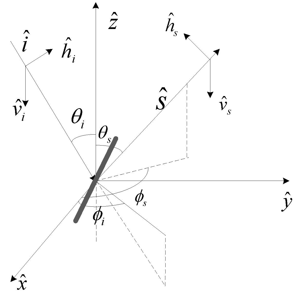
For all scatterers, the electromagnetic wave can be scattered as shown in Figure 7. Suppose a plane wave is illuminating the ground plane from the upper half-space. If k₀ is the wave number in free space, ${\widehat{k}}_i$ is the unit vector in the incident direction, and ${\widehat{q}}_i\left({\widehat{v}}_i,{\widehat{h}}_i\right)$ denotes the horizontal or vertical unit vector, the plane wave is then defined as follows:

$${\overrightarrow{E}}^i={\widehat{q}}_i{E}_0{e}^{j{k}_0{\widehat{k}}_i\cdot \overrightarrow{r}}$$

(9)

$${\widehat{k}}_i=\sin {\mathrm{\theta }}_i\cos {\mathrm{\varphi }}_i\widehat{x}+\sin {\mathrm{\theta }}_i\sin {\mathrm{\varphi }}_i\widehat{y}-\cos {\mathrm{\theta }}_i\widehat{z}$$

(10)

$${\widehat{h}}_i=\frac{\widehat{z}\times {\widehat{k}}_i}{|\widehat{z}\times {\widehat{k}}_i|}=-\sin {\mathrm{\varphi }}_i\widehat{x}+\cos {\mathrm{\varphi }}_i\widehat{y}$$

(11)

$${\widehat{v}}_i={\widehat{h}}_i\times {\widehat{k}}_i=-\cos {\mathrm{\theta }}_i\cos {\mathrm{\varphi }}_i\widehat{x}-\cos {\mathrm{\theta }}_i\sin {\mathrm{\varphi }}_i\widehat{y}-\sin {\mathrm{\theta }}_i\widehat{z}$$

(12)

For the scattered wave, ${\widehat{k}}_s$ is the unit vector in the scattering direction and ${\widehat{v}}_s$ and ${\widehat{h}}_s$ represent the horizontal and vertical unit vectors, respectively. The expressions for these vectors can be obtained in a similar way to those for ${\widehat{v}}_i$ and ${\widehat{h}}_i$.

$${\widehat{k}}_s=\sin {\mathrm{\theta }}_s\cos {\mathrm{\varphi }}_s\widehat{x}+\sin {\mathrm{\theta }}_s\sin {\mathrm{\varphi }}_s\widehat{y}+\cos {\mathrm{\theta }}_s\widehat{z}$$

(13)

Figure 7. Scattering of an electromagnetic wave by a dielectric scatterer.

Figure 7. Scattering of an electromagnetic wave by a dielectric scatterer.

3.2.1. The Model for a Single Scatterer

For Poyang Lake Carex, the single-scatterer model consists principally of a stem model and a leaf model. Although an exact scattering solution does not exist for cylinders of finite length, an approximate solution can be used, which assumes that the internal field induced within a finite cylinder is the same as that for an infinite cylinder with the same cross section and dielectric constant. In the simulation of Carex leaves, the situation is similar to that for the leaves of most low crops, i.e., the minimum size of the leaves (d) can meet the condition $k_{0}d\left(\sqrt{{\text{ε}}_r}-1\right)\ll 1$ in the microwave band, where k₀ is the wave number in free space and ε_r is the effective dielectric constant. Therefore, the electromagnetic field scattered by the leaves can, therefore, be calculated using the generalized Rayleigh–Gans approximation [25].

3.2.2. Scattering Formulations for Carex in the Poyang Lake Wetland

To the first order of approximation, the scattering from a Carex plant can be approximated by the superposition of the scattered electromagnetic field from each scatterer within the Carex structure. Hence, neglecting the effect of multiple scattering between the scatterers, the total scattered field from a single Carex can be evaluated as

$$E^s=\frac{e^{jkr}}{r}{\displaystyle \sum _{n=1}^N{e}^{i{\mathrm{\varphi }}_n}{S}_n}\times E_0^i$$

(14)

In Equation (14), N is the total number of scatterers within a Carex structure and S_n is the scattering matrix of the n-th scatterer above a dielectric plane. ${\mathrm{\varphi }}_n$ is a phase compensation term that accounts for the shift of the phase reference from the local coordinate system of the n-th scatterer to the global coordinate phase reference. ${\mathrm{\varphi }}_n$ depends on the position (r_n) of the n-th scatterer in the global coordinate system, and ${\mathrm{\varphi }}_n$ is given by

$${\mathrm{\varphi }}_n=({\widehat{k}}_i-{\widehat{k}}_s)\times {\overrightarrow{r}}_n$$

(15)

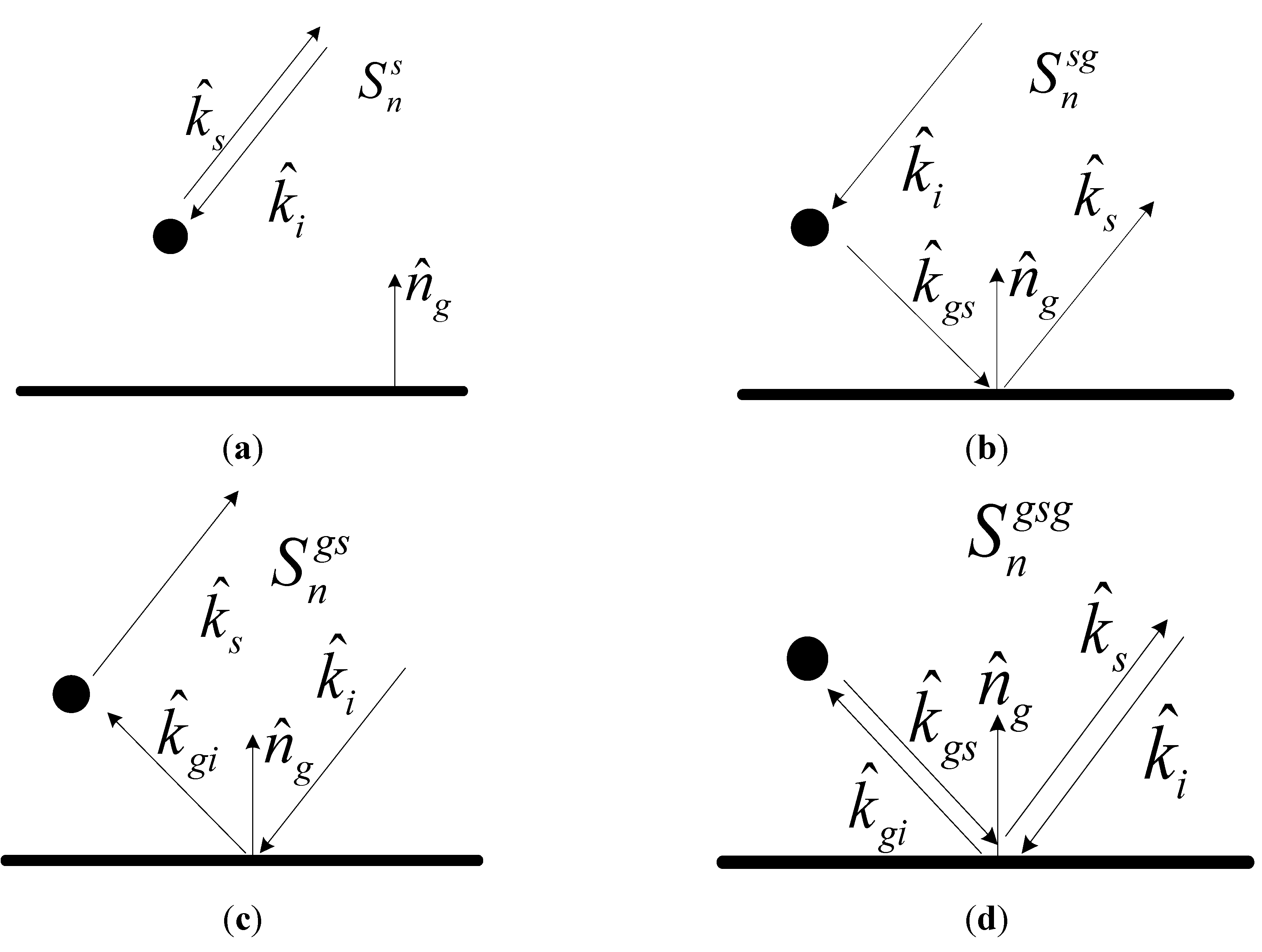
For each scatterer in the Carex structure, in order to compute the local scattering matrix (S_n), several scattering mechanisms are considered as the scattering model. Figure 8 depicts four different mechanisms, including:

(1)

direct scattering from vegetation particles ($S_n^S$);

(2)

scatterer-ground scattering ($S_n^{Sg}$);

(3)

ground-scatterer scattering ($S_n^{gS}$);

(4)

ground-scatterer–ground scattering ($S_n^{gSg}$).

Figure 8. Four scattering mechanisms (a–d).

Figure 8. Four scattering mechanisms (a–d).

The scattering matrix (S_n) can be written in terms of its components as

$$S_n=S_n^s+S_n^{gs}+S_n^{sg}+S_n^{gsg}$$

(16)

where

$$S_n^s=S_n^0({\widehat{k}}_s,{\widehat{k}}_i)$$

(17)

$$S_n^{sg}=e^{j{\tau }_s}R({\widehat{k}}_s,{\widehat{k}}_{gs})\times S_n^0({\widehat{k}}_{gs},{\widehat{k}}_i)$$

(18)

$$S_n^{gs}=e^{j{\tau }_i}{S}_n^0({\widehat{k}}_s,{\widehat{k}}_{gi})\times R({\widehat{k}}_{gi},{\widehat{k}}_i)$$

(19)

$$S_n^{gsg}=e^{j({\tau }_i+{\tau }_s)}R({\widehat{k}}_s,{\widehat{k}}_{gs})\times S_n^0({\widehat{k}}_{gs},{\widehat{k}}_{gi})\times R({\widehat{k}}_{gi},{\widehat{k}}_i)$$

(20)

and

$${\widehat{k}}_{gi}={\widehat{k}}_i-2{\widehat{n}}_g({\widehat{n}}_g\times {\widehat{k}}_i)$$

(21)

$${\widehat{k}}_{gs}={\widehat{k}}_s-2{\widehat{n}}_g({\widehat{n}}_g\times {\widehat{k}}_s)$$

(22)

$${\tau }_i=2k_0({\overrightarrow{r}}_n\times {\widehat{n}}_g)({\widehat{n}}_g\times {\widehat{k}}_i)$$

(23)

$${\tau }_s=2k_0({\overrightarrow{r}}_n\times {\widehat{n}}_g)({\widehat{n}}_g\times {\widehat{k}}_s)$$

(24)

In Equations (17)–(20), $S_n^0$ is the bistatic scattering matrix of the n-th scatterer in free space. The parameters in brackets denote the unit vectors in the incident and scattering directions. In the above expressions, ${\widehat{n}}_g$ is the unit vector, normal to the ground surface. The phase terms, τ_i and τ_s, account for the extra path lengths of the image excitation and the image scattered waves, respectively. R is the reflection matrix of the dielectric plane, whose elements are derived in terms of the Fresnel reflection coefficients. In the model, the multiple scattering among vegetation was neglected for the following reasons:

(1)

The reasonable simulation results were obtained with the current models of rice field, in which the multiple scattering among vegetation did not be considered [26,27]. The structure, condition and the ground surface of Poyang Lake wetland vegetation are similar to rice, so the multiple scattering among vegetation is also neglected in our manuscript.

(2)

Because the curved blades was used for the discrete method, it is very complex if we considered the multiple scattering among vegetation, and the near-field scattering for two curved blades had not ever been developed in the current studies. It is a difficult problem for developing the related model. If discretizing the blades first and calculating the multiple scattering among vegetation, the model was time consuming very much with Monte Carlo simulation. In order to simplify the model and facilitate the inversion of the biophysical parameters, the multiple scattering among vegetation was negligible.

3.3. Attenuation Calculation

The above analysis is not quite complete because in the calculation of scattering from the n-th scatterer, the other scatterers are considered non-existent. However, the effect of the attenuation and phase change of the coherent wave propagating in the random media can be readily modeled by calculating the mean field within the random medium.

For sparse media such as vegetation, Foldy’s approximation can be employed to account for the effects of absorption and scattering on a coherent wave caused by the inhomogeneities in a random medium. The propagation of a coherent wave is governed by the following Equation under Foldy’s approximation:

$$\frac{dE}{ds}=iK\times E$$

(25)

where s is the distance along the propagation direction and

$$K=[\begin{array}{cc}{k}_0+M_{vv}& M_{vh}\\ M_{hv}& k_0+M_{hh}\end{array}]$$

(26)

$$M_{jl}=\frac{2\pi n_0}{k_0}<S_{jl}^0(\widehat{k},\widehat{k})>$$

(27)

where, k₀ is the wave number in free space, n₀ is the volume density of the scatterer, $S_{jl}^0\left(\widehat{k},\widehat{k}\right)$ is the forward scattering matrix (j and l can be v or h), and the symbol < > denotes the statistical average over the size and orientation angles. Equation (25) can be solved to give

$$E(s)=e^{-j{k}_{0}s}T(s,\widehat{k})\times E^0$$

(28)

where E⁰ is the field at s = 0 and T is the transmissivity matrix accounting for the extinction due to scattering and absorption. Statistically, the canopy structure exhibits azimuthal symmetry and therefore, there is no coupling between the horizontal and vertical components of the coherent field. Thus,

$$T=[\begin{array}{cc}{e}^{-j{M}_{vv}s}& 0\\ 0& e^{-j{M}_{hh}s}\end{array}]$$

(29)

The attenuation of the coherent wave is accounted for by the imaginary parts of M_hh and M_vv. Equation (29) is able to take into account the phase shift before and after the wave is scattered by a particular vegetative element.

In order to consider wave extinction in the scattering model, in this paper, the entire Carex structure is considered embedded within an effective medium with an effective propagation constant given by (26). Equations (17)–(20), for the components of the n-th scattering matrix, can be modified as follows:

$$S_n^s=T_n^i\times S_n^0({\widehat{k}}_s,{\widehat{k}}_i)\times T_n^i$$

(30)

$$S_n^{sg}=e^{j{\tau }_s}{T}_n^i\times R({\widehat{k}}_s,{\widehat{k}}_{gs})\times T_n^r\times S_n^0({\widehat{k}}_{gs},{\widehat{k}}_i)\times T^t$$

(31)

$$S_n^{gs}=e^{j{\tau }_i}{T}^t\times S_n^0({\widehat{k}}_s,{\widehat{k}}_{gi})\times T_n^r\times R({\widehat{k}}_{gi},{\widehat{k}}_i)\times T_n^i$$

(32)

$$S_n^{gsg}=e^{j({\tau }_i+{\tau }_s)}{T}^t\times R({\widehat{k}}_s,{\widehat{k}}_{gs})\times T_n^r\times S_n^0({\widehat{k}}_{gs},{\widehat{k}}_{gi})\times T_n^r\times R({\widehat{k}}_{gi},{\widehat{k}}_i)\times T^t$$

(33)

where $T_n^i$, $T_n^r$ and T^t are the transmissivity matrices for the direct, reflected, and total traveling path, respectively, as shown in Figure 9.

Figure 9. Extinction of a coherent wave in random media.

Figure 9. Extinction of a coherent wave in random media.

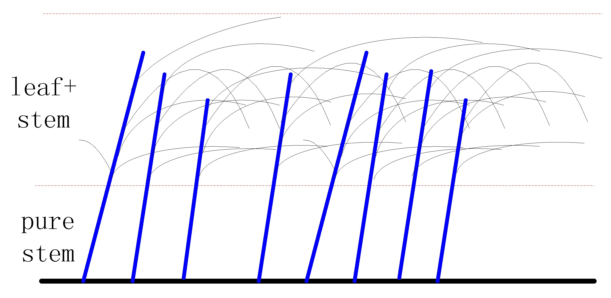
To account for non-uniform distributions of vegetation particle type and size in the direction of the vertical extent of most Carex, the random medium is divided into two layers: a pure stem layer and a mixed leaf and stem layer, as shown in Figure 10. Both layers, which have thicknesses d_m (m = 1, 2), are assumed parallel to the ground surface.

Figure 10. Layered Carex.

Figure 10. Layered Carex.

For the mixed leaf and stem layer, Equation (30) is modified as follows:

$$M_{jl}=\frac{2\pi }{k_0}[N_{stem}<S_{jl}^{stem}(\widehat{k},\widehat{k})>\text{+}{N}_{\text{leaf}}<S_{jl}^{leaf}(\widehat{k},\widehat{k})>]$$

(34)

where $\langle S_{jl}^{stem}\left(\widehat{k},\widehat{k}\right)\rangle$ and $\langle S_{jl}^{leaf}\left(\widehat{k},\widehat{k}\right)\rangle$ are the ensemble averages of the forward matrix for stems and leaves, respectively, in the mixed layer, and N_stem and N_leaf represent the volume densities of stems and leaves, respectively.

For each scatterer, the values of $T_n^i$ and $T_n^r$ should be calculated according to its position; the value of T^t is constant.

Attenuation at a given height is similar throughout any given vegetation layer; therefore, in the calculation process, the transmissivity matrices of particles at the same height are set to the same value in order to simplify the computation process by establishing a database of the transmissivity matrices.

3.4. Ground Scattering

Many classical methods describe microwave scattering by the ground. These include the Kirchhoff approximation for large-scale situations and the small perturbation model at smaller scales. The Kirchhoff model can be divided into two types: the geometrical optics model and physical optics model. However, all these models can only be used within a certain roughness range. The Integral Equation Model (IEM), which is based on the electromagnetic radiation transfer Equation and which was proposed by Fung et al. in 1992, has been widely used in microwave surface scattering simulations and analyses [28]. Chen et al. improved the IEM and developed the Advanced Integral Equation Model (AIEM), which can describe the scattering from smooth to rough surfaces [23]. The AIEM has been validated by Monte Carlo simulation and ground truth data, and it can be applied to surface scattering calculations with wide ranges of values of the dielectric constant, roughness, and frequency [29]. However, the calculated values for cross-polarization backscatter obtained using the AIEM are too low. In 1992 and 2002, Oh proposed two semi-empirical backscattering models based on the theoretical model and a large number of multi-angle polarimetric observations [24]. In Oh’s 2002 model, the relation involving the co-polarization ratio (p), cross-polarization ratio (q), surface soil moisture (Mv), roughness (surface RMS height (s), correlation length (l), and incident angle (θ) was established as:

$$p=1-{(\mathrm{\theta }/{90}^0)}^{0.35M{v}^{-0.65}}{e}^{-0.4{(ks)}^{1.4}}$$

(35)

$$q=0.1{(s/l+\sin 1.3\mathrm{\theta })}^{1.2}(1-e^{-0.9{(ks)}^{0.8}})$$

(36)

Experiments show that Oh’s 2002 model can be applied to a wide range of values of surface roughness, but the model has poor general applicability because of its many empirical components.

Based on the above analysis, the coherent scattering model for the Poyang Lake Wetland discussed in this paper calculates the co-polarized backscattering coefficient at the ground using the AIEM and it describes the cross-polarized backscattering coefficient using Oh’s 2002 model to simulate more accurately the ground scattering.

According to the above analysis, the backscatter simulation process for Poyang Lake can be expressed as follows. First, the locations of Carex plants are generated randomly based on the observed number density of Carex. Next, the stem and leaves of each Carex plant are generated according to their size and angle distributions. Thus, the vegetation database is then built. The canopy height is discretized into two layers, the extinction coefficient of each layer computed, and the database of transmissivity matrices established. The scattering matrix of individual Carex plants is calculated using Equations (30)–(33) and the scattered fields from all Carex plants are added coherently. The coefficient for backscattering from Carex plants can be expressed as:

$${\sigma }_{pq}^0=\frac{4\pi r^2}{A}·\frac{<|E_q^s{|}^2>}{|E_p^i{|}^2}$$

(37)

Finally, the field produced by ground scattering computed. By superimposing the effect of the attenuation by the Carex canopy, the backscattering coefficient of the ground is obtained. The backscattering coefficient for the Poyang Lake Wetland is then computed by adding incoherently the contributions of the Carex and ground:

$${\sigma }^0(\text{wetland})={\sigma }^0(Carex)+{\sigma }^0(\text{ground})$$

(38)

4. Results

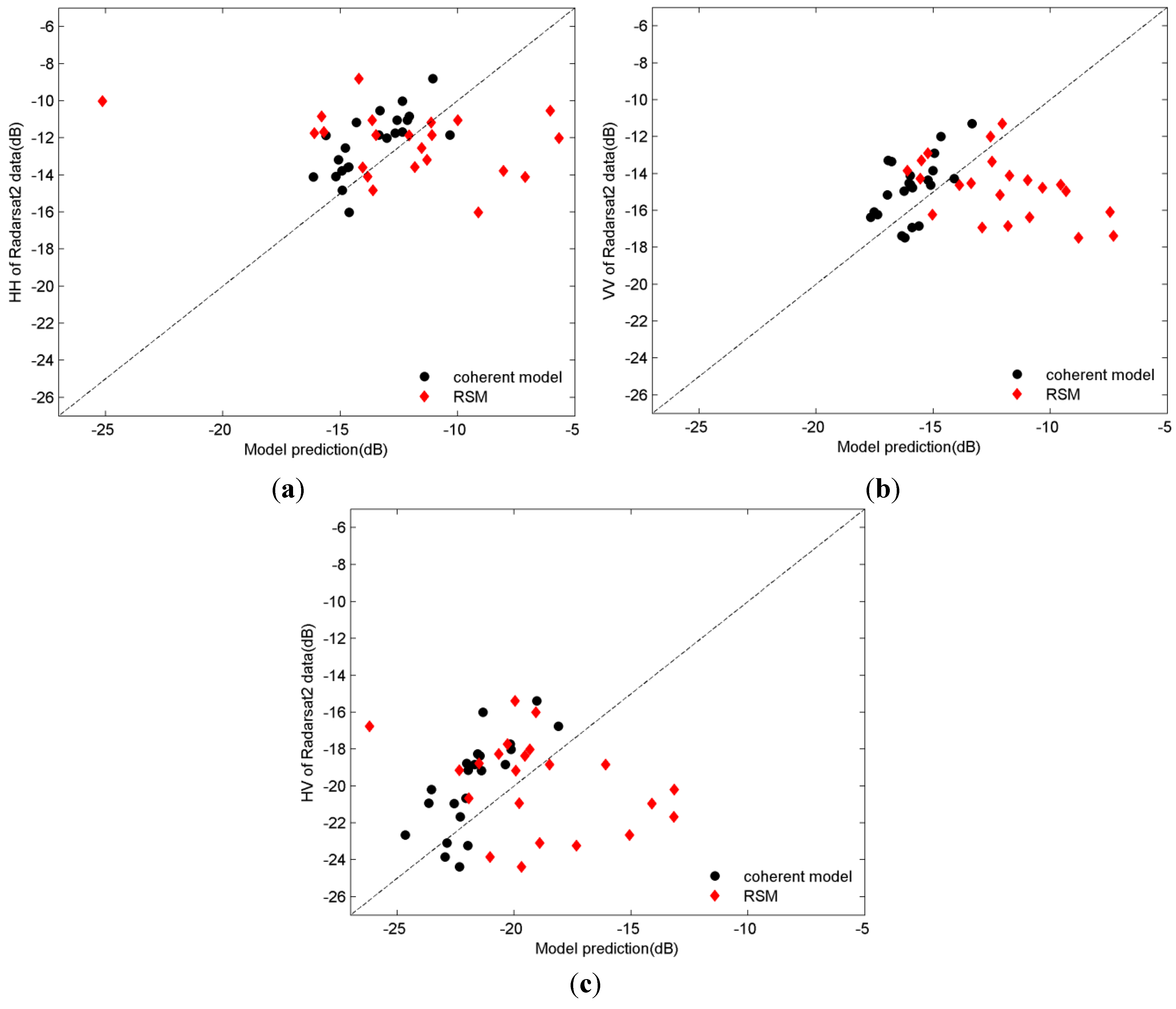
In this study, the coherent scattering model is developed for simulating the backscatter coefficient of wetland vegetation, and the model presents the realistic computer-generated vegetation structures, and accounts for the curvature of the leaf, lodging situation of the vegetation, and phase correlation between the plant components and different scattering mechanisms. The model of vegetation scattering was validated using Radarsat-2 C-band data (22 sampling data sets), and the existing RSM was used to compare with the developed model. The RSM was used to describe the rice, whose structure is similar with Carex in Poyang Lake Wetland. In the RSM, the following features were considered: (1) leaves were treated as very long and narrow ellipses; (2) leaves often extend directly upward and a specific probability distribution function was needed to simulate leaf scattering properties; and (3) the ear layer was ignored. The input parameters of the two models are from field survey.

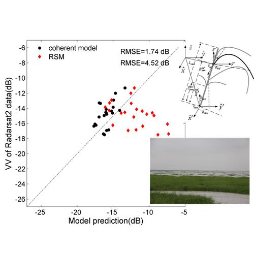
Figure 11 shows comparisons between the model predictions and measured backscattering coefficients throughout the study period for hh-, hv-, and vv-polarizations. It can be seen that the simulation results of the coherent scattering model are better than the RSM. The coherent scattering model has a root mean squared error (RMSE) of 1.82, 2.54, and 1.74 dB for hh-, hv-, and vv- polarizations, respectively, while the RSM has an RMSE of 4.90, 4.63, and 4.52 dB for hh-, hv-, and vv- polarizations, respectively (Table 2). In contrast to the RSM, the accuracy of the coherent scattering model is increased by approximately 2.5 dB. For the coherent model, there is good agreement for hh- and vv-polarizations. However, the results for hv-polarization are not particularly good. The differences between the coherent model and RSM results can be attributed to coherence effects due to the large density of grass and the curved blades.

Figure 11. Comparison between Radarsat-2 data and model prediction: (a) hh-polarization; (b) vv-polarization; and (c) hv-polarization.

Figure 11. Comparison between Radarsat-2 data and model prediction: (a) hh-polarization; (b) vv-polarization; and (c) hv-polarization.

Table 2. Validation of coherent model and rice scattering model (RSM).

Model Type	Polarization Type	RMSE/dB	Mean Ratio
Coherent model	hh	1.82	0.85
	hv	2.54	0.89
	vv	1.74	0.91
RSM	hh	4.90	0.78
	hv	4.63	0.78
	vv	4.52	0.69

Table 2. Validation of coherent model and rice scattering model (RSM).

Model Type	Polarization Type	RMSE/dB	Mean Ratio
Coherent model	hh	1.82	0.85
	hv	2.54	0.89
	vv	1.74	0.91
RSM	hh	4.90	0.78
	hv	4.63	0.78
	vv	4.52	0.69

Comparing the mean ratio of the estimated coefficients of these two models with the Radarsat-2 measured coefficient, both models have a value < 1. It can be seen that the two models underestimate the backscattering, although the underestimation of the coherent model was less than the RSM. These results can be attributed to the fact that both models ignored the multiple scattering between the vegetation scatterers, and the coherent model obtained better results because the coherence effect was considered. In contrast to the RSM, the mean ratio of the coherent scattering model is improved from 0.78, 0.78, and 0.69 (hh, hv, and vv, respectively) to 0.85, 0.89, and 0.91 (hh, hv, and vv, respectively).

5. Discussion

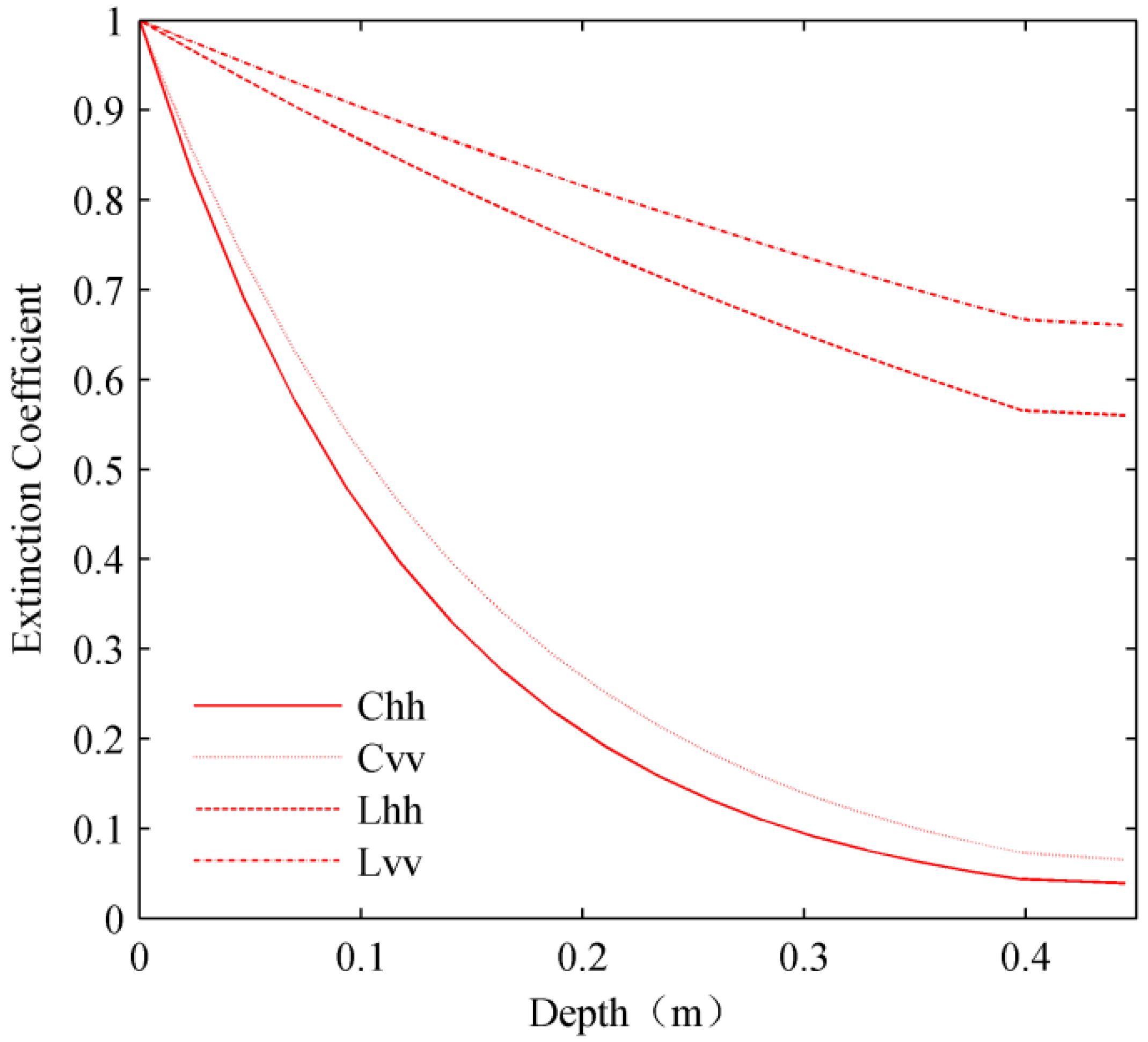
In this study, the coherent scattering model is developed for Poyang Lake wetland vegetation, and the precision of the model is improved compared to the existing model, although the simulation results are underestimated a little. In the following discussion, with the coherent scattering model, the attenuation, contribution from different scattering mechanisms, and the sensitivity of incident angle, leaf shape, the plant water content, soil volumetric moisture content, and grass number density are analyzed.

Figure 12 shows the extinction coefficient profile. In this graph, “depth” indicates the distance from the upper surface of the vegetation, and an extinction coefficient of “1” represents no attenuation, while a value of “0” represents complete attenuation. It should be noted that wave attenuation in the C-band is much greater than that in the L-band, which occurs because the lower the frequency of electromagnetic radiation, the stronger the penetration will be. It can also be seen that the extinction coefficient for horizontal polarization is greater than that for vertical polarization in both the C- and L-bands. In addition, the trend of the extinction coefficient with increasing depth is different in the two layers (the first layer, from 0 to 0.35 m, contains leaves and stems, while the second layer only contains stems). The amount of attenuation in the first layer is greater than in the second layer, which can be attributed to the high density of leaves in the first layer.

Figure 12. Extinction simulation for grass (incidence angle was 43°, frequencies were those of the C- and L-bands, and polarizations used were hh and vv).

Figure 12. Extinction simulation for grass (incidence angle was 43°, frequencies were those of the C- and L-bands, and polarizations used were hh and vv).

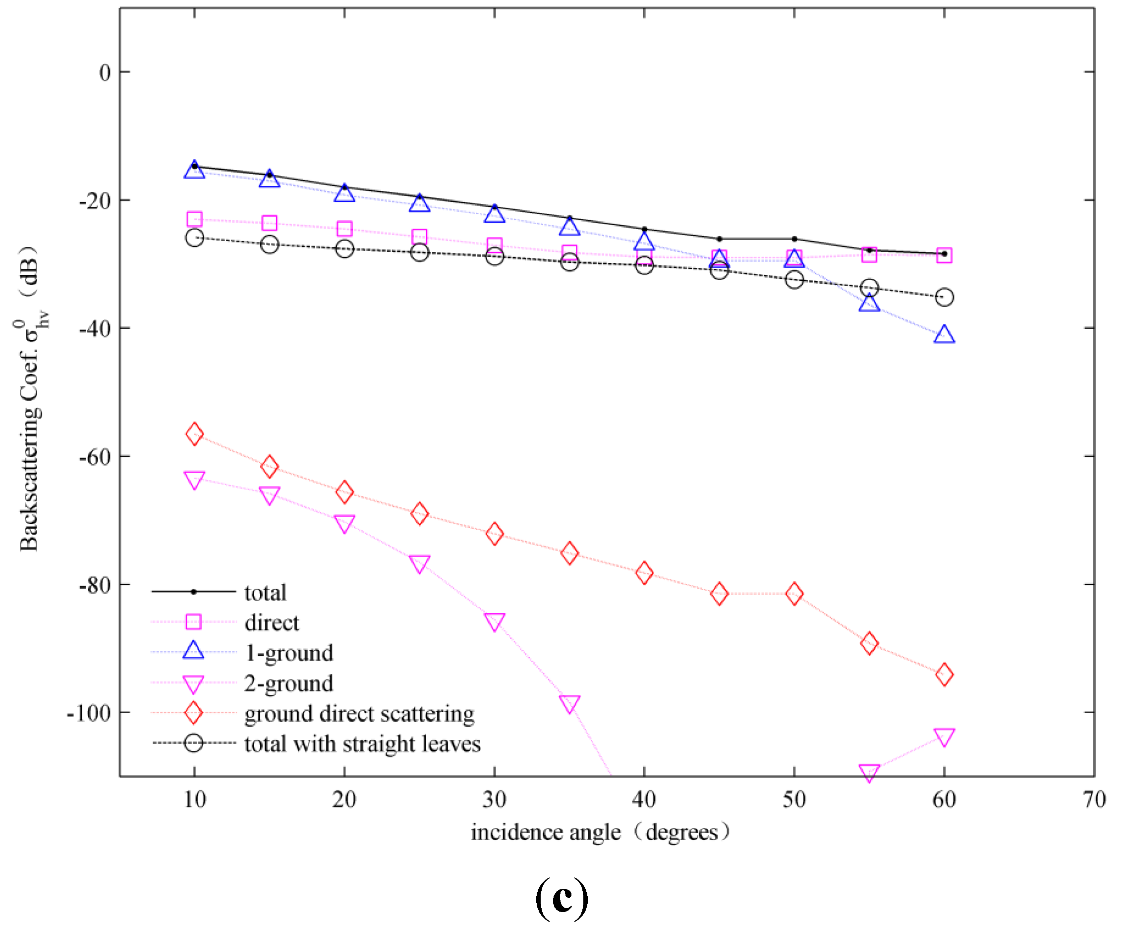
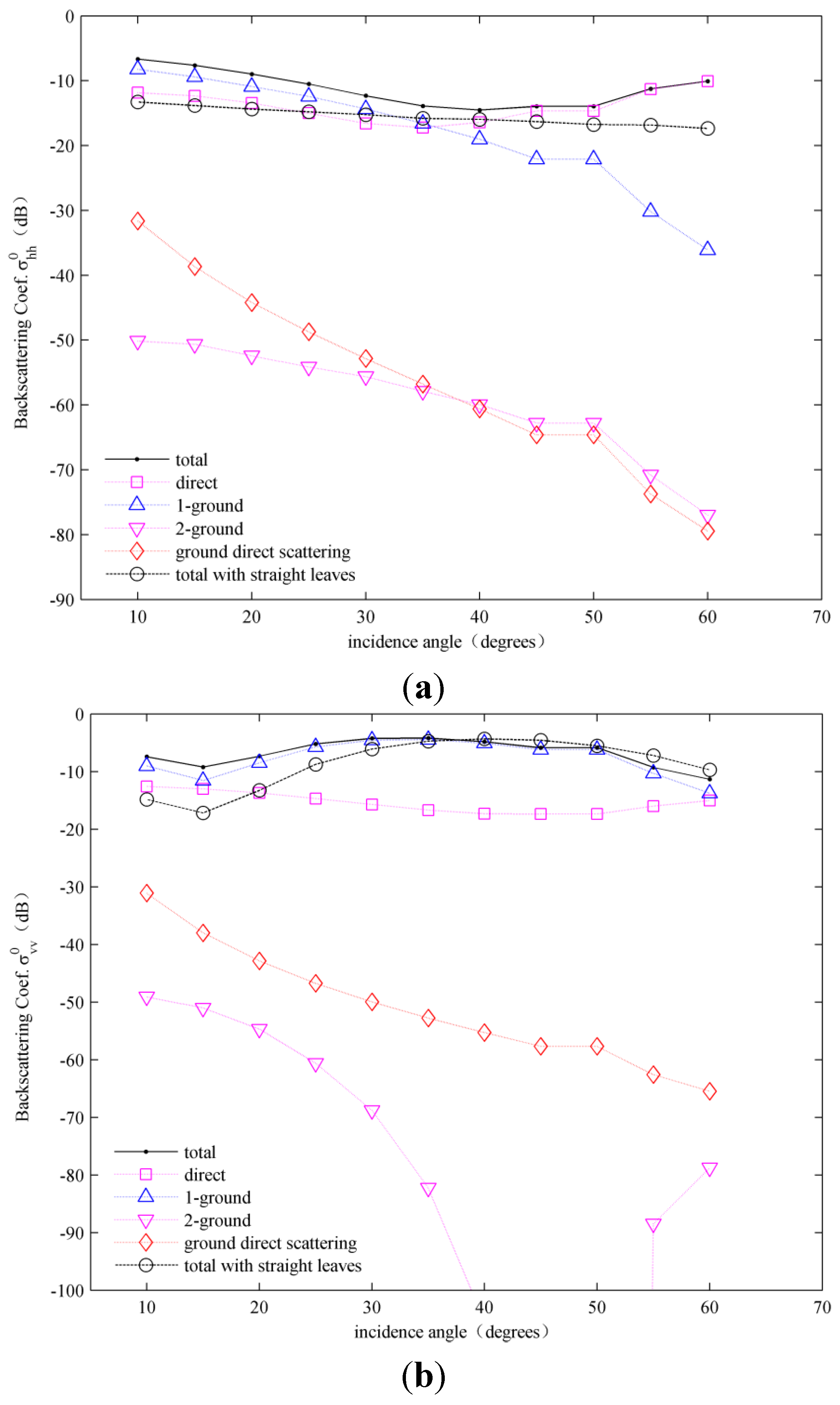
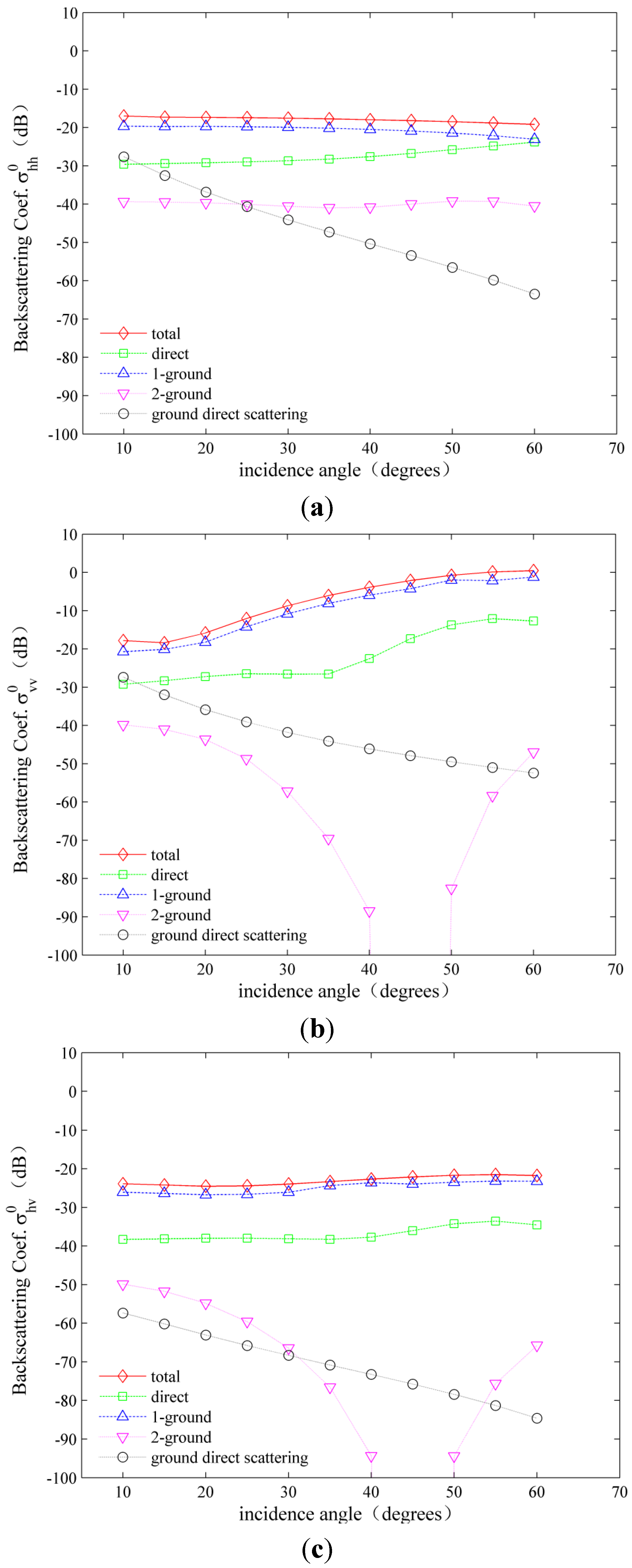
Figure 13 shows the simulated backscattering coefficient versus incidence angle for the C-band. The Monte Carlo simulations were performed at angles of incidence ranging from 10° to 60° in 5° increments. For hh-, vv-, and hv-polarizations, the two most significant components are the direct backscattering from vegetation and the single ground bounce (which includes scatterer-ground scattering and ground-scatterer scattering). For vv-polarization in particular, the single-ground-bounce mechanism dominates and its value is very close to the total scattering value. Furthermore, for vv-polarization, ground-scatterer-ground scattering is the least important mechanism, which is similar to the situation for hh- and hv-polarizations. This can be attributed to the large amount of attenuation in the C-band, see Figure 12. The amount of direct ground scattering is also small because of the attenuation and high soil moisture content. It is worth noting that for hh-polarization, when the incidence angle is <37°, the single ground bounce component is larger than the direct grass scattering component; however, for angles >37°, the situation is reversed. The same phenomenon also occurs for hv-polarization, but in this case, the critical angle is 43°.

Figure 13. Simulations of the angular variation of the scattering components in the C-band: (a) hh-polarization; (b) vv-polarization; and (c) hv-polarization (backscattering coefficient <−100 dB is not shown in the figure because of its minor contribution to total backscattering).

Figure 13. Simulations of the angular variation of the scattering components in the C-band: (a) hh-polarization; (b) vv-polarization; and (c) hv-polarization (backscattering coefficient <−100 dB is not shown in the figure because of its minor contribution to total backscattering).

Instead of using the leaf scattering model that considers curvature and the lodging situation, the data were again computed with leaves of the same width, thickness, and average length as before; however, this time, the leaves were assumed straight and the azimuthal angles assumed distributed uniformly. The simulated results are provided in Figure 13 (labeled “total with straight leaves”). It can be seen clearly that there are significant differences (as large as 4 dB) between the two total backscattering coefficients for the different leaf scattering models. Making the leaves straight and distributed uniformly not only changes the scattering attributed to the leaf elements but also to the scattering from stalks as well. This is because the attenuation is modified with the changes in modeled shape and distribution. This experiment indicates that considering the curvature and lodging situation of the leaves is critical for accurate modeling of grass.

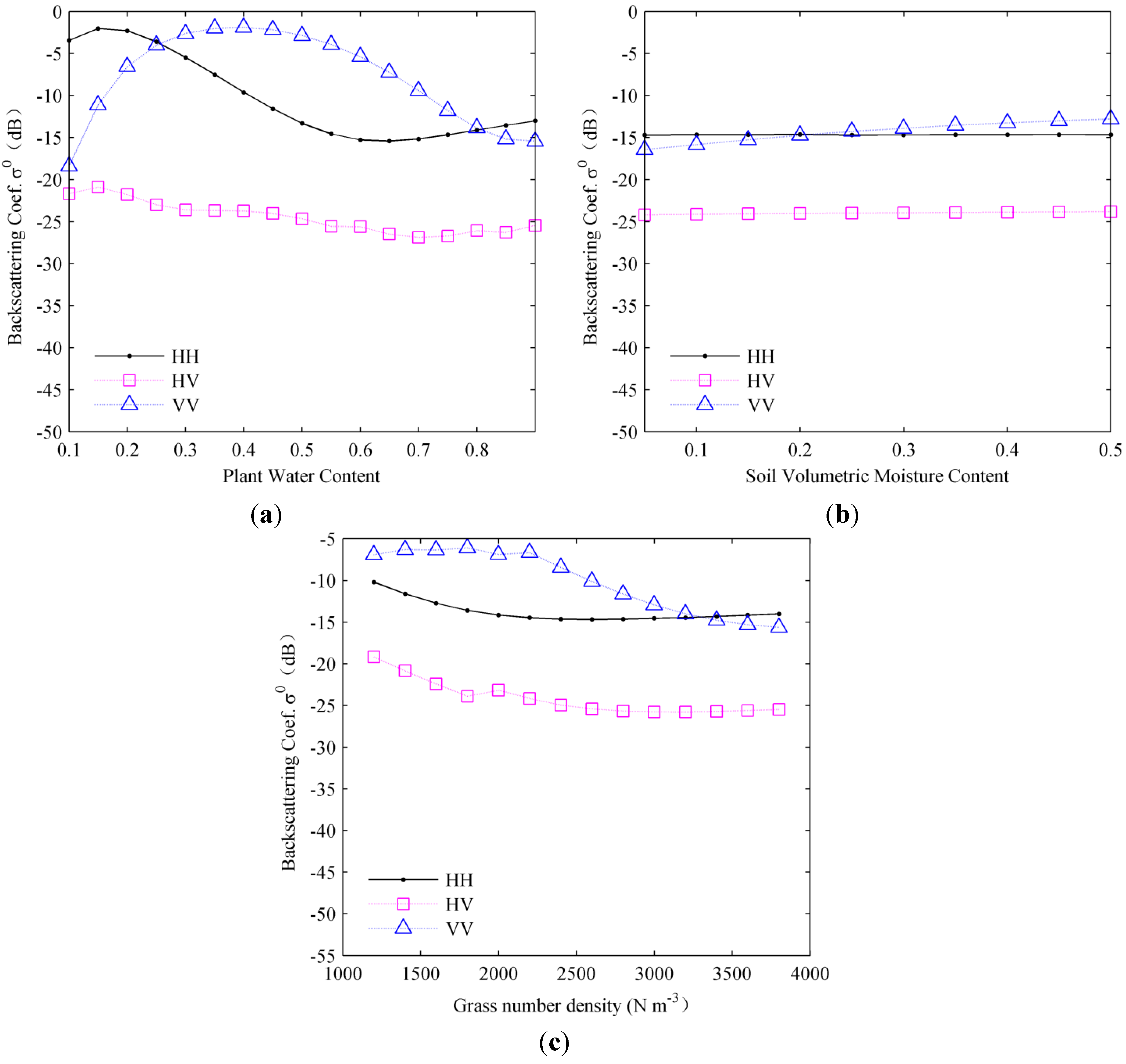
The results of an analysis of the sensitivity of the total backscattering coefficient to the plant water content, soil volumetric moisture content, and grass number density are shown in Figure 14. It can be seen from Figure 14a that for hh- and vv-polarizations, the plant water content is particularly sensitive to the backscatter coefficient. With the plant water content increasing, the value of the backscattering coefficient first increases then decreases, and the amount of variation can exceed 10 dB. In the C-band, the changes of soil volumetric moisture content have less impact on the total backscatter (Figure 14b). This can be attributed to the huge attenuation that results from the high density and depth of the wetland vegetation, and the consequent low penetration of C-band electromagnetic waves. Therefore, it can be concluded that the detection of soil surface moisture content in the Poyang Lake Wetland area using C-band radar is not feasible. Figure 14c shows that the backscattering either decreases slightly or remains stable with an increase in the number density of the vegetation. For hh- and hv-polarization, when the grass number density is >2000, the backscattering coefficient becomes saturated; however, for hv-polarization, the saturation point is at 3500. So when the number density of vegetation is >3500, we cannot estimate it directly using the backscattering coefficient.

Figure 14. Variations in backscatter as a function of plant water content (a) plant water content, (b) soil volumetric moisture content, and (c) grass number density for wetland vegetation based on model predictions for the C-band.

Figure 14. Variations in backscatter as a function of plant water content (a) plant water content, (b) soil volumetric moisture content, and (c) grass number density for wetland vegetation based on model predictions for the C-band.

In Figure 15, the contributions from individual scattering mechanisms are plotted as functions of incidence angle in the L-band. This graph was produced using a Monte Carlo simulation. Unlike the situation in the C-band, the single ground bounce mechanism is always the most important component, followed by direct grass scattering. The amount of ground–scatterer–ground scattering and direct ground scattering is relatively small. The cause of this situation is the high penetrability of L-band radiation and the many approximately vertical structures in the stems and curved leaves.

Figure 15. Simulations of the angular variation of the scattering components in the L-band: (a) hh-polarization; (b) vv-polarization; (c) hv-polarization.

Figure 15. Simulations of the angular variation of the scattering components in the L-band: (a) hh-polarization; (b) vv-polarization; (c) hv-polarization.

6. Conclusions

In this paper, a coherent scattering model for the Poyang Lake Wetland vegetation was presented. The vegetation stems were modeled as cylinders and the leaves represented as combinations of several thin cuboids placed end to end, which can more truly simulate the curvature of the leaves. The model consists of a virtual 3-D scene structure and it can describe the relative positions of the vegetation particles. The coherence effects between plant components and different scattering mechanisms are also accounted for. For the simulation of scattering at the ground, the coherent scattering model discussed in this paper calculates the co-polarized backscattering coefficient for the ground scattering using the AIEM and describes the cross-polarized backscattering coefficient by Oh’s 2002 model.

The model accuracy was verified using Radarsat-2 C-band SAR data. Good agreement was obtained between the model predictions and the measured backscattering. The coherent scattering model has a RMSE of 1.82, 2.54, and 1.74 dB for hh-, hv-, and vv- polarizations, respectively. In contrast to the RSM, the accuracy of the coherent scattering model is increased by approximately 2.5 dB. A sensitivity analysis was performed and the following results obtained.

(1)

Direct vegetation scattering and the single ground bounce mechanism are the dominant scattering mechanisms in the C-band while the single ground bounce mechanism is the dominant scattering mechanism in the L-band. The backscattering component for the double ground bounce mechanism is very small compared with the total backscattering of the Poyang Lake vegetation under conditions of lush vegetation.

(2)

The leaf curvature and lodging characteristics of the vegetation in the Poyang Lake Wetland cannot be ignored in the modeling process because of their significant effects on the total backscattering. The differences can reach 4 dB between the two total backscattering coefficients for the straight leaf scattering model and the curved leaf scattering model.

(3)

Because of the high density and depth of the Poyang Lake vegetation, the amount of backscattering in the C-band is not sensitive to soil moisture. Therefore, the monitoring of the soil moisture at the surface of the Poyang Lake Wetland area using C-band data is not feasible.

(4)

For the Carex in Poyang Lake Wetland, the backscattering coefficient decreases or remains stable as the number density of the vegetation increases. When the number density is >3500, it cannot be estimated directly using the backscattering coefficient.

(5)

The plant water content is very sensitive to the backscatter coefficients. With the plant water content increasing, the value of the backscattering coefficient first increases then decreases, and the amount of variation can exceed 10 dB.

The coherent model in this paper may be used to simulate wheat, maize, and rice farmland because the concept that the curved leaves may be divided into small fragments is very applicable to the leaves of such vegetation.

In future work, L-band and P-band data with different angles will be used to validate the model, and multiple scattering among the vegetation will be analyzed further. The retrieval of regional biophysical parameters of the Poyang Lake Wetland vegetation with the coherent model is also the next step in the research.