Article

Quantifying Gas Flaring CH4 Consumption Using VIIRS

1
Department of Earth System Science and Policy, University of North Dakota, Grand Forks, ND 58202, USA
2
Department of Physics and Astronomy, Minnesota State University Moorhead, Moorhead, MN 56563, USA
3
Department of Civil Engineering, University of North Dakota, Grand Forks, ND 58202, USA
4
Energy & Environmental Research Center, University of North Dakota, Grand Forks, ND 58202, USA
*
Author to whom correspondence should be addressed.
Remote Sens. 2015, 7(8), 9529-9541; https://doi.org/10.3390/rs70809529
Submission received: 10 June 2015 / Revised: 9 July 2015 / Accepted: 21 July 2015 / Published: 27 July 2015

Abstract

:
A method was developed to estimate the consumption of CH4 and the release of CO2 by gas flaring using VIIRS nighttime data. The results agreed with the field data collected at six stations in Bakken field, North Dakota, USA, within ±50%, as measured by mean relative errors and with a correlation coefficient of 0.75. This improved over the NOAA NightFire estimates, likely due to: (1) more stringent data selection using only the middle portion of cloud-free VIIRS nighttime imagery; (2) the use of a lower heating rate, which is more suitable for the field condition; and (3) more accurate efficiency factors in calculating completeness in combustion and conversion of total reaction energy into radiant energy that can be sensed by a satellite sensor. While using atmospherically-corrected data can further improve the estimate of CH4 consumption by ~10%, the major uncertainty remains as being the form factor of the flares, particularly the ratio of total surface area of a flare to the cross-section area that was seen by a satellite sensor.

Graphical Abstract

1. Introduction

Flaring is a routine practice in the petroleum industry for the disposal of a large quantity of flammable gases and vapors that cannot be utilized or stored immediately. In 2013, about 7.4 × 10⁹ m3 of natural gas are burned in the U.S. often due to processing upsets or constraints in infrastructure for transmission and storage. This represents not only a significant waste of natural resources, but also emissions of CO2, which can contribute to global greenhouse gas accumulations [1]. To better understand the environmental impact of natural gas flaring, regular monitoring of flares and quantification of the amount of gas consumption and associated CO2 footprint is required [2,3].
Satellite remote sensing has been used to study active fire since the 1980s (e.g., [4]). Like typical biomass burning, flares are sub-pixel objects seen by a medium-resolution remote sensing sensor, the data of which typically is freely accessible to the public. Dozier [5] demonstrated the detection of a sub-pixel hot source and its characterization in terms of temperature and area from nighttime remote sensing data at two infrared wavelengths, between which there exists a significant contrast in the thermal radiation by the hot target. The technique has been applied to detect fires and to determine the subpixel size of the active fire(s) and average fire temperature using the Visible Atmospheric Sounder (VAS) sensor on the Geostationary Orbiting Environmental Satellite (GOES) [6,7], the NOAA Advanced Very High Resolution radiometer (AVHRR) sensors [8,9], the Visible and Infrared Spectrometer (VIRS) on the Topical Rainfall Measuring Mission (TRMM) [10], the Moderate-Resolution Imaging Spectroradiometer (MODIS) sensors [11,12] and the Visible Infrared Imaging Radiometer Suite (VIIRS) on the Suomi National Polar-orbiting Partnership satellite [13]. Through a sensitivity analysis, Giglio and Kendall [14] found that systematic retrieval errors can become enormous when the size fraction of the active fire is <0.005. A gas flare, typically of a size of <10 × 10 m2 [15], occupies at most a fraction of 1 × 10⁻⁴ within a medium-resolution pixel, typically of a size of approximately 1 × 1 km2. In addition, the temperatures of gas flares (1500–3000 K) are typically much higher than the biomass fires (around 1000 ± 200 K or less) [16,17]. While the Dozier method has been used to quantify gas flares (e.g., [8]), methodological improvement is needed to better constrain the retrieval of gas flares from remote sensing data.
Elvidge et al. [18] empirically related nighttime radiance collected by the Operational Linescan System (OLS) sensor with a single panchromatic spectral band from the Defense Meteorological Satellite Program (DMSP) to natural gas flaring. The VIIRS sensor, following the legacy of AVHRR and MODIS, offers 16 medium-resolution bands in the visible and infrared wavelengths between 0.4 and 12 μm [19]. Utilizing additional bands offered by the VIIRS sensor, Elvidge et al. [17] recently developed a method estimating the source area and temperature of flares using VIIRS data at multiple infrared bands. The results of the Elvidge et al. [17] method have been extended to estimate the gas emission through flaring. However, these results on gas emission have not been validated. Through collaboration, we have collected a limited amount of publicly-available data on associated gas flaring rates in Bakken field. These field data allow us to develop and validate a VIIRS-based method estimating CH4 consumption and CO2 emission rates from gas flaring.

2. Data and Method

2.1. Data

The Bakken Shale or Bakken Formation [20] ranks as one of the largest oil developments in the U.S. in the past 40 years (Figure 1). Today, the Bakken produces more than ten percent of all U.S. oil production, and North Dakota is the second largest oil producing state in the U.S. in volume of production. From monthly oil and gas production reports publicly available at the North Dakota Department of Mineral Resources, we have collected a limited amount of data from January 2013–June 2014 on gas flaring rates at 6 stations located in North Dakota, USA (Figure 1). The reports include monthly production of gas, the amount of gas sold and the number of days of production, from which we estimated the average daily gas flaring rate as the difference between gas production and gas sold divided by the number of days. We did not account for the amounts of gas that are sometimes used to produce power on the well sites, because the quantities are small and not measured. In this study, we used these data to validate our results.
Figure 1. The general area of Bakken field in the U.S. and the major land uses of the region. The blue dots are the flares that have been identified in this study, and the red dots denote the locations of the six oil wells where the field data on gas flaring rates have been collected.
Remotesensing 07 09529 g001
The NightFire project has been routinely processing the VIIRS data for detecting and monitoring flares [17]. Daily products for the same period have been collected from NOAA National Centers for Environmental Information (http://www.ngdc.noaa.gov/eog/viirs/download_viirs_fire.html). The latest version of the product is V2.1, but only available for data starting February 2014 (as of the time of writing). The earlier version V1 is available for data from September 2012 to January 2014. For our study, we downloaded the V1 version for data from January 2013 to January 2014 and the V2.1 version for data from February 2014 to June 2014. For each flare identified, the NightFire product provides the radiance of the flare-containing pixel and estimates on its temperature, methane consumption and carbon dioxide production.
The VIIRS data we used are downloaded from NOAA Comprehensive Large Array-Data Stewardship System (CLASS). The size of a flare is approximately 10 × 10 m2 or less, whereas the size of a VIIRS pixel is approximately 800 × 800 m2. Therefore, detecting a flare, a sub-pixel object only occupying at most a 1/5000 fractional area, is sensitive to the contamination of the pixels. For quality control, we used only VIIRS nighttime images that are cloud free (i.e., cloud mask values are 0 or 1). An additional check on clouds is to examine the temperature estimated for the background pixels (see below); unseasonably cold pixels (e.g., −30 °C in May) would indicate the presence of clouds. Another quality control step is that we used only the middle portion of an image, i.e., the first aggregation zone. VIIRS uses a unique approach of aggregating raw samples to control pixel growth towards the end of a scan line: three raw samples are aggregated in Zone 1 (±31.72° out from the nadir), two samples aggregated in Zone 2 (31.72°–44.86°) and no aggregation in Zone 3 (44.86°–56.28°) [21]. The use of only Zone 1 data in our study offers four areas of benefits. The aggregation results in higher signal-to-noise ratio at Zone 1 [17]. Secondly, it can avoid the so-called bowtie deletion. The bowtie effect is a geometric feature of the VIIRS scan lines, which will overlap as approaching the edge of a swath. These overlapping samples/pixels are removed onboard in order to minimize the bandwidth usage on the broadcast. Thirdly, VIIRS pixel sizes increase from 734 × 770 m2 at nadir to 1613 × 1643 m2 at the edges of a scan [21], effectively lowering the fractional contribution to the total signal by flares located towards edges of a scanline. Lastly, the surface signal from edge pixels has to pass a longer atmosphere with greater attenuation. However, we do recognize the impact of this screening, which significantly restricts both spatial and temporal sampling. This is a compromise between quality and quantity.

2.2. Improved Estimates of Methane Consumption

We use “Moderate” resolution bands M7, M8, M10, M12, M13, M14, M15 and M16 of the VIIRS sensor to detect and characterize flares. Examples of the radiance spectra for a pixel containing a flare and for a flare-free pixel are shown in Figure 2. The spectral locations of the peaks are determined by the temperatures of the background and the flares through Wien’s law. For the specific examples shown in Figure 2, the temperature of the flare is about 1600 °C and about −16 °C for the background. The traditional Dozier [5] method, designed for detection of biomass fire, would use Bands M12 and M15; apparently the band M12 is not optimal for the detection of flares, which, due to their greater temperature than biomass burning, exhibit a radiation peak around 1.6 μm.
Figure 2. Examples of nighttime radiance spectra collected on 11 December 2013 for pixels that are flare free and contain a flare. The VIIRS bands used in this study are shown as shaded boxes and their band numbers in the top x-axis.
Remotesensing 07 09529 g002
In principle, the spectral radiance (L(λ)) received from a pixel can be modeled as [14]:
L ( λ ) = τ ( λ ) f ε ( λ ) P ( T , λ ) + τ ( λ ) ( 1 f ) ε o ( λ ) P ( T o , λ ) + τ ( λ ) ( 1 f ) ( 1 ε o ( λ ) ) I d / π + L a t m ( λ )
where λ is the wavelength, T the absolute temperature of a flare, T0 the temperature of the background, f the fractional area of the flare, ε the emissivity of the flare, ε0 the emissivity of the background, τ the atmospheric transmittance, Id the atmospheric downwelling irradiance, Latm the upwelling atmospheric radiance and P(T, λ ) the Planck function,
P ( T , λ ) = 2 h c 2 λ 5 1 exp ( h c λ k b T ) 1
and kb the Boltzmann constant, h the Planck constant and c the speed of light. In Equation (1), the first term on the right-hand side represents the radiance from the flare; the second term is the radiance from the background; the third term is the reflected radiance due to downward atmospheric radiation; and the last term is the contribution due to upward atmospheric radiation. For a neighboring, flare-free pixel, which is assumed to have identical surface and atmospheric conditions as the flare-containing pixel, Equation (1) can be written as:
L b ( λ ) = τ ( λ ) ε o ( λ ) P ( T o , λ ) + τ ( λ ) ( 1 ε o ( λ ) ) I d / π + L a t m ( λ )
Inserting Equation (3) into Equation (1), we have:
L ( λ ) = τ ( λ ) f ε ( λ ) P ( T , λ ) + ( 1 f ) L b ( λ ) + f L a t m ( λ )
We have followed Giglio and Kendall [14] in deriving Equation (4). Since f is extremely small for a flare (typically <1/5000), 1 − f ≈ 1, and the fLatm term in Equation (4) is very small as compared to either the first or second term of Equation (4). Therefore, Equation (4) can be further approximated as:
L ( λ ) = τ ( λ ) f e P ( T , λ ) + L b ( λ )
where the effective area fe = f × ε. Comparing to Equation (1), Equation (5) contains less unknowns and, hence, is easier to solve. The use of Equation (5) requires the presence of neighboring pixel(s) that do not contain flares and have similar land and atmospheric conditions as the flaring-containing pixels. This condition is generally met in Bakken field. Gas flares are usually separated by 2–3 km, the normal distance between Bakken well pads; therefore, for two neighboring pixels on a VIIRS image, both seldom contain flares. The land cover in the region is relatively homogeneous, mainly with crops and grass [22] (Figure 1). The emissivity values for the major land cover types in the region are very similar. For example, the emissivity is approximately 0.93 for frozen soil, 0.94 for barren or sparsely-vegetated land and 0.97 for grassland [23]. There are three unknowns in Equation (5); fe and T are associated with a flare, and τ is the atmospheric transmittance, which varies with atmospheric conditions. Here, we further assumed τ = 1; the implication of this assumption is discussed later. We applied a constraint non-linear curve fitting to Equation (5) with inputs of two measured radiance spectra (one for flaring-containing pixel and one for flare-fee neighboring pixel) to solve for fe and T. The constraints applied are 0 ≤ fe ≤ 1, 1000 ≤ T ≤ 3000 K.
To identify a hot flaring pixel, we compare the values of the M10 and M12 bands. For the background, whose temperature typically varies between −40 and 40 °C in the Bakken area, the radiance at M10 should always be less than that at the M12 band. For a pixel containing a flare, whose temperature is in a range of 1500–3000 K, the radiance at M10 becomes greater than M12 (see, e.g., Figure 2). An example of solving Equation (5) using data in Figure 2 is shown in Figure 3. There is a reported issue with the M12 band suffering from sub-pixel saturation in aggregation Zones 1 and 2 over hot pixels, i.e., averaging saturated and unsaturated pixels results in radiances below the saturation radiance, which is 3.39 W/(m2 µm sr)) [17]. This sub-pixel saturation, which effectively lowers the radiance level recorded at M12 compared to the actual value, if it occurs, would have a very limited impact on our algorithm for two reasons. First, a flare pixel is detected as having an M10 value greater than M12. A lowered M12 value will not affect this detection criterion. Second, our algorithm relies on the general shape of spectral radiance at eight M band wavelengths and the peak located at M10 in particular to characterize a flare. A lowered value at a single band of M12 is not expected to alter the general spectral shape of the radiance recorded over a flaring pixel dramatically, which typically contains two radiant peaks, one at M10 and the other at M15 or M16 (see, e.g., Figure 2).
Figure 3. The measured radiance spectra shown in Figure 2 for both flaring and flare-free pixels are solved using Equation (5) to estimate the temperature and effective area for the flare.
Remotesensing 07 09529 g003
The gas source of flaring in Bakken field is mostly methane (CH4):
CH 4 +2O 2 =CO 2 +2H 2 O + E o u t
where Eout (kJ/mol) is the total energy output of the CH4 burning reaction. For its value, we use methane’s lower heating value (LHV) of 802 (kJ/mol) [24]. Note that NOAA’s NightFire algorithm uses the higher heating value (HHV) accounting for additional latent heat released assuming all of the water vapor condenses into liquid form. This does not apply in the field where water is indeed released as vapor. Only part of the reaction energy from combusting gases is released as the radiant energy that a satellite can measure, while the other is lost as heating-up of the air as it passes through the volume of the flame. The efficiency or F-factor (F) of the total reaction energy emitted as radiation varies with wind speeds and the gas release velocity, averaging about 0.2% ± 10% [24]. To estimate the CH4 being consumed, combustion or flaring efficiency (C) has to be consider. Combustion efficiency measures the completeness of combustion, which varies with both wind and gas release speeds [25]. Leahey et al. [25] found that the efficiency for methane can be as low as 10% for a wind speed of 20 m/s. However, Cain et al. [26], upon reviewing prior studies up to the report, concluded that appropriately-designed and -operated flares are highly efficient, converting 98% or more of the hydrocarbon feed to carbon dioxide and water. The rate of CH4 consumption is then:
r C H 4 = α C F f A ε σ T 4 E o u t = α C F f e A σ T 4 E o u t
and the rate of CO2 release is:
r C O 2 = α F f e A σ T 4 E o u t
where σ   is the Stefan–Boltzmann constant and A is the area of the pixel containing the flare, which can be computed straightforwardly as a function of the pixel’s zenith angle [17]. It is clear from Equation (7) or Equation (8) that the use of effective fractional area, fe (= f × ε), does not affect the estimates of the gas consumption or release. We use α to represent the ratio of the total surface area of the flare, which emits radiation, to the satellite-sensing cross-section area, whose emittance is seen by the sensor. The values of α should be greater than one; for example, for a plane surface emitting in both sides with only one side being seen by a sensor, α = 2, and for a sphere, α = 4. The exact values depend on the general shape of a flare, which, in turn, is expected to vary with wind conditions. Since we could not find any studies reporting the values of α, we have assumed α = 1, understanding that this will underestimate the total radiant output of a flare. In Equation (7), the effective area fe and temperature T of flares are estimated from images, but the ratio of surface to cross-section areas α, combustion efficient C and F-factor F cannot be derived from remote sensing; therefore, their values have to be assumed. In addition, all of these three parameters vary with wind speeds. In this study, we have assumed α = 1, F = 0.20 [24] and C = 0.98 [26].

3. Results and Discussion

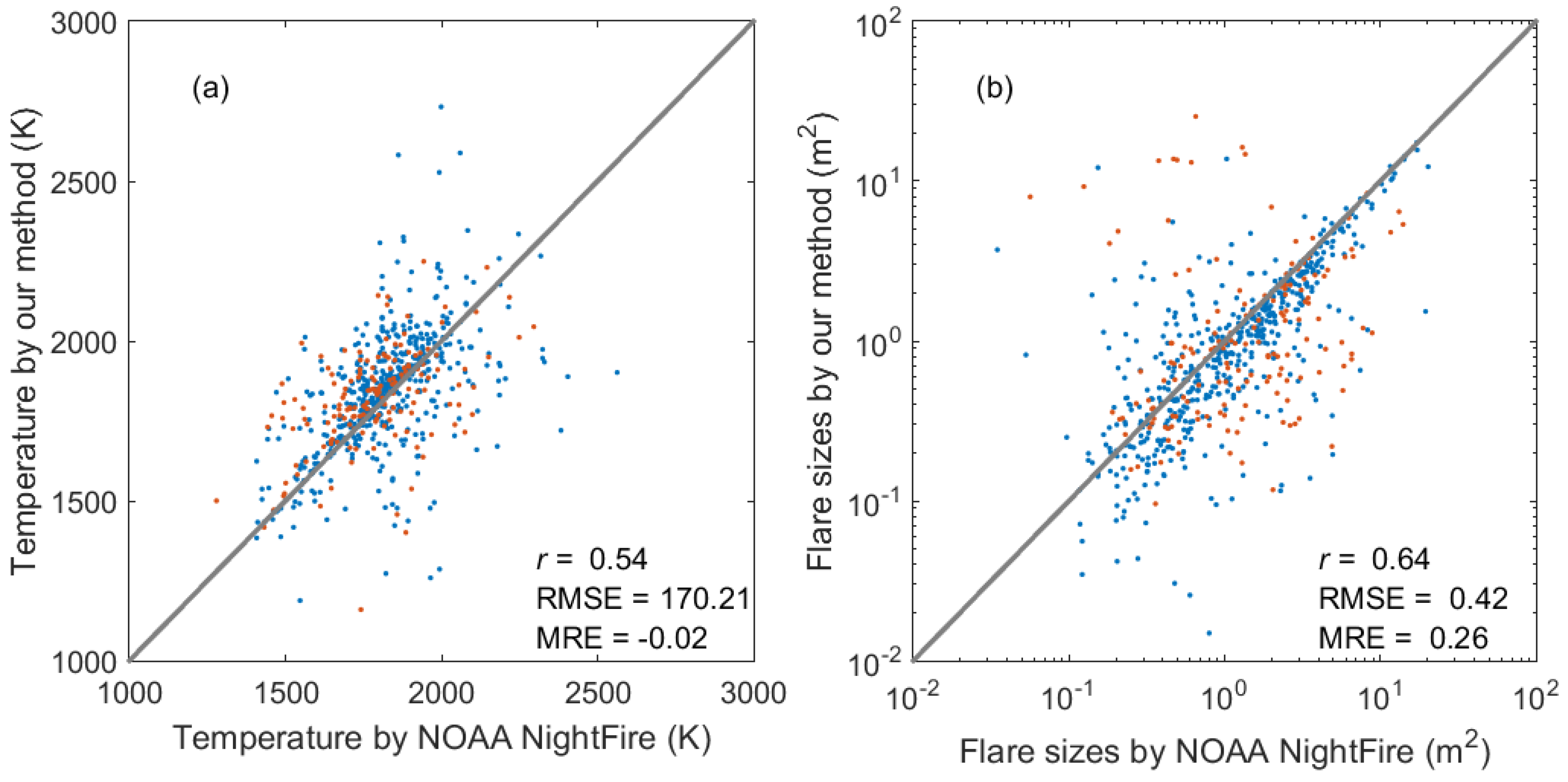
Figure 4 compares the temperatures (a) and effective areas (b) estimated for all of the flares that have been detected within 12 h by both the NOAA NightFire algorithm and our method between January 2013 and June 2014. For the NOAA data, we only used those with viewing angles <32° (i.e., in aggregation Zone 1). The scatter of the comparison is expected because of the methodological differences in detecting the flares and estimating their temperatures between the two methods. The NOAA NightFire algorithm uses the spatial contrast to identify a flare, particularly at the band M10 (
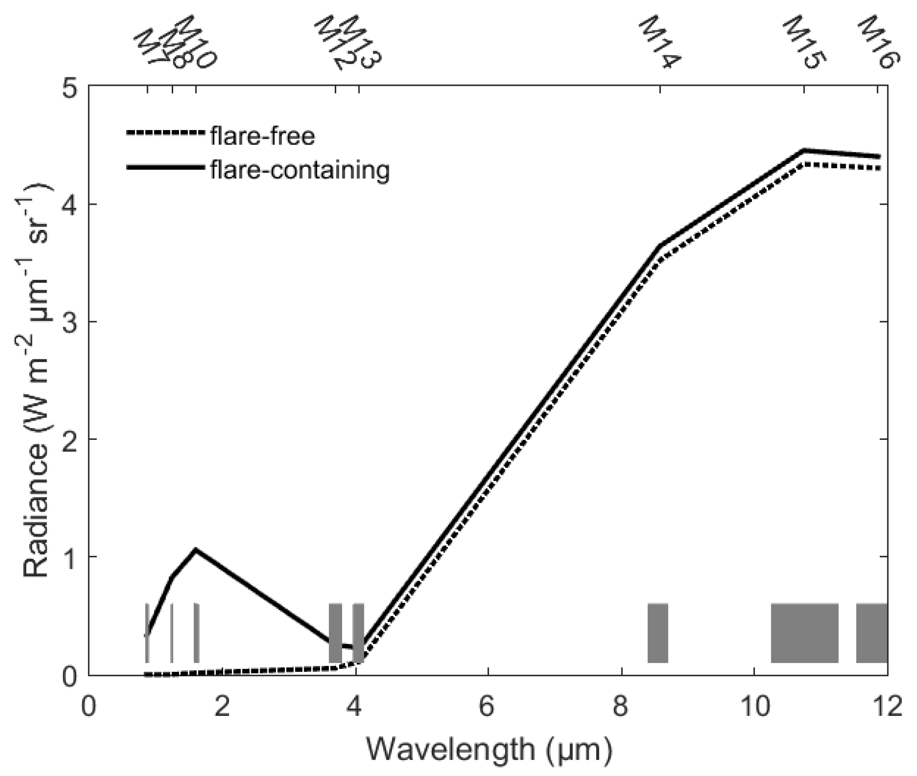
i.e., M10 for a flare is higher than the values of its neighboring pixels), whereas our method used the spectral difference to identify a flare, for which the radiance at the band M10 is greater than the value at the band M12. This detection difference arises from the fact that the NOAA NightFire algorithm is designed for the more general purpose of detecting hot sources with a wide range in temperature, while our algorithm was designed specifically for detecting flares, whose temperatures vary in a relatively tighter range of 1500–3000 K [16,17] and for which the emittance at M10 is always greater than that at M12. In addition, the NOAA NightFire algorithm uses the bands M7, M8, M10, M12 and M13 for retrieval of flare temperature [17], whereas our method used Bands M7, M8, M10, M12, M13, M14, M15 and M16 (see Figure 2). For the background, the NOAA NightFire algorithm only removes the background signal from Bands M12 and M13, whereas our method accounted for the background over all of the bands using neighboring pixels (see Equation (4)). Furthermore, atmospheric correction is performed for the NightFire data, whereas our method has assumed that the atmospheric transmittance τ = 1. Despite these differences in methodology, the two methods agree with each other reasonably well in estimating the temperatures and the areas of flares. For temperature, there is no systematic bias (the mean relative error is almost zero) and an absolute difference (as measured by root mean square error) of about 170 K; for area, the absolute difference is <0.5 m2, and the mean difference 26%. Furthermore, we did not find any significant difference in comparison between Versions 1 and 2 of the NOAA NightFire products.
Figure 4. Comparison of the temperatures (a) and effective areas (b) estimated for the flares by the NOAA NightFire algorithm and our method. Also shown are the statistical evaluation of the comparison in terms of correlation coefficient (r), root mean square error (RMSE) and mean relative error (MRE). The blue dots are for NightFire V1 data and red dots V2.
Remotesensing 07 09529 g004
However, the comparison will be worse if we include NOAA data with viewing angles >32° (i.e., in aggregation Zones 2 or 3). For example, r, RMSE and MRE would be 0.44, 202 and −0.02, respectively, for temperature comparison; and 0.55, 0.50 and 0.33, respectively, for area comparison. As discussed earlier, a flare only occupies a tiny fraction of a VIIRS pixel (<1/5000), and hence, its detection is very sensitive to contamination or deterioration of signals. The pixels located towards the edges of VIIRS imagery would have a lower signal-to-noise ratio, a larger footprint size and, hence, a smaller contribution by a flare to the signal, longer atmospheric attenuation of the signal and are subject to bowtie deletion, all of which could potentially affect the detection and characterization of flares.
The NOAA NightFire product and the results of this study that collocate with the field data within 800 m (approximately the size for one VIIRS pixel) are averaged into monthly values for comparison with the field data. Again, we only used NOAA data with viewing angles <32°. 
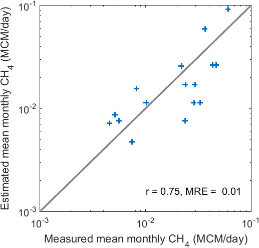
Figure 5 shows the comparison for CH4 consumption. There is a significant difference between the two versions of the NOAA NightFire estimates in CH4 rates. For Version 1, the NOAA results underestimate the field data (MRE = −0.73) with a correlation coefficient of 0.37; for Version 2, the NOAA results overestimate the field data (MRE = 7.63) and r = 0.26. On the other hand, our estimates show significant correlation with field data (r = 0.75) with an underestimation of 50%. We need to point out that our method, due to its more stringent image selection scheme, results in only 16 matches with the monthly field data, whereas there were 57 matches between the NOAA NightFire results and the monthly field data. Among the 57 matches, 37 are from the Version 1 product and 20 from Version 2. For the total energy output of methane burning (Eout in Equation (6)), we use methane’s lower heating value (LHV) of 802 (kJ/mol) [24], whereas NOAA’s NightFire algorithm uses the higher heating value (HHV) of 889 (kJ/mol), which would lead to about 10% underestimates in CH4 consumption if everything else is the same. We do not know whether and what values the NightFire algorithm uses for the other parameters (α, C and F in Equation (7)) in estimating CH4 consumption. However, it is beyond the scope of this study to investigate the methodological details of the NOAA NightFire product on flaring.
Figure 5. Comparison of methane consumed in million cubic meter per day (MCM/day) through flaring between field and remote sensing estimates. Also shown in the legend are the correlation coefficient (r) and mean relative error (MRE) between the satellite estimates and the field data. The grey line represents a 1:1 relationship.
Remotesensing 07 09529 g005
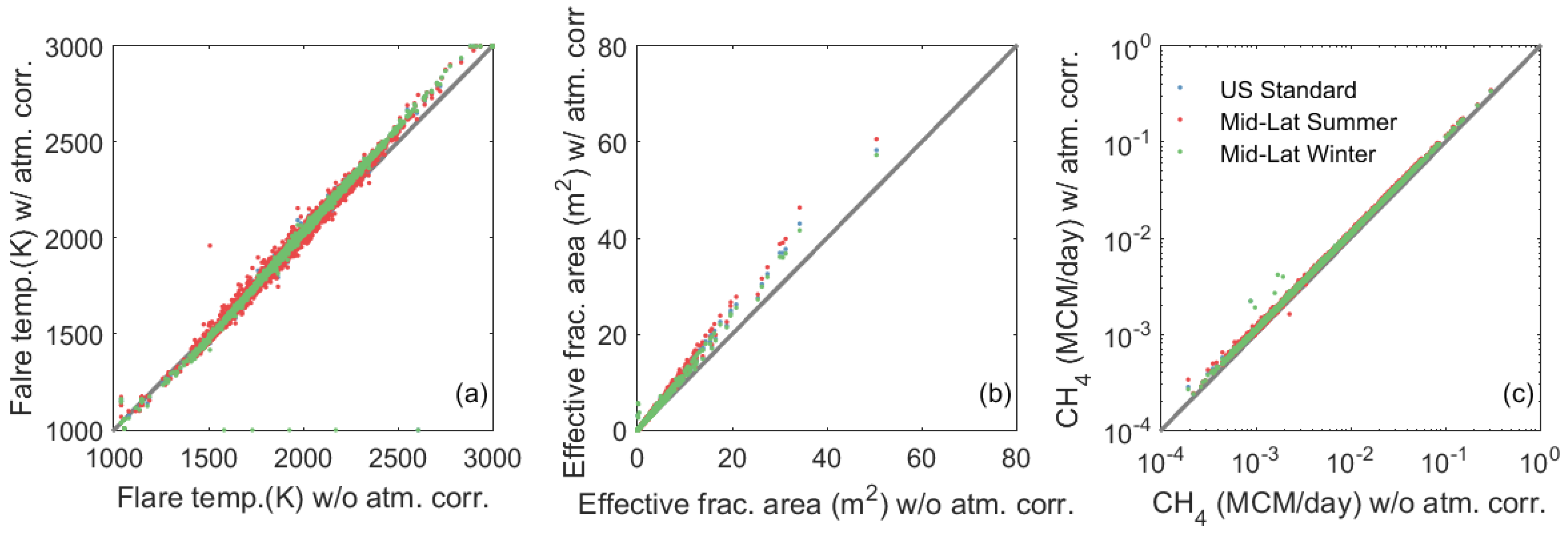
With the current setup, our results are expected to underestimate the consumption rates for two reasons: (1) the atmospheric correction is not applied; and (2) the minimum value of α has been assumed. As mentioned above, we did not apply the atmospheric correction to the VIIRS data. To evaluate its effect on the retrieval of CH4 consumption, we used the MODTRAN radiative transfer model to estimate the transmittance, i.e., τ in Equation (5) for the VIIRS bands with three different atmospheric models: mid-latitude summer atmosphere, mid-latitude winter atmosphere and 1976 U.S. standard atmosphere. The first two atmospheric models generally apply to Bakken field, and the last model has been widely used in related studies [14,17]. Elvidge et al. [17] found that non-atmospherically-corrected estimates of temperature highly correlated with, yet on average underestimate, the atmospherically-corrected results, with an underestimation ranging from 0.1% to 4% for flare temperatures of 1500–2500 K. Underestimation of a similar magnitude was also reported by Giglio and Kendall [14]. Our results (Figure 6a) are generally consistent with these earlier studies. With atmospheric correction, the effective fractional areas estimated for the flares are greater than the estimates without atmospheric correction (Figure 6b), also consistent with the results of Elvidge et al. [17]. Applying atmospheric correction, the estimates of CH4 consumption would generally be 10% greater than the estimates without atmospheric correction (Figure 6c). However, this difference cannot fully explain the underestimation of CH4 consumption, which is on average 50% lower, when compared to the field data (Figure 5).
We have assumed α = 1 in the estimation of CH4 consumption (Equation (7)), where α represents the ratio of flare area to the cross-section area of the flare that a satellite sensor sees. Its value varies with the shape of a flare, but is always greater than one. For example, if we set α = 2, our estimates would on average agree with the field data with an MRE = 1%; if we set α = 3, our estimates would on average overestimate the field data with an MRE = 51%.
Figure 6. Effect of atmospheric correction (atm. corr.) on the estimates of flaring temperature (temp.) (a), effective fractional (frac.) area (b) and CH4 consumption (c). The grey line represents a 1:1 relationship. Three different atmospheric models available in MODTRAN have been tested: mid-latitude summer, mid-latitude winter and 1976 U.S. standard.
Remotesensing 07 09529 g006
The ratio of surface to cross-section areas α, combustion efficient C and F-factor F cannot be derived from remote sensing, and therefore, their values have to be assumed. Furthermore, all of these three parameters decrease with wind speeds. For α, the stronger the wind, the more surface is exposed to a satellite sensor, and hence, its value becomes lower. On the other hand, the higher the wind, the greater the surface area (fe) of a flare would expose to a sensor from above. Therefore, the combined effect of wind on the value of α × fe is reduced compared to individual effects. For the F-factor (F), both observation and the model show that its value decreases with wind speeds, and the value of F for methane varies between 10% and 30% [24]. The combustion efficiency (C) is relatively insensitive to wind speeds, even though its value can be lower under high wind conditions [26]. Since the estimate of gas flaring is proportional to α f e C F   (Equation (7)), in which three parameters (α, C and F) decrease and 
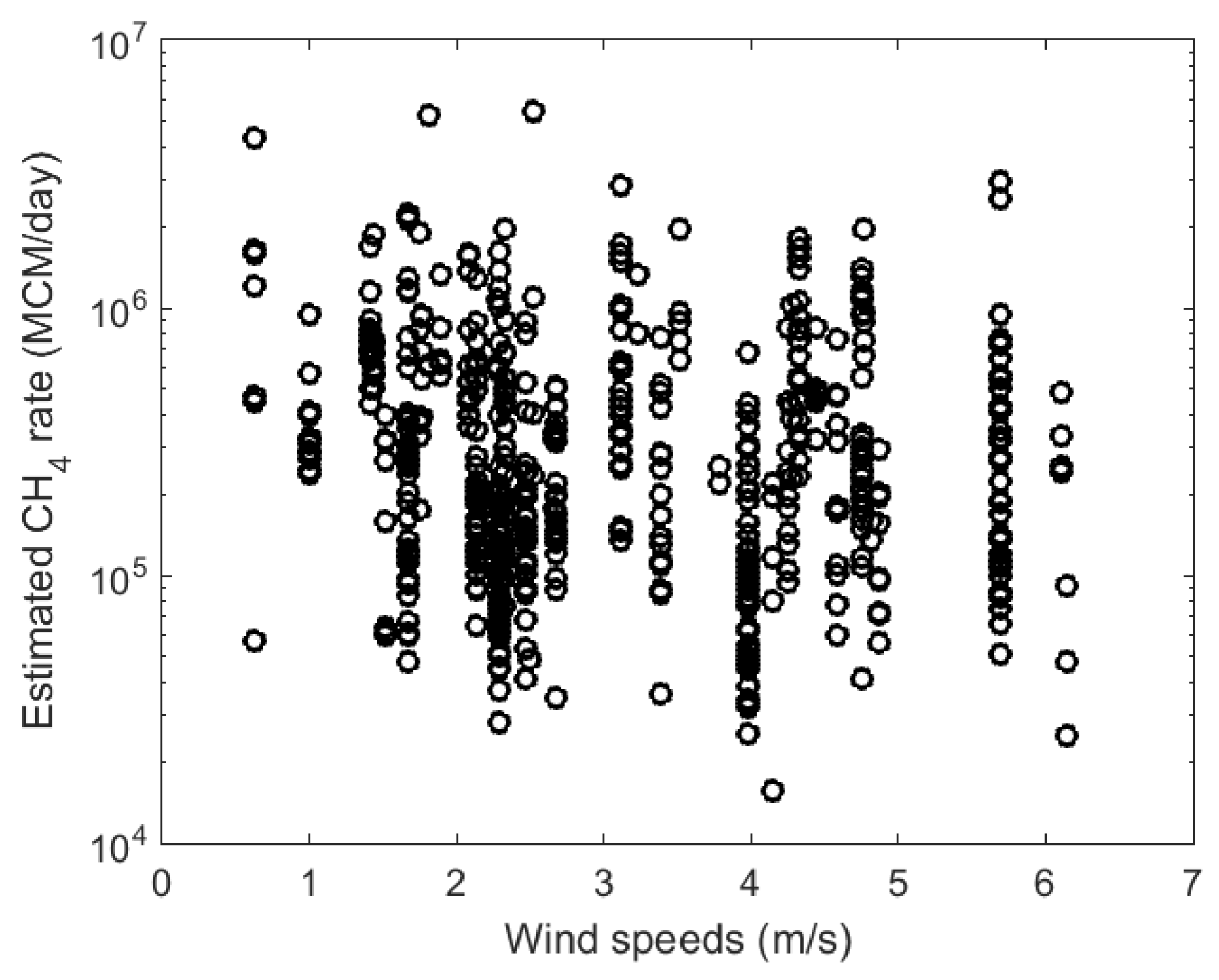
fe increases with wind speed, at least some the wind dependence is cancelled out. The exact impact of wind conditions on estimating gas consumption and emission needs to be investigated further. From our results, we did not find any significant co-variation between the estimates of CH4 consumption and wind conditions (r = −0.1) in this study (Figure 7).
Figure 7. The estimated daily CH4 consumption vs. the wind speeds.
Remotesensing 07 09529 g007

4. Conclusions

In this study, a model was developed to estimate methane consumption of gas flaring using VIIRS nighttime data. Our estimates in methane consumption compared reasonably well with limited field data, whereas the NOAA NightFire estimates showed underestimation with Version 1 and overestimation with Version 2 (Figure 5). There are significant differences in methodology between the NOAA NightFire algorithm and our method. First, we applied a more stringent data screening filter, retaining only those images that are cloud free and in the middle portion of a scene. Because flares are an extremely small object within a pixel of the VIIRS sensor, any contamination due to cloud or deterioration of the flare signal recorded at a large viewing angle would directly affect the detection of flares. Additionally, the comparison on temperature and effective area of flares between the NightFire and our method did improve when the NightFire data with viewing angles >32° were excluded. Second, we adopted Giglio and Kendall’s [14] method using neighboring pixel(s) as the background and the spectral radiance at eight bands (M7, M8, M10, M12, M13, M14, M15 and M16) to derive the thermal temperature and fractional area of a flare (Equation (5)). Third, the lower heating value for methane combustion was used for calculations of thermal emissions and emissivity, which is more appropriate than the higher heating value that the NOAA NightFire algorithm uses. Finally, efficiency factors were accounted for to provide greater accuracy in calculating completeness in combustion and conversion of total reaction energy into radiant energy that can be sensed by a satellite sensor (Equation (7)).
Remaining uncertainties include determining the exact value for α, relating the area of a flare to its cross-section area that a satellite sensor sees from above. This value depends on the shape of the flare, but might vary in a tight range between one and three, within which our results agreed with the field data within ±50%. Further improvement of the method employed in this work can be achieved by using atmospherically-corrected VIIRS nighttime data; however, the improvement in using atmospherically corrected data is limited because the major uncertainty remains estimating the form factor of the flares.
We have validated the results using the field data collected in Bakken field. However, we believe the method is applicable to detecting and quantifying gas flaring in general, with the only assumption being that there exist neighboring pixel(s) with similar land and atmospheric conditions. Even though it is not evaluated in this study, it is straightforward to estimate the emission of CO2 using Equation (8) through gas flaring, which is one of our planned future works in continuing this study.

Acknowledgments

The study results from collaborative research between the Department of Earth System Science and Policy and the Energy & Environmental Research Center funded by the University of North Dakota’s Collaborative Seed Grants.

Author Contributions

XZ, CZ and CW designed the study. CZ and CW provided field data. B. Scheving and B. Shoghli analyzed the data. XZ, B. Scheving and B. Shoghli developed algorithm. All contributed to the writing of the manuscript.

Conflicts of Interest

The authors declare no conflict of interest.

References

  1. Blasing, T.J.; Hand, K. Monthly carbon emissions from natural-gas flaring and cement manufacture in the United States. Tellus B 2007, 59, 15–21. [Google Scholar] [CrossRef]
  2. Ford, M.; Davis, N. Nonmarketed natural gas in North Dakota still rising due to higher total production. Available online: http://www.eia.gov/todayinenergy/detail.cfm?id=15511 (accessed on 3 July 2015).
  3. Budzik, P.; Ford, M. North Dakota aims to reduce natural gas flaring. Available online: http://www.eia.gov/todayinenergy/detail.cfm?id=18451 (accessed on 3 July 2015).
  4. Ichoku, C.; Kahn, R.; Chin, M. Satellite contributions to the quantitative characterization of biomass burning for climate modeling. Atmos. Res. 2012, 111, 1–28. [Google Scholar] [CrossRef]
  5. Dozier, J. A method for satellite identification of surface temperature fields of subpixel resolution. Remote Sens. Environ. 1981, 11, 221–229. [Google Scholar] [CrossRef]
  6. Prins, E.M.; Menzel, W.P. Geostationary satellite detection of bio mass burning in South America. Int. J. Remote Sens. 1992, 13, 2783–2799. [Google Scholar] [CrossRef]
  7. Prins, E.M.; Menzel, W.P. Trends in South American biomass burning detected with the GOES visible infrared spin scan radiometer atmospheric sounder from 1983 to 1991. J. Geophys. Res.: Atmos. 1994, 99, 16719–16735. [Google Scholar] [CrossRef]
  8. Matson, M.; Dozier, J. Identification of subresolution high temperature sources using a thermal IR sensor. Photogramm. Eng. Remote Sens. 1981, 47, 1311–1318. [Google Scholar]
  9. Matson, M.; Stephens, G.; Robinson, J. Fire detection using data from the NOAA-N satellites. Int. J. Remote Sens. 1987, 8, 961–970. [Google Scholar] [CrossRef]
  10. Giglio, L.; Kendall, J.D.; Tucker, C.J. Remote sensing of fires with the TRMM VIRS. Int. J. Remote Sens. 2000, 21, 203–207. [Google Scholar] [CrossRef]
  11. Giglio, L.; Csiszar, I.; Justice, C.O. Global distribution and seasonality of active fires as observed with the Terra and Aqua Moderate Resolution Imaging Spectroradiometer (MODIS) sensors. J. Geophys. Res.: Biogeosci. 2006, 111, G02016. [Google Scholar] [CrossRef]
  12. Justice, C.O.; Giglio, L.; Korontzi, S.; Owens, J.; Morisette, J.T.; Roy, D.; Descloitres, J.; Alleaume, S.; Petitcolin, F.; Kaufman, Y. The MODIS fire products. Remote Sens. Environ. 2002, 83, 244–262. [Google Scholar] [CrossRef]
  13. Csiszar, I.; Schroeder, W.; Giglio, L.; Ellicott, E.; Vadrevu, K.P.; Justice, C.O.; Wind, B. Active fires from the Suomi NPP Visible Infrared Imaging Radiometer Suite: Product status and first evaluation results. J. Geophys. Res.: Atmos. 2014, 119, 803–816. [Google Scholar] [CrossRef]
  14. Giglio, L.; Kendall, J.D. Application of the Dozier retrieval to wildfire characterization: a sensitivity analysis. Remote Sens. Environ. 2001, 77, 34–49. [Google Scholar] [CrossRef]
  15. Leahey, D.M.; Davies, M.J.E. Observations of plume rise from sour gas flares. Atmos. Environ. (1967) 1984, 18, 917–922. [Google Scholar] [CrossRef]
  16. Kaufman, Y.J.; Justice, C.O.; Flynn, L.P.; Kendall, J.D.; Prins, E.M.; Giglio, L.; Ward, D.E.; Menzel, W.P.; Setzer, A.W. Potential global fire monitoring from EOS-MODIS. J. Geophys. Res.: Atmos. 1998, 103, 32215–32238. [Google Scholar] [CrossRef]
  17. Elvidge, C.; Zhizhin, M.; Hsu, F.-C.; Baugh, K. VIIRS NightFire: Satellite pyrometry at night. Remote Sens. 2013, 5, 4423–4449. [Google Scholar] [CrossRef]
  18. Elvidge, C.; Ziskin, D.; Baugh, K.; Tuttle, B.; Ghosh, T.; Pack, D.; Erwin, E.; Zhizhin, M. A fifteen year record of global natural gas flaring derived from satellite data. Energies 2009, 2, 595–622. [Google Scholar] [CrossRef]
  19. Cao, C.; Xiong, J.; Blonski, S.; Liu, Q.; Uprety, S.; Shao, X.; Bai, Y.; Weng, F. Suomi NPP VIIRS sensor data record verification, validation, and long-term performance monitoring. J. Geophys. Res.: Atmos. 2013, 118, 11,664–11,678. [Google Scholar] [CrossRef]
  20. Pollastro, R.M.; Roberts, L.N.R.; Cook, T.A. Geologic assessment of technically recoverable oil in the devonian and mississippian bakken formation. In Assessment of Undiscovered Oil and Gas Resources of the Williston Basin Province of North Dakota, Montana, and South Dakota, 2010 (ver. 1.1, November 2013): U.S. Geological Survey Digital Data Series 69-W; U.S. Geological Survey Williston Basin Province Assessment Team, Ed.; U.S. Geological Survey: Reston, VA, USA, 2013; p. 38. [Google Scholar]
  21. Changyong, C.; de Luccia, F.J.; Xiaoxiong, X.; Wolfe, R.; Fuzhong, W. Early on-orbit performance of the Visible Infrared Imaging Radiometer Suite Onboard the Suomi National Polar-Orbiting Partnership (S-NPP) Satellite. IEEE Trans. Geosci. Remote Sens. 2014, 52, 1142–1156. [Google Scholar]
  22. Jin, S.; Yang, L.; Danielson, P.; Homer, C.; Fry, J.; Xian, G. A comprehensive change detection method for updating the National Land Cover Database to circa 2011. Remote Sens. Environ. 2013, 132, 159–175. [Google Scholar] [CrossRef]
  23. Jin, M.; Liang, S. An improved land surface emissivity parameter for land surface models using global remote sensing observations. J. Clim. 2006, 19, 2867–2881. [Google Scholar] [CrossRef]
  24. Guigard, S.E.; Kindzierski, W.B.; Harper, N. Heat radiation from flares. Reports prepared for Science and Technology Branch; Alberta Environment: Edmonton, AB, Canada, 2000; p. 90.
  25. Leahey, D.M.; Preston, K.; Strosher, M. Theoretical and observational assessments of flare efficiencies. J. Air Waste Manage. Assoc. 2001, 51, 1610–1616. [Google Scholar] [CrossRef]
  26. Cain, J.; Seebold, J.; Young, L. Overview of Flaring Efficiency Studies; ChevronTexaco Energy Research and Technology Company: San Ramon, CA, USA, 2002; p. 12. [Google Scholar]

