1. Introduction
The degree to which an Earth-observing remote sensing platform is able to assign accurate geographic positions to the surface features being imaged is referred to as its geolocation accuracy. A spaceborne Synthetic Aperture Radar (SAR) sensor with high geolocation accuracy greatly simplifies the task of combining multiple images with one another, not only for inter-comparisons, but also to dramatically speed up applications, such as near-real-time disaster mapping. Accurate geolocation, dependent on radar system timing, permits multiple image products to be quickly combined, e.g., expediting SAR interferometry (InSAR) coregistration or layered with other data sources, such as digital elevation models (DEMs), cadastral maps, vegetation maps, forest maps, hydrological maps,
etc. A good example of this type of layering is described in [
1], whereby long time series can be quickly and automatically radiometrically terrain-corrected using a Digital Terrain Model (DTM), useful for, e.g., wet-snow monitoring. Sentinel-1A (S1A) provides a continual supply of all-weather, day-or-night imagery of the Earth’s surface which can be used for time series analyses, or combined with data from other platforms or sensors. For these goals to be feasible, S1A products [
2] are required to provide high and consistent geolocation accuracy, as specified in Tables 7-1 through 7-10 of [
2].
During the S1A in-orbit commissioning phase, the SAR team at the Remote Sensing Laboratories, University of Zurich (UZH), Switzerland, performed mission performance monitoring for the S1A product geometric calibration and validation. Preliminary geolocation estimates were provided in [
3]. S1A reached its designated reference orbit on 7 August 2014, providing the stable SAR imaging geometry required for performing highly accurate geolocation measurements. Since then, many more SAR acquisitions have been collected and analyzed.
The Sentinel-1 SAR instrument operates at 5.405 GHz (C-band, corresponding to a radar wavelength of about 5.6 cm) and supports four exclusive imaging modes providing different resolution and coverage: Interferometric Wide Swath (IW), Extra Wide Swath (EW), StripMap (SM), and Wave (WV) [
4].
Table 1 provides the product resolutions and sample spacings for the modes relevant to geometric calibration/validation. The IW mode is the main mode of operations for the Sentinel-1 mission, enabling the systematic monitoring of large land and coastal areas at a ground resolution of 5 m × 20 m. The SM mode, due to its fine slant range and azimuth resolutions of between ~2–5 m, is subject to more stringent requirements for geolocation accuracy. For this reason, this paper focuses on the calibration and validation of the geolocation accuracy for S1A SM Single Look Complex (SLC) and Ground Range Detected Fine-resolution (GRDF) image products. As described in [
5], the Sentinel-1 SM mode is comprised of six beams,
i.e., SM1–SM6, covering an incident angle range of 20°–43°. While SM acquisitions are not as commonly available as IW or EW products, the use of SM products for geometric calibration naturally also improves the expected accuracy of the wide swath products, acquired using the same beams.
For the validation of the S1A SM product geolocation accuracy, it is important to understand and exclude the largest known sources of error. Unavoidable technical challenges for such systems are orbital stability and positional accuracy; both set limits on the achievable localization accuracy of imaged ground targets.
In addition to orbit- and sensor-specific technical challenges, achieving the highest-possible accuracy from SAR image products requires correcting for at least two perturbing factors [
6,
7,
8]:
(a) The effect of the troposphere and ionosphere on the signal travel time, called atmospheric path delay (PD), can cause errors typically on the order of several meters if neglected. The tropospheric component is the largest, caused by hydrostatic (air pressure), wet (water vapor), and liquid (water droplet) variations along the signal travel path.
(b) The solid Earth tide (SET), a periodic (mainly vertical) oscillation of the Earth’s crust on the order of 1–2 decimeters, caused primarily by the moon and sun.
When using surveyed reference targets on the ground, an additional correction needs to be made. In this study, a set of four and two corner reflectors (CRs), deployed consecutively at two test sites, were surveyed using Differential GPS (DGPS). Because of the drift between local and global geodetic reference frames resulting from plate tectonics, the coordinates provided by the GPS alone are usually shifted relative to the International Terrestrial Reference Frame (ITRF) employed to describe the spacecraft positions. This effect can be corrected by transforming the GPS position into the global frame through the use of a plate tectonic drift model.
Table 1.
Level 1 Product Family Summary; adapted from Table 5-1 in [
2].
Table 1.
Level 1 Product Family Summary; adapted from Table 5-1 in [2].
| Acq. Mode | Product Type | Resolution Class | Resolution 1,2 [Rg × Az] 3 [m] | Pixel Spacing 2 [Rg × Az] [m] | No. Looks [Rg × Az] | ENL 4 |
|---|
| SM | SLC | | 1.7 × 4.3 to 3.6 × 4.9 | 1.5 × 3.6 to 3.1 × 4.1 | 1 × 1 | 1 |
| GRD | FR | 9 × 9 | 3.5 × 3.5 | 2 × 2 | 3.7 |
| HR | 23 × 23 | 10 × 10 | 6 × 6 | 29.7 |
| MR | 84 × 84 | 40 × 40 | 22 × 22 | 398.4 |
| IW | SLC | | 2.7 × 22 to 3.5 × 22 | 2.3 × 14.1 | 1 | 1 |
| GRD | HR | 20 × 22 | 10 × 10 | 5 × 1 | 4.4 |
| MR | 88 × 87 | 40 × 40 | 22 × 5 | 81.8 |
| EW | SLC | | 7.9 × 43 to 15 × 43 | 5.9 × 19.9 | 1 × 1 | 1 |
| GRD | HR | 50 × 50 | 25 × 25 | 3 × 1 | 2.7 |
| MR | 93 × 87 | 40 × 40 | 6 × 2 | 10.7 |
We refer to perturbations caused by SET and plate tectonics together as “solid-Earth perturbations”, since they affect the position of targets situated on solid ground. Even smaller effects also exist: e.g., Earth deformation by ocean tide loading. As the oceans are periodically redistributed by the relative positions of the Sun-Moon-Earth system, the changing weight distribution of the water mass on the ocean bed causes the Earth to deform. These vertical fluctuations usually do not exceed several centimeters for inland sites [
9] and are neglected in this study.
2. Experiment Design
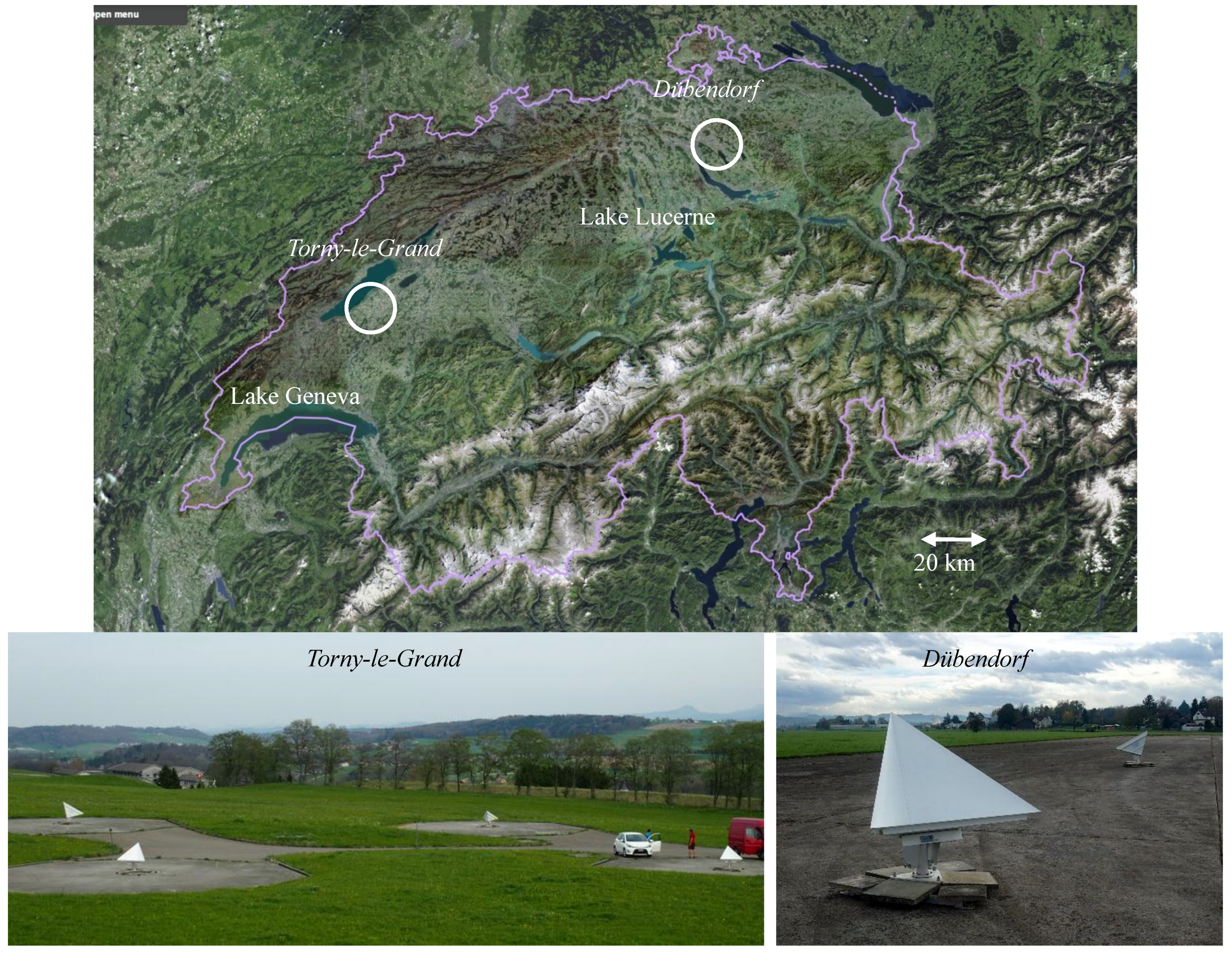
Two test sites in Switzerland were selected for the placement of the trihedral CRs that served as geometric reference targets. They are indicated at the top of
Figure 1. The CR sizes ranged from 90 cm to 120 cm, large enough to be visible as bright “point targets” in the SM mode images. The first site was in the west of Switzerland near the village of
Torny-Le-Grand, which had been used successfully in the past for a similar long-term experiment [
7] devoted to the analysis of TerraSAR-X data. Four trihedral CRs were placed at the site, with two facing the S1A sensor in its ascending orbit and two facing its descending orbit (bottom left of
Figure 1). A permanent GPS reference station of the Automated Global Navigation Satellite System Network of Switzerland (AGNES), located < 5 km from the site near the town of
Payerne, was used for the differential positioning. Trimble R7 GPS receivers were used to measure their locations with accuracies better than 1 cm (confirmed by Chapter 8 in [
10]). The pair-wise arrangement of the CRs not only created redundancy (in case of problems with one reflector) but also served to help validate the accuracy of their positions, as identical geolocation results should in principle be obtained for both CRs of a given pair. For each reflector, a fixed reference point on the concrete surface was surveyed; the reflector was mounted above it with the correct orientation and elevation, and the offset to its phase center (corner) was measured.
Figure 1.
University of Zurich (Switzerland) corner reflector test sites Torny-le-Grand and Dübendorf. Four reflectors (two per orbital direction) were located at Torny-le-Grand from April to October 2014, then two (one per orbital direction) at Dübendorf from October 2014 to January 2015.
Figure 1.
University of Zurich (Switzerland) corner reflector test sites Torny-le-Grand and Dübendorf. Four reflectors (two per orbital direction) were located at Torny-le-Grand from April to October 2014, then two (one per orbital direction) at Dübendorf from October 2014 to January 2015.
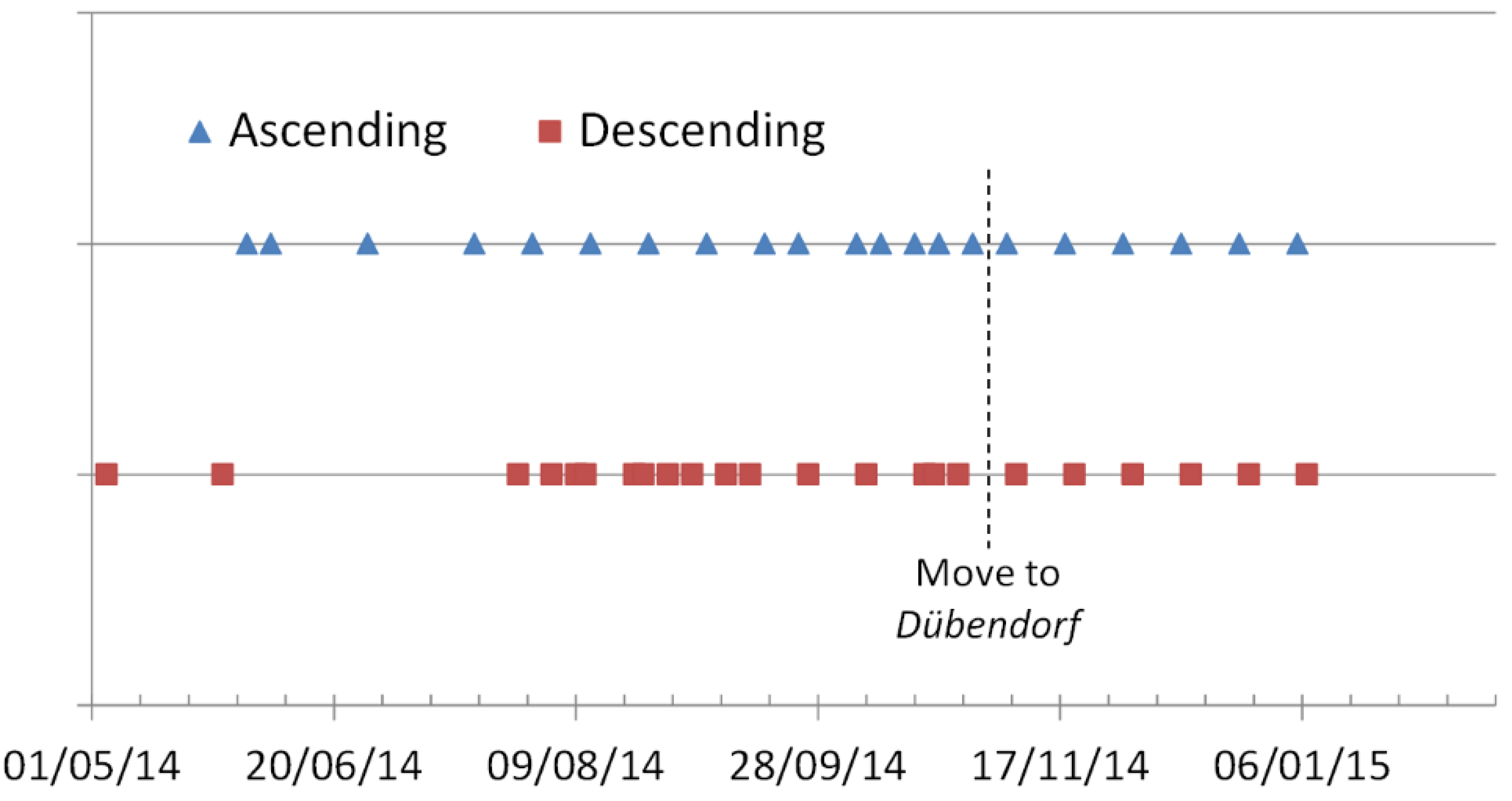
S1A acquisitions were obtained over Torny-le-Grand from 4 May to 30 October 2014, although the few very early products (until the beginning of June 2014) were deemed too unreliable for geolocation estimation, possibly because of orbital uncertainties. The site was no longer available to UZH after October 2014, so a new site (Dübendorf) was used for the remainder of the calibration phase.
On 4 November 2014, two CRs (with 1 m and 1.2 m side lengths) were placed at the
Dübendorf test site (indicated at the top of
Figure 1) and their positions surveyed using DGPS, this time using an AGNES reference station in nearby Zurich (station code
ETH2).
Table 2 lists the approximate test site positions in WGS84 geographic coordinates.
Table 2.
Approximate test site positions in WGS84 geographic coordinates.
Table 2.
Approximate test site positions in WGS84 geographic coordinates.
| Test Site | Longitude [°] | Latitude [°] | Height above Ellipsoid [m] |
|---|
| Torny-le-Grand | 6.956008 | 46.770323 | 779.0 |
| Dübendorf | 8.647244 | 47.397544 | 487.2 |
Figure 2.
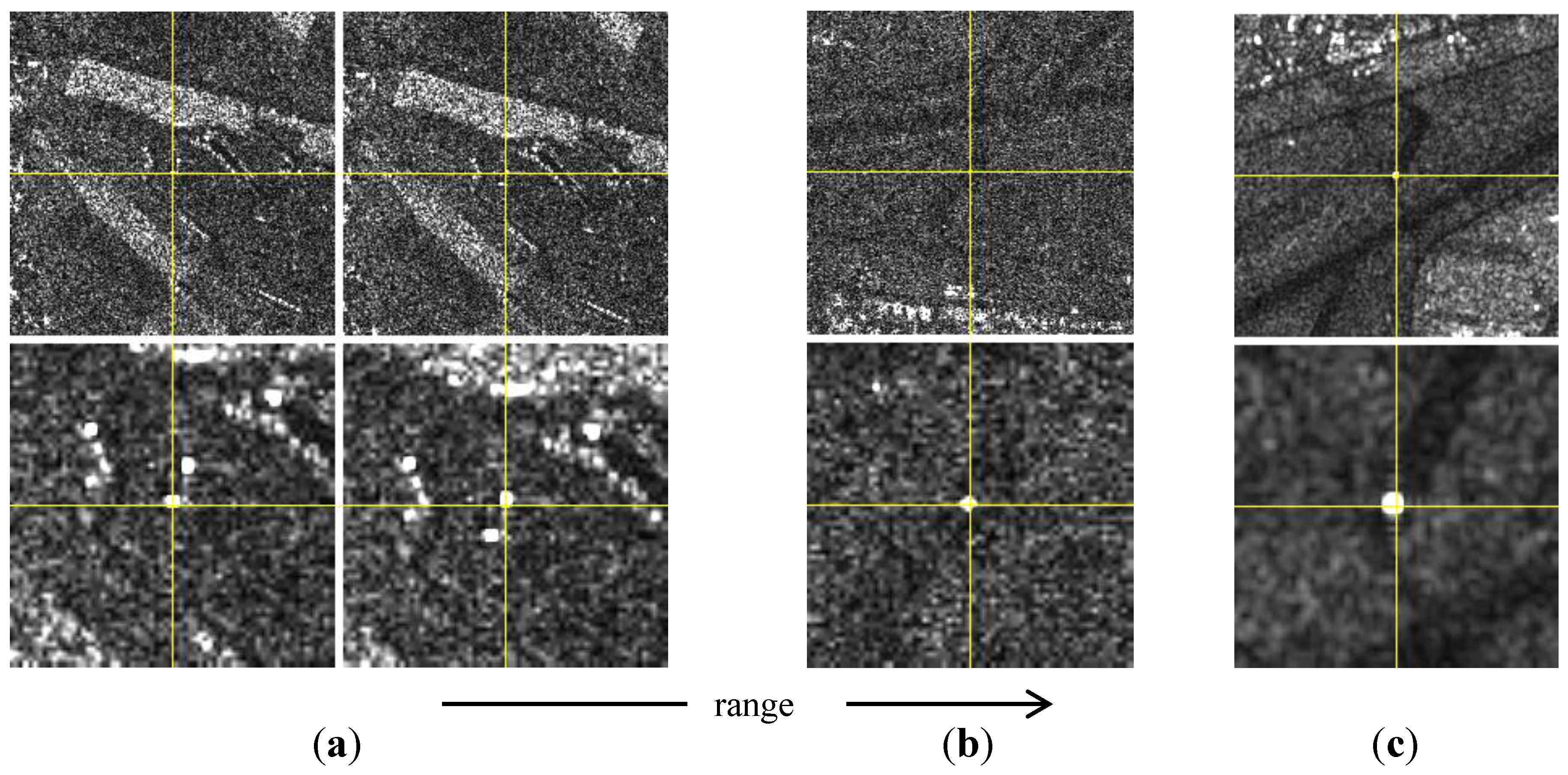
Corner reflectors as seen in S1A StripMap products, with predicted positions indicated by the yellow crosshairs in each case and a higher zoom level at the bottom; (a) SLC over Torny-le-Grand, north-west reflector (left) and south-west reflector (right), product S1A_S6_SLC__1SDV_20140627T172926_20140627T172949_001239_001318_53C9.SAFE; (b) SLC over Dübendorf, product S1A_S3_SLC__1SDV_20150107T054240_20150107T054303_004061_004E73_ACA0.SAFE; (c) GRDF over Dübendorf, product S1A_S2_GRDF_1SDV_20141118T170652_20141118T170721_003339_003DF1_99A0.SAFE. (Copernicus Sentinel data 2014–2015).
Figure 2.
Corner reflectors as seen in S1A StripMap products, with predicted positions indicated by the yellow crosshairs in each case and a higher zoom level at the bottom; (a) SLC over Torny-le-Grand, north-west reflector (left) and south-west reflector (right), product S1A_S6_SLC__1SDV_20140627T172926_20140627T172949_001239_001318_53C9.SAFE; (b) SLC over Dübendorf, product S1A_S3_SLC__1SDV_20150107T054240_20150107T054303_004061_004E73_ACA0.SAFE; (c) GRDF over Dübendorf, product S1A_S2_GRDF_1SDV_20141118T170652_20141118T170721_003339_003DF1_99A0.SAFE. (Copernicus Sentinel data 2014–2015).
Extracts from three SM products are shown in
Figure 2, with yellow crosshairs indicating the automatically predicted CR image locations, and two zoomed imagettes centered on those CR positions. In
Figure 2a, two extracts from SM Single Look Complex (SLC) products are centered on the ascending-orbit reflectors at
Torny-le-Grand.
Figure 2b is from a similar SM SLC product, but centered on a product acquired over the
Dübendorf site. In
Figure 2c one of the
Dübendorf reflectors is visible in an extract from an SM ground range fine-resolution (GRDF) product. The GRDF products have a coarser sample spacing (4 m azimuth and ground range) than SLC products generated from the same acquisition.
A total of 44 SM acquisitions were obtained over both test sites during the observation period, from 4 May 2014 to 7 January 2015. The first three of these acquisitions (before early June 2014) had to be eliminated due to problems possibly caused by the early orbital maneuvers required for the satellite to reach its reference orbit. For all of these acquisitions, both the SLC and GRDF products were obtained. Only the SLC products, which maintain the full sensor resolution, were used for estimation of the processor-inherent range and azimuth biases. GRDF products were tested for validation purposes (as opposed to sensor calibration), in particular the quality of the slant to ground range projection. The acquisition timeline is shown in
Figure 3.
Figure 3.
S1A StripMap acquisition time series over Torny-le-Grand and Dübendorf.
Figure 3.
S1A StripMap acquisition time series over Torny-le-Grand and Dübendorf.
4. Azimuth “Bistatic Residual” Correction
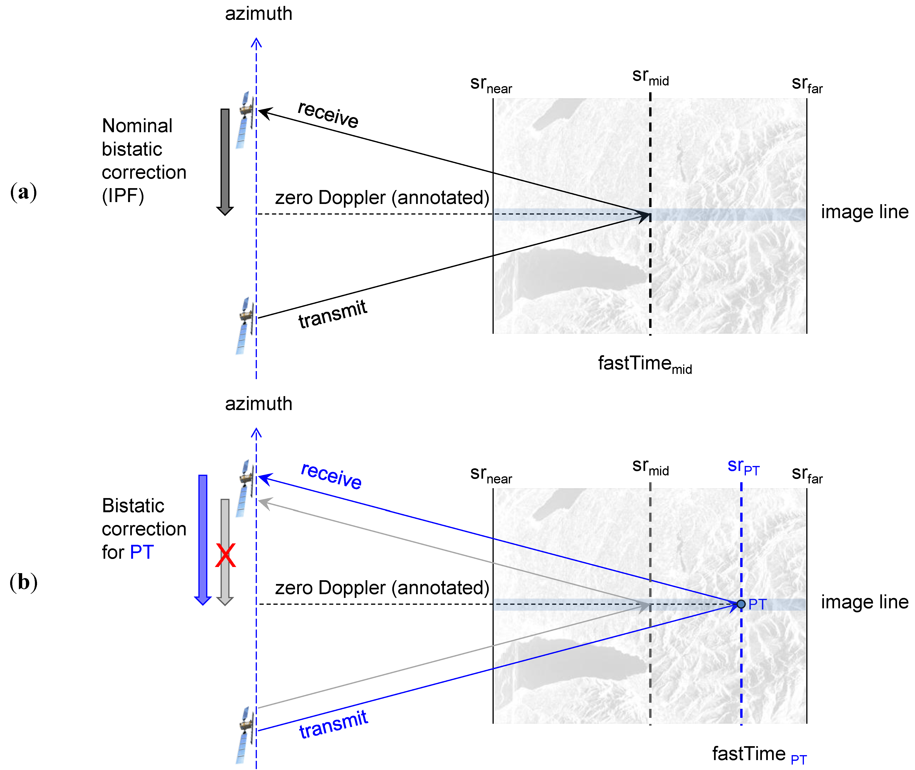
During the S1A in-orbit commissioning phase, an unexpectedly high azimuth geolocation error was discovered. Subsequent investigation shed light on the issue and led to the implementation of another necessary timing correction, this time related to the S1A operational SAR Instrument Processing Facility (IPF) itself. As illustrated in
Figure 5a for SM mode, the satellite moves a certain distance along its orbit during the time between pulse transmission and echo reception. This is referred to as the
bistatic effect or
start-stop approximation, and it has been understood for many years [
15]. For S1A, this distance is typically ~43 m at mid-scene, given e.g., a spacecraft velocity of 7592 m/s and an echo travel time (“fast time”) at mid-scene of ~5.7 × 10
−3 s (beam S4 product). Usually, a SAR system records the time when the radar echo is received, providing this in the product annotations. While this method provides a good first approximation of the azimuth times corresponding to the image lines, they are nonetheless consistently too “late”. The S1 IPF improves this method by shifting the time stamps to the moment when the side-looking sensor was actually aimed at the imaged line, as indicated in
Figure 5a. In this way, the azimuth time stamps correspond to the time when the
mid-range samples were imaged, which is a better approximation for the image line as a whole. The correction performed is thus a perfect correction at mid-range but contains an inherent error residual proportional to the slant range offset from this point. The timing correction is indicated by the gray arrow in
Figure 5a.
Critically, the magnitude of the correction applied by the S1 IPF is made under the mid-range assumption,
i.e., for a spacecraft travel time corresponding to the mid-range echo travel time, as this is the optimal choice for the image as a whole. However, the correction is insufficient when high accuracy is required for a specific target within the scene, as illustrated in
Figure 5b. Here, point target PT is imaged at the same zero Doppler time as in
Figure 5a, but the increased echo travel time relative to mid-range implies that a larger bistatic timing shift is needed relative to the echo receive moment. The bistatic shift required for PT is shown as a blue arrow in
Figure 5b. We call the
difference between the arrow lengths in
Figure 5b the
bistatic residual error. It can be as large as ~0.7 m (for a target near the SM beam S6 edge). The residual error can be expressed in seconds or meters, as given in Equations (1) and (2):
In the above equations, the fast time (echo travel time) for a given range sample at the point target PT, is calculated as follows:
Here, sr
near is the fast time at the near-range edge. It is obtained from the product annotations (auxiliary file XML file, parameter
slantRangeTime in the section product:imageAnnotation:imageInformation). rgSampleNr is the range sample number, where the first sample is numbered 0. The range sampling rate (rgSampleRate) is derived from the S1A product parameter
rangeSamplingRate in the annotation XML file under product:generalAnnotation:productInformation [
16].
The azimuth timing correction in Equation (1) is integrated into the geolocation processor as a small shift in the predicted time for a given CR.
Figure 5.
Calculation of the bistatic residual for a point target in an S1A StripMap product (a) nominal mid-range bistatic correction applied for a StripMap product by the S1 IPF as of v2.43; (b) bistatic correction needed for a point target PT at slant range srPT.
Figure 5.
Calculation of the bistatic residual for a point target in an S1A StripMap product (a) nominal mid-range bistatic correction applied for a StripMap product by the S1 IPF as of v2.43; (b) bistatic correction needed for a point target PT at slant range srPT.
5. Orbital State Vectors (OSVs)
To meet a high standard, geolocation requires not only accurate knowledge of the imaging system and Earth environment, but commensurately accurate knowledge of the Orbital State Vectors (OSVs) as well (i.e., the platform positions). Four sources for the OSVs were available: GNSS internally annotated in the source packets, predicted (S1A_OPER_MPL_ORBPRE files), near-real-time restituted (S1A_OPER_AUX_RESORB files), and precise (S1A_OPER_AUX_POEORB files). Predicted OSVs are generated separately about once a day, so their accuracy depends mainly on the interval between the file generation and the acquisition times. The precise OSVs are only currently available with a latency of three weeks, so many applications employ the restituted OSVs, which were found to be nearly as accurate.
The case of the internal OSVs is complicated. Although the GNSS state vectors injected into the source packets are inherently accurate, they are provided within the boundaries of the acquisition segment. In order to perform proper interpolation, the EO_CFI (used also by the IPF) requires ~6 state vectors before and after the product. This requirement is even more stringent in the case of products generated from one of the TOPS modes (Terrain Observation with Progressive Scan products, i.e., IW and EW), where the focused burst is extended, requiring more OSVs than are available. Simple extrapolation methods were tested but none were sufficiently robust. Consequently, given that GNSS OSV interpolation was always possible, the IPF employed the EO_CFI library in propagation mode based on a single ascending node crossing (ANX) OSV. This method is inherently less accurate; its quality quickly decreases with distance from the ANX point. Our results presented in the coming sections also confirmed that if restituted or even precise OSV files were annotated, then the geolocation quality was nearly equivalent to using the corresponding external files, as long as the orbit interpolation was sufficiently reliable. Since these initial tests, a more robust approach for using the GNSS OSVs has been implemented in the S1 IPF and is currently undergoing testing, with initial ALE estimates within the expected limits.
For the best geolocation accuracy, it is recommended that precise orbit files be used, (AUX_POEORB auxiliary files). If near-real-time is required, then the restituted AUX_RESORB orbit files were demonstrated to be nearly as accurate. The structure of these auxiliary files is described in [
17]. These were our initial source of orbital state vectors, interpolated using ESA’s EO_CFI library [
18]. A comparison of the various state vector source qualities is shown in the latter part of
Section 7 below.
7. Results and Discussion
Using the methods described in the previous sections, the ALE was estimated for all SM products acquired over the Swiss test sites after 4 June 2014 (41 acquisitions, each processed to SLC and GRDF products). Since the Torny-le-Grand products had two CRs visible in each image, their individual ALE values were averaged so that the values would not be statistically over-weighted in comparison with those from the Dübendorf site, where only one CR per product was visible. During the time series analysis, the individual ALE values for CR pairs over Torny-le-Grand were periodically compared, and observed to be generally very similar (often agreeing to < 0.1 samples). Since their DGPS positions were independently surveyed, a small difference in the individual ALE estimates based on the two reflectors would be expected, purely due to small differences in survey error. In fact, no such biases were observed. Instead, their differences varied randomly about zero, presumably caused by noise in the estimation of their image positions. The high inter-reflector consistency was therefore considered a confirmation of the validity of the estimates overall and justified the use of their combined (mean) ALE values.
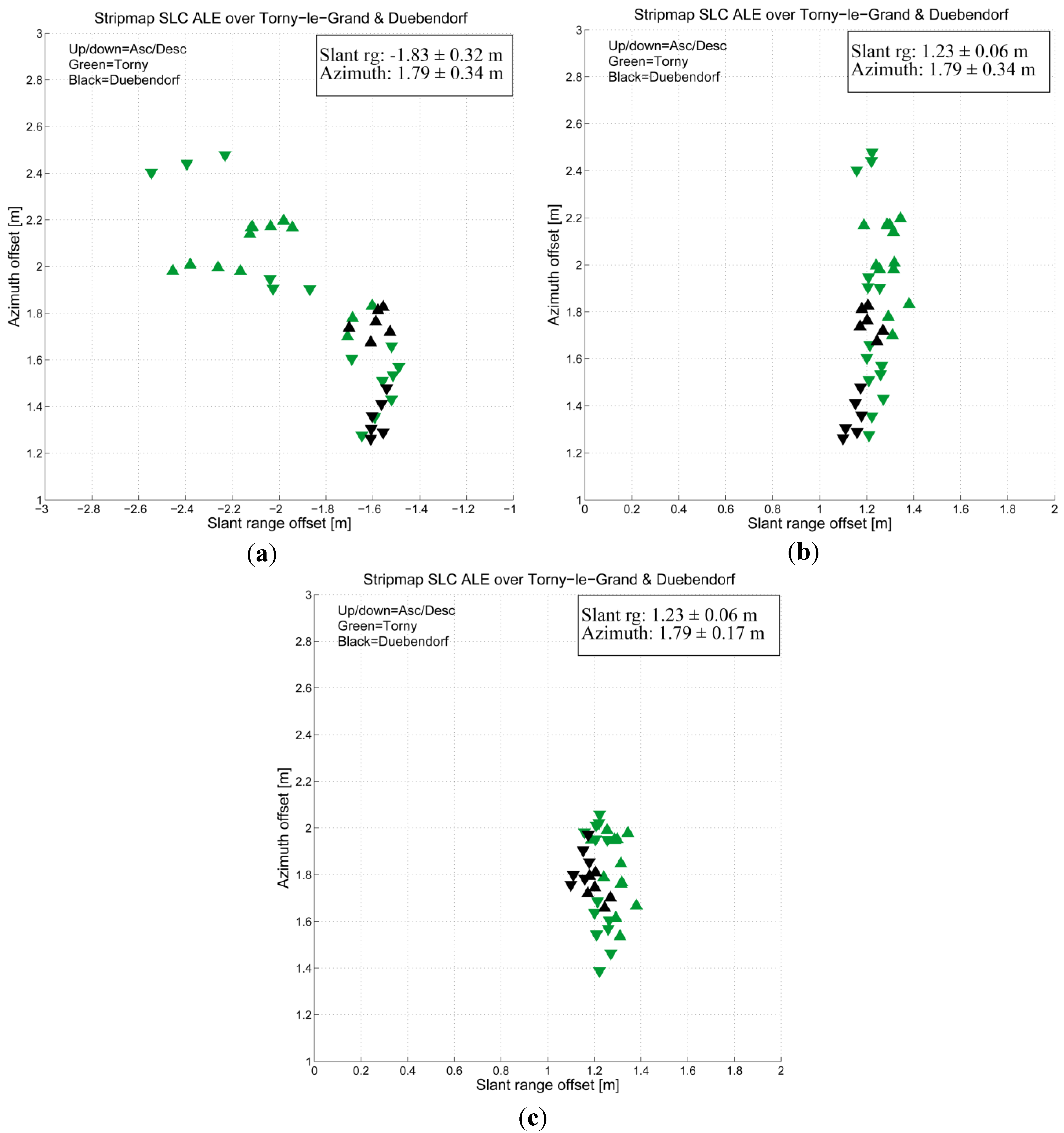
In
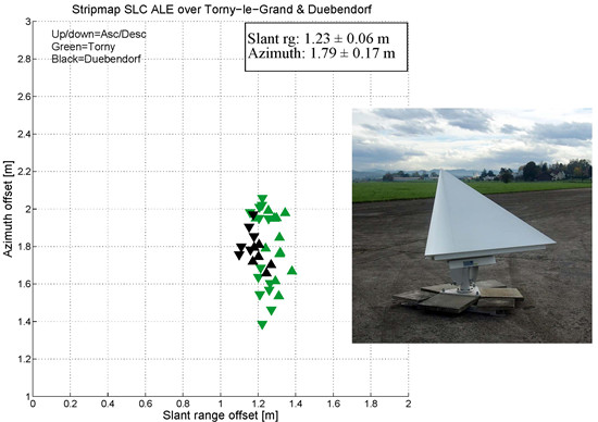
Figure 6, the ALE is shown for three scenarios as a scatterplot for the SM SLC time series over both test sites combined. The slant range ALE is the horizontal axis; azimuth ALE is the vertical axis. For all SM mode ALE plots, the scale and axis extents are the same to facilitate easy comparison. Each green point is a mean ALE value for the CR pair in the case of
Torny-le-Grand; each black point represents a single product over
Dübendorf. Up-pointing symbols are from ascending-orbit acquisitions, down-pointing symbols from descending products. The mean and standard deviation of the point cloud is given for each plot in the inset box.
In
Figure 6a, no atmospheric PD and no bistatic residual corrections were applied. The large spread in range is caused by a variation in the path delay error from product to product, while the azimuth spread largely reflects the variations in the CR positions relative to the scene mid-range (
i.e., the bistatic residual correction). Note that no products from SM beam S1 were available for inclusion in the analysis. The range spread would be expected to be even greater if such products were added to the mix, since the atmospheric path length difference is greatest between beams S1 and S6. Additionally, the diversity of bistatic residual values would increase.
Figure 6b shows the same scatterplot, but includes the PD correction. The range standard deviation has improved six-fold, highlighting the importance of this correction.
Figure 6.
StripMap SLC ALE estimates based on precise state vectors; each point represents a single product over Torny-le-Grand (green) or Dübendorf (black); (a) no path delay or bistatic residual corrections; (b) path delay correction but no bistatic residual correction; (c) path delay and bistatic residual corrections applied. (a) no PD, no bistatic; (b) PD, no bistatic; (c) PD, bistatic.
Figure 6c includes the bistatic residual correction as well, with a corresponding ~two-fold reduction of the spread.
Figure 6c represents the best geolocation result achieved during the calibration phase for S1A: it reflects the extraordinarily high ranging accuracy of the sensor, and an azimuth consistency that is very good as well, although not as consistent as the range. This may partly be due to the coarser azimuth sample spacing in comparison with the slant range sampling. For the S2 beam, the range spacing is ~1.8 m while S6 products have a range spacing of ~3.2 m. In all cases, the azimuth spacing is nearly constant at ~4.1 m. This suggests that the measurement of the CR peak position could be less accurate in the azimuth dimension, as less information might be available for oversampling the raster.
The range and azimuth biases (mean ALE values) estimated from
Figure 6c may be considered calibration biases: their removal from the product timing annotations would center the scatterplot on (0, 0) and increase the mean geolocation accuracy of the delivered products. This change was in fact implemented in the IPF for the slant range bias on 5 May 2015, effectively shifting the mean range ALE to 0 m. Note that since PD has been compensated here, the delivered products would not be as accurate
without PD compensation. However, investigations are underway, with ESA considering how to fully correct for the bistatic effect and even incorporate PD estimates into the product annotations, so that out-of-the-box product geolocation would already provide the best possible accuracy.
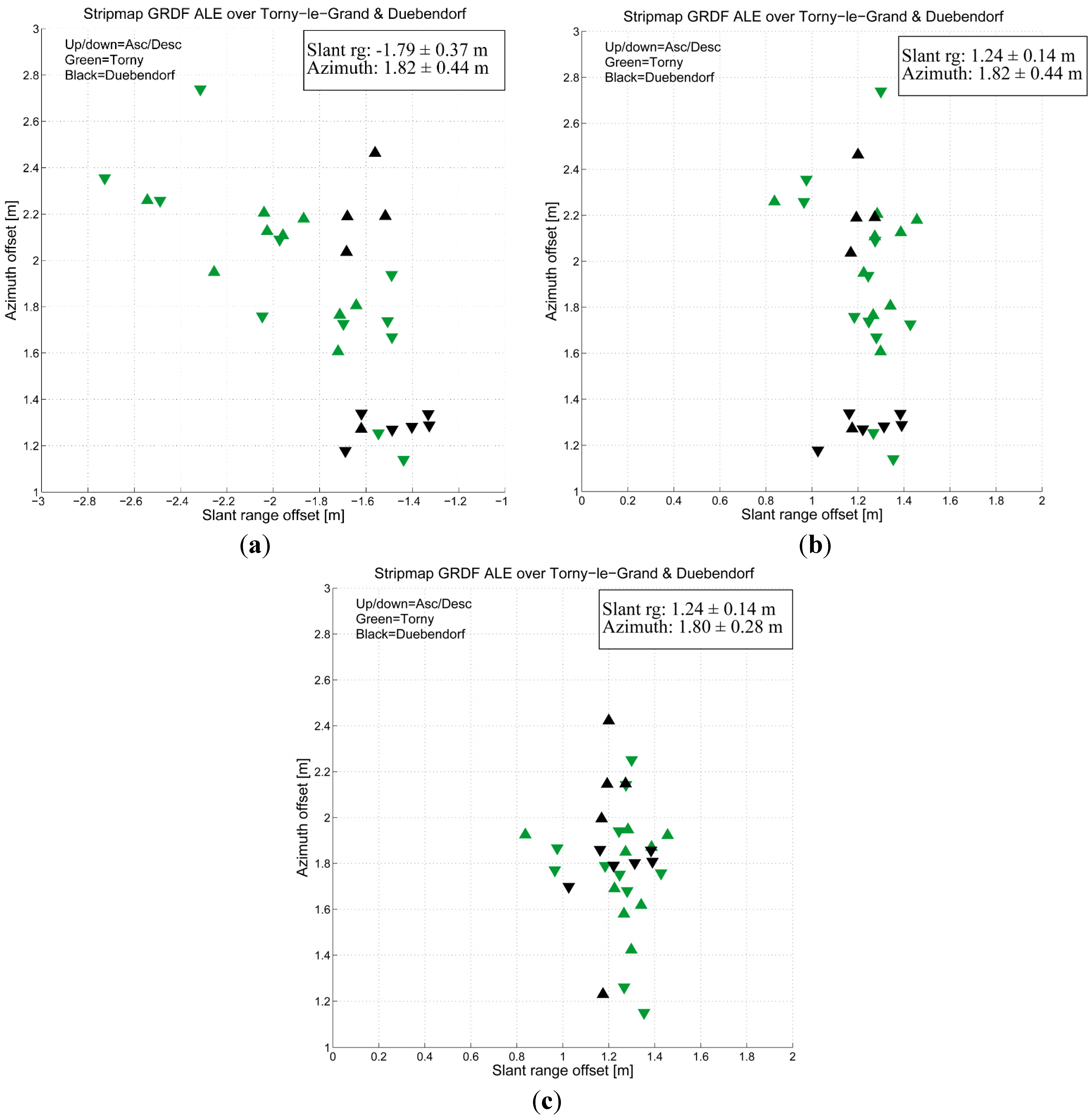
In
Figure 7, the analog of
Figure 6 is shown, but for the corresponding GRDF products. While the effects of the PD and bistatic residual corrections are the same, the best-case ALE standard deviation (
Figure 7c) is not as accurate as the SLC case. This is unsurprising, as GRDF products are further processed via a slant-to-ground-range polynomial, and their SM sample spacing is fixed at 4.0 m in both dimensions, reducing the available range resolution compared with SLC products. More information is lost during the
detection step: the conversion of the complex values to amplitudes. Less information is then available during the oversampling step where the CR peak position is measured in the image raster.
On the other hand, the
mean biases in
Figure 6c and
Figure 7c are nearly identical. This is strong evidence that the slant to ground range processing step does not introduce any unexpected biases itself, and is functioning as planned.
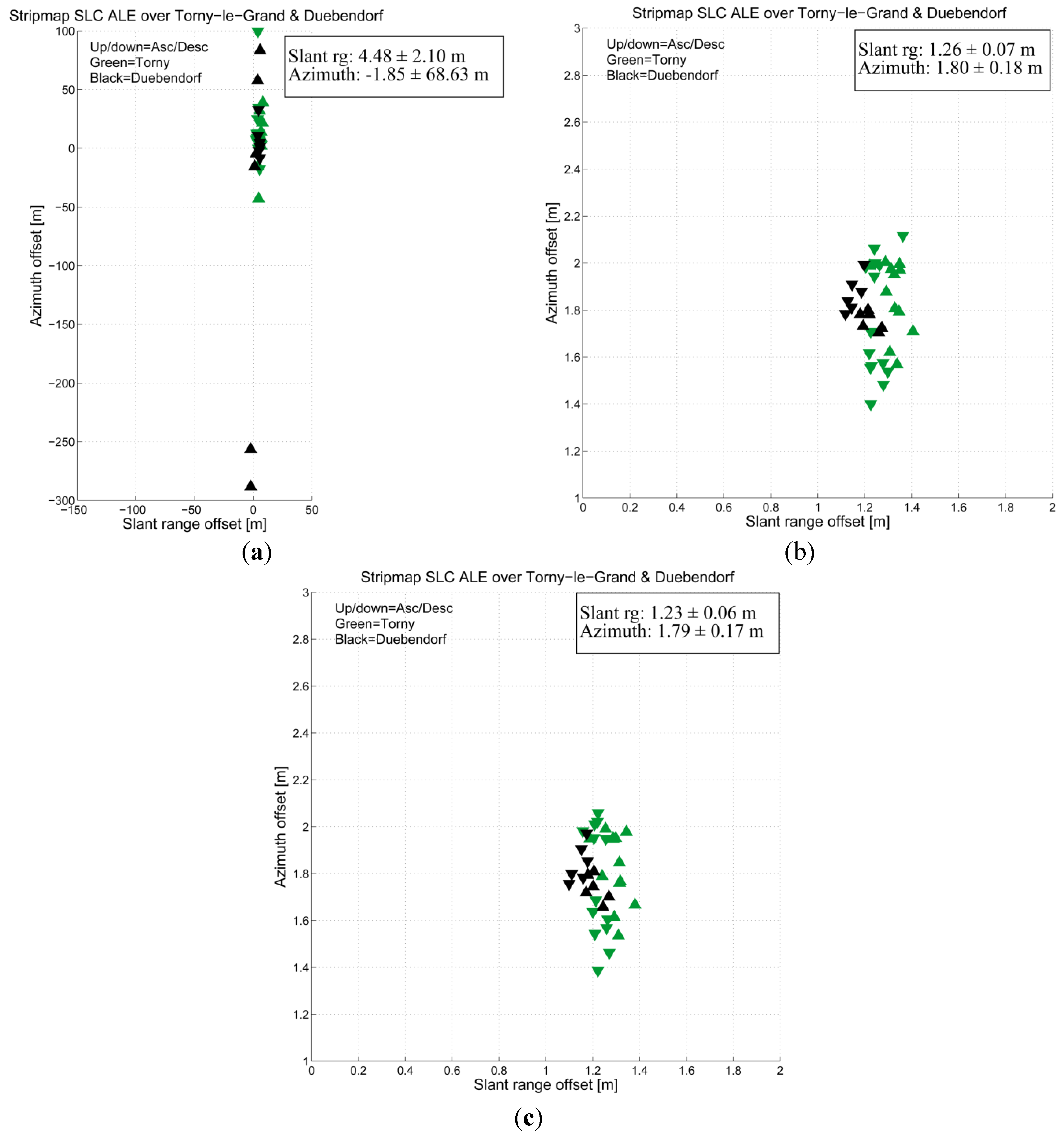
The SM products may provide high ranging accuracy, but to compare the accuracies of the different primary OSV sources, the ALE was estimated in the same way as for
Figure 6c, this time using different OSV sources. A comparison is shown in
Figure 8. In all three cases, orbit interpolation was performed using ESA’s EO_CFI library.
The ALE using predicted OSV files is shown in
Figure 8a. Along-track errors of over 200 m were occasionally observed, probably due to orbit propagation error over the large time interval between file generation (
i.e., when the orbit is propagated) and the actual acquisition, although most values were below ~50 m. Note that predicted OSV files (AUX_ORBPRE) are the only case where the file is generated before the acquisition. Restituted (AUX_RESORB) and precise (AUX_POEORB) files are generated
a posteriori based on GNSS measurements. Much more encouraging is the ALE scatter in
Figure 8b, based on the restituted OSVs. These are available in near-real-time,
i.e., a latency of less than 3 hours after product acquisition. Comparing the restituted with the precise OSV result, which is repeated in
Figure 8c, it is clear that both are nearly equivalent, with only a loss of ~1 cm in the azimuth and range standard deviations in the restituted case. For all but the most time-critical applications, the AUX_RESORB orbit files should therefore be sufficient.
All SM mode products fulfil the accuracy requirement of 2.5 m specified for this mode using near-real-time restituted OSVs (see Tables 7-1 and 7-2 in [
2]). In fact, even the GRDF products without PD or bistatic residual corrections applied (
i.e., the “out-of-the-box” scenario shown in
Figure 7a) meet this requirement.
Figure 7.
StripMap GRDF estimates using precise state vectors; each point represents a single product over Torny-le-Grand (green) or Dübendorf (black); (a) no path delay or bistatic residual corrections; (b) path delay correction but no bistatic residual correction; (c) path delay and bistatic residual corrections applied. (a) no PD, no bistatic; (b) PD, no bistatic; (c) PD, bistatic.
Figure 8.
Comparison of StripMap SLC ALE estimates for different orbital state vector sources; path delay and bistatic residual correction applied in all cases; (
a) predicted; (
b) restituted; (
c) precise (repeated from
Figure 6c). (a) predicted OSVs; (b) restituted OSVs; (c) precise OSVs.
Figure 8.
Comparison of StripMap SLC ALE estimates for different orbital state vector sources; path delay and bistatic residual correction applied in all cases; (
a) predicted; (
b) restituted; (
c) precise (repeated from
Figure 6c). (a) predicted OSVs; (b) restituted OSVs; (c) precise OSVs.
ESA and the geometric calibration team are currently discussing how to best incorporate the calibration results into future products. As mentioned earlier, the mean slant range bias was already incorporated into the IPF on 5 May 2015. It can be expected that product geolocation accuracy will continue to improve, with possible changes to the operational IPF taking atmospheric PD even the bistatic residual error into account.
A comment on the main operational IW mode needs to be made here. Because of the more complex acquisition geometry and product configuration of the TOPS mode products (
i.e., IW and EW), the handling of these products requires extra processing steps in comparison with the SM mode products. These include spectral “deramping” to compensate for the Doppler centroid variations caused by azimuth beam steering, and “debursting”
i.e., merging of the azimuth bursts. At UZH, these steps have until now been nearly completed. At this point, the following can be said:
Ground range detected (GRD) products can be handled in the same way as SM products, but do not contain as much detail as the SLC products from the same acquisitions. Therefore, detailed analyses of these products were not performed.
The wider coverage offered by these two modes comes at the cost of resolution loss, and the deployed ~1 m corner reflectors were only clearly visible in IW products (not EW).
Preliminary geolocation estimates were made by UZH for IW SLC products. However, the measurements were based on detected versions of these products rather than on the native complex SLC samples. As stated above, the use of the complex IW/EW data requires additional processing that has yet to be fully implemented at UZH. Since recent tests revealed differences between ALE estimates made using detected vs. complex rasters, we are confident that our preliminary IW SLC results do not yet fully represent the SLC product quality. Therefore, we chose not to show them here.
With the above considerations in mind, we may nonetheless state that the preliminary IW SLC ALE estimates tentatively confirmed our expectations. The mean ALE corresponded quite well with the SM mode estimates. Improved IW SLC results may be published in the near future.
8. Conclusions
The Sentinel-1A SAR system has set new standards for the achievable geolocation accuracy of comparable spaceborne C-band SAR sensors, with the successful completion of the in-orbit commissioning phase. At the time of this writing, we believe that users can have high confidence in the consistent geometric quality of the level 1 S1A products provided through the data hub. The most significant uncorrected perturbation in these products is currently the atmospheric path delay, which can introduce cross-track (slant range) sample shifts of typically ~3.5 m (i.e., usually ≤ 1 sample, depending on the product type). Based on the results of this study, it can be expected that in the near future, new geolocation correction parameters—including the path delay—will be annotated in S1A image products, simplifying “out-of-the-box” corrections possible if needed. This would further improve the absolute geolocation quality of all standard level 1 SAR image products.
IW SLC results may be published in the future, but for the moment their more complex handling has delayed accurate estimation of their geolocation accuracy. However, the preliminary results (not shown here) were encouraging, with a similar behavior observed as their SM counterparts.
We measured the ALE in the range and azimuth dimensions for SM mode SLC and GRDF products based on a time series of over 40 acquisitions. We performed our analysis using two separately surveyed test sites and S1A SM beams S2 through S6. Considering the very good correspondence between the ALE estimates for the various beams and surveyed reflectors, we can conclude that our atmospheric PD model is working correctly.
Both range and azimuth already exhibit geolocation consistency well within the sub-sample level (as reflected by the ALE standard deviations) when external perturbations are accounted for. For SM SLC the values are 6 cm in range and 17 cm in azimuth (better than ~1/30th of a sample). SM GRDF consistency is 14 cm in range and 28 cm in azimuth (better than ~1/15th of a sample).
The remaining azimuth bias (mean azimuth ALE) of ~1.8 m for both types of SM products may possibly be influenced by a combination of (a) instrument timing mismatches (small difference between GPS and SAR instrument time); (b) orbital state vector estimation in ITRF; (c) orbital state vector interpolation accuracy; (d) satellite center of mass
vs. SAR antenna phase center position; (e) uncertainties inherent in the azimuth time stamp annotations caused by quantization of the clock rate (e.g., for TerraSAR-X this effect contributes up to 6.5 cm azimuth error [
21]); or (f) a bias in the relativistic Doppler correction for along-track motion. These potential influences may be subject to future studies in order to even further improve the already remarkable S1A geolocation accuracy.


