Incorporating Endmember Variability into Linear Unmixing of Coarse Resolution Imagery: Mapping Large-Scale Impervious Surface Abundance Using a Hierarchically Object-Based Spectral Mixture Analysis

Abstract

As an important indicator of anthropogenic impacts on the Earth’s surface, it is of great necessity to accurately map large-scale urbanized areas for various science and policy applications. Although spectral mixture analysis (SMA) can provide spatial distribution and quantitative fractions for better representations of urban areas, this technique is rarely explored with 1-km resolution imagery. This is due mainly to the absence of image endmembers associated with the mixed pixel problem. Consequently, as the most profound source of error in SMA, endmember variability has rarely been considered with coarse resolution imagery. These issues can be acute for fractional land cover mapping due to the significant spectral variations of numerous land covers across a large study area. To solve these two problems, a hierarchically object-based SMA (HOBSMA) was developed (1) to extrapolate local endmembers for regional spectral library construction; and (2) to incorporate endmember variability into linear spectral unmixing of MODIS 1-km imagery for large-scale impervious surface abundance mapping. Results show that by integrating spatial constraints from object-based image segments and endmember extrapolation techniques into multiple endmember SMA (MESMA) of coarse resolution imagery, HOBSMA improves the discriminations between urban impervious surfaces and other land covers with well-known spectral confusions (e.g., bare soil and water), and particularly provides satisfactory representations of urban fringe areas and small settlements. HOBSMA yields promising abundance results at the km-level scale with relatively high precision and small bias, which considerably outperforms the traditional simple mixing model and the aggregated MODIS land cover classification product.

1. Introduction

The global urbanization process exerts great influence over various socioeconomic activities, public health, and global environmental change [1,2,3]. Examples include the urban heat island phenomenon, global precipitation patterns, global warming, etc. [4,5,6]. This process results in the increase of impervious surface coverage [7,8], such as roads, parking lots, buildings, drive ways, and sidewalks. With different climate and socioeconomic influences, the relationship between landscape changes in the urbanization process and global environmental change is still not very explicit [1,9]. As an important representation of the anthropogenic disturbance on the Earth’s surface, it is of great necessity to accurately map regional/global impervious surface coverage to better understand the impacts of urbanization on environmental change [10,11,12,13,14].

There are several different sources of coarse resolution data for large-scale land cover mapping, e.g., Global Land Cover 2000 (GLC2000) [15], MODIS Land Cover 500 m (MOD500) [11]; MODIS Land Cover 1 km (MOD1K) [10], Global Rural-Urban Mapping (GRUMP) [16,17], etc. By comparing the resolutions of these products, it is found that 1-km satellite imagery becomes an important data resource for mapping large-scale land covers. There could be three reasons for its popularity. First, the recently emerged satellite imagery can be used to construct continuous earth observation, and to integrate into well-established modeling for various scientific applications [18,19]. For example, the 1-km resolution of MODIS images can be combined with the historical AVHRR archive for regional and global land cover change detection for biodiversity and ecosystem modeling [20]. Second, 1-km imagery provides a fourfold increase in computational efficiency when compared with its 500-m counterpart for large-scale abundance mapping, particularly when the image processing technique is based on spectral mixture analysis (SMA) running in an iterative fashion, e.g., multiple endmember SMA (MESMA) [21], and endmember bundles [22]. Third, such a resolution is suggested as a favorable scale in regional and global urban observation studies [4,8,23].

In terms of the image processing methods for creating land cover products, fractional land cover datasets at the same resolution are able to preserve spatial and quantitative land composition information at the subpixel level [8,24]. Therefore, in contrast to the lack of spatial details with the 1-km classification maps, subpixel abundance maps have an advantage over classified images. SMA [25,26,27] has been extensively used with 500-m satellite imagery for estimation of fractional land covers or landforms in different natural environments. Examples include the Brazilian Amazon [13], desert [28], and structurally complex savanna [29]. This technique, however, has rarely been applied at 1-km resolution (with the exceptions of the works of fire properties [30] and global vegetation [31]). It is due mainly to two long-lasting technical difficulties in SMA. First, it is extremely challenging to extract homogeneous surface covers (also known as endmembers) for SMA by using existing endmember extraction methods at such a scale. This difficulty originates from the mixed pixel problem of low resolution imagery with a coarse pixel size. In particular, urbanized areas include mixtures of various and fragmented urban land covers (e.g., different manmade materials, and vegetation species), urban impervious surface endmembers are almost impossible to extract from imagery in heterogeneous urban environments at the km-level scale [8,12,13,32,33]. Second, endmember variability is also a challenge in SMA. In particular, the large image footprint of coarse resolution imagery inevitably encompasses a variety of land covers over a large geographic coverage, which intensifies endmember variability for large-scale subpixel mapping. Endmember variability is regarded as the most significant source of error in SMA [21,22,34]. Two major categories of endmember variability are highlighted [35,36], including the between- and within-class variations. The former refers to the spectral confusions among different land cover classes (e.g., bare soil/water and urban impervious surface), while the latter implies the spectral contrasts within the same land cover types (e.g., concrete and asphalt in the urban impervious surface class, and different vegetation species). A variety of methods have been developed to address the issue of endmember variability [34], for example, MESMA [21], endmember bundles [22,37], spatially adaptive SMA (SASMA) [36], automated SWIR unmixing [38], etc. Although endmember variability exists in satellite imagery at most spatial resolutions [39], endmember variability has rarely been investigated with coarse resolution imagery for heterogeneous urban environments in the literature.

The major objective of this research is to generate accurate subpixel urban land cover maps over a large study area. This is expected to be achieved by addressing two major technical difficulties in SMA, including (1) to derive endmember signatures at the km-level scale for spectral unmixing of coarse resolution imagery; and (2) to mitigate the severe effects of endmember variability in an attempt to improve the estimation accuracy of land cover abundance. To reach these goals, a new image processing algorithm, hierarchically object-based SMA (HOBSMA), was proposed to incorporate spatial, temporal, and spectral information into linear spectral unmixing for mapping subpixel urban impervious surface distribution at the 1-km resolution.

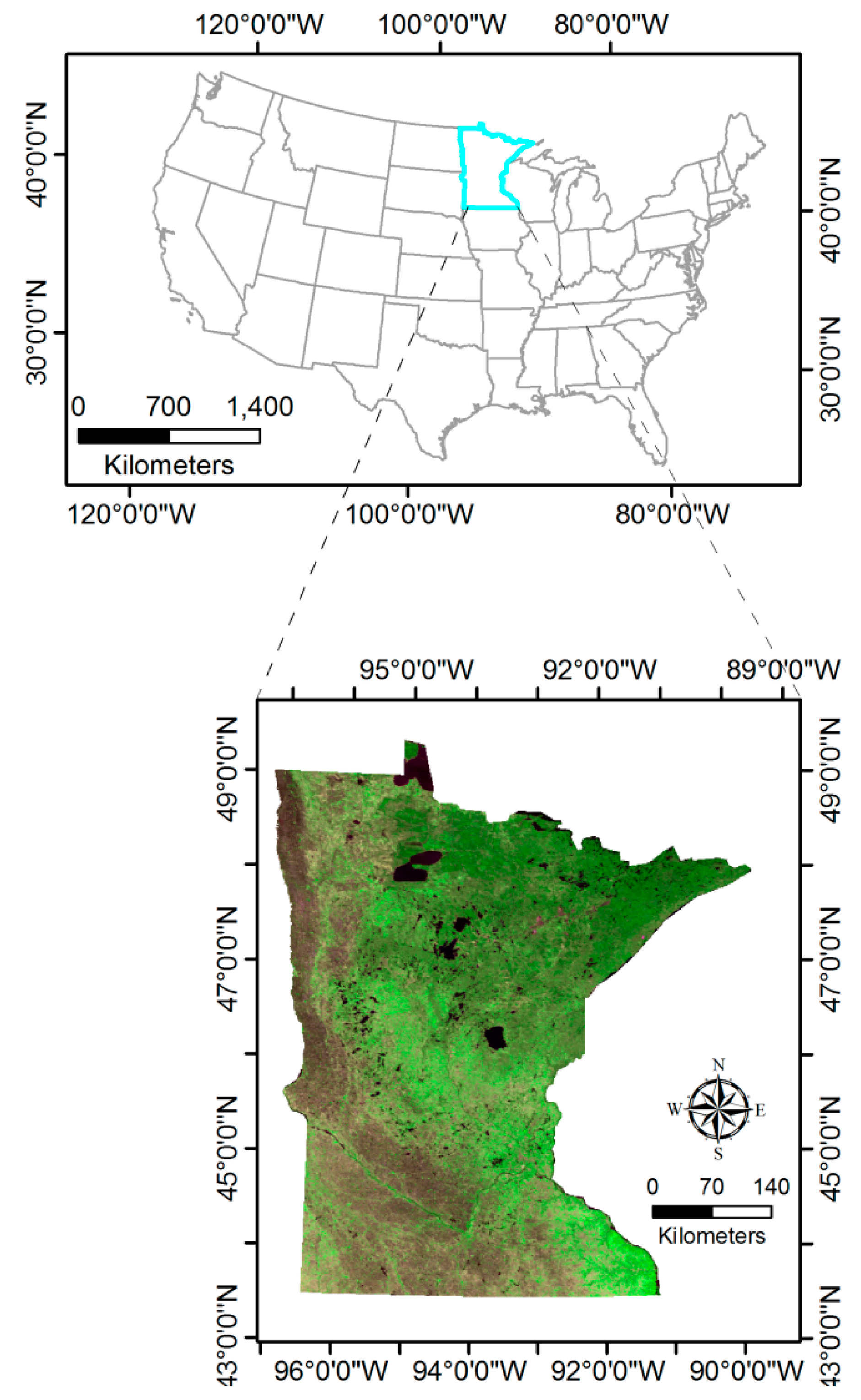
2. Study Area and Data

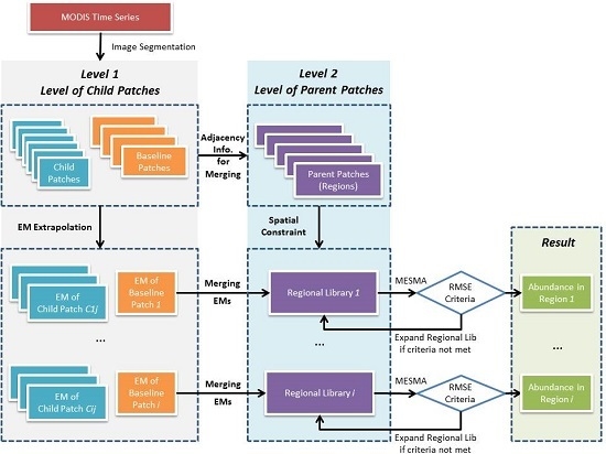
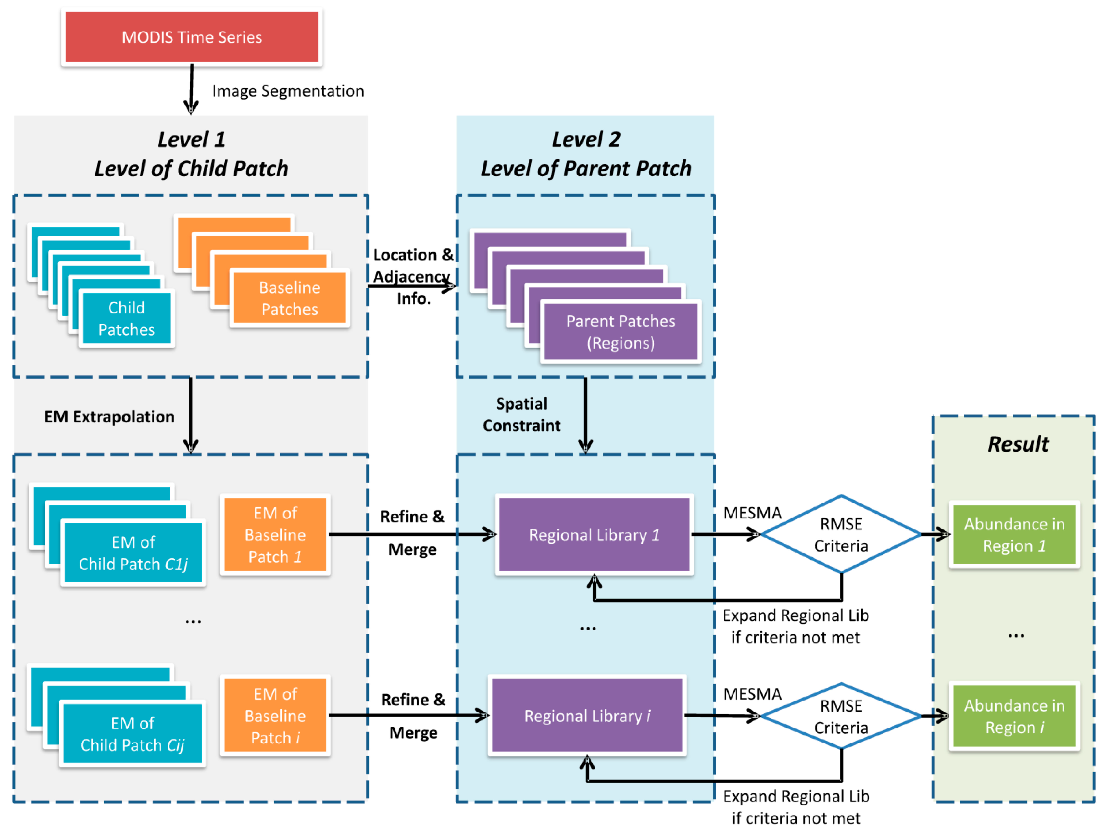
This study was conducted in the state of Minnesota in the United States (see Figure 1) over an area of approximately 225,181 km². A great number of land covers with distinct spectral features appear over such a large geographical area. For example, a large amount of agricultural lands and lakes throughout the state result in numerous mixed pixels, particularly both bare soil and water are spectrally similar to urban impervious surfaces. With such a severe mixed pixel problem, Minnesota therefore is intentionally chosen to examine the effectiveness of the proposed algorithm to address the endmember variability issue as well as the endmember extraction issue. According to the 2006 national land cover datasets (NLCD) product [40], a variety of land cover classes exist in Minnesota, including developed and populous urbanized areas (e.g., the Twin Cities of Minneapolis and Saint Paul), small settlements (e.g., small towns and villages in suburban areas), and sparsely populated rural areas featuring lakes, rivers, agricultural lands, forests (e.g., conifer, deciduous, and mixed), wetlands, and grassland (e.g., tallgrass prairie).

MODIS 1-km Nadir bidirectional reflectance distribution function (BRDF)-Adjusted Reflectance (NBAR) time-series images in 2006 were downloaded from the U.S. Geological Survey (USGS) website. These images were taken on 23 April, 17 May, 2 June, 28 July, 29 August, 30 September, and 17 November, respectively. With preprocessed atmospheric and view angle correction, no further corrections were performed with these images. Both of the 30-m 2006 NLCD land cover and percent impervious surfaces products were used as ground truth for accuracy assessment. All seven original MODIS images (each with seven VSWIR bands) were stacked to generate a scene of MODIS composite with 49 bands. For comparison purposes, a scene of 500-m MCD12Q1 land cover classification product was downloaded. All images were subset and re-projected to Universal Transverse Mercator (UTM) Zone 18 North with the WGS84 datum.

Figure 1. Study area of Minnesota, United State shown in a natural color MODIS composite.

Figure 1. Study area of Minnesota, United State shown in a natural color MODIS composite.

3. Methodology

To address endmember variability with MODIS 1-km imagery, the solution proposed in this paper is to divide the image into several homogeneous regions using image segmentation, followed by solving for region-specific endmembers in each region to construct regional spectral library for linear unmixing. Based on this idea, HOBSMA consists of three major steps: (1) image segmentation at two hierarchical levels; (2) endmember signature extrapolation and regional spectral library construction; and (3) MESMA implementation. A flowchart of this algorithm is provided in Figure 2.

Figure 2. The flowchart of HOBSMA.

Figure 2. The flowchart of HOBSMA.

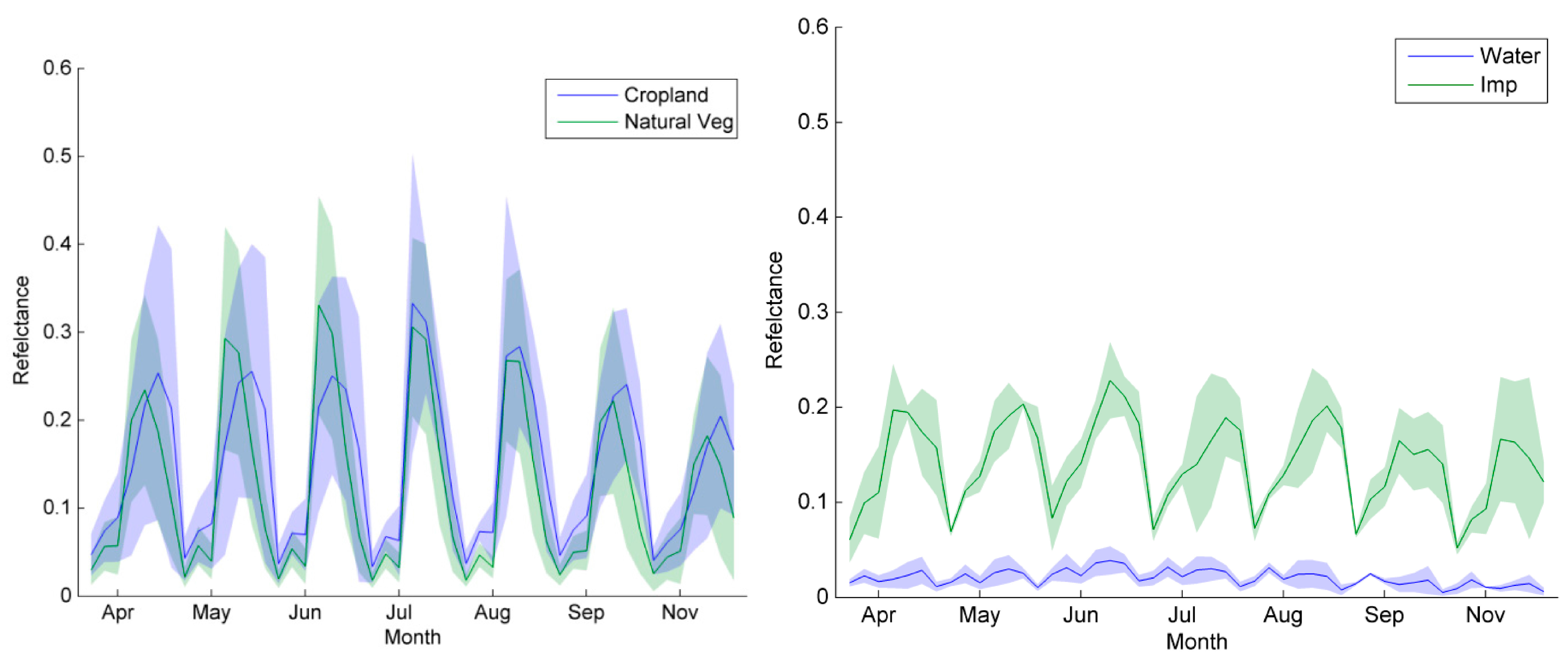
3.1. Endmember Determination with 1-km MODIS Imagery Prior to Unmixing

It is important to determine appropriate types and number of endmembers in linear spectral unmixing [21]. On one hand, the use of excessive endmembers is very sensitive to noise from instruments and atmospheric conditions, which increases the risk of endmember multicollinearity in SMA, and accordingly leads to inaccurate abundance results [41]. On the other hand, with insufficient endmembers, fractional land cover estimates will include unmodeled endmembers, which could be unreliable in any applied practice [21]. In this research, the type and number of endmembers were determined based on both the International Geosphere-Biosphere Program (IGBP) land cover classification system [42,43,44] and the actual land cover conditions in Minnesota. IGBP land cover inventory is a scheme designed for regional/global land cover classification adopted by NASA’s Earth Observing System (EOS) to generate MODIS-based products for global change studies. In this scheme, 17 land cover classes are aggregated into three major categories: natural vegetation, developed and mosaic lands, and non-vegetated lands [45]. Natural vegetation consist of 11 land cover classes, including 5 types of forests, 2 types of shrub land, 2 types of savannas, and one for grasslands and wetlands each. Developed and mosaic lands are composed of three categories including cropland, cropland/natural vegetation mosaic, and urban areas. Non-vegetated lands include barren, permanent snow and ice, and water.

In the case of Minnesota, endmember types were determined based on these three general IGBP classes. For all natural land cover categories, natural vegetation (excluding savanna) is representative and therefore should be considered as one of the endmembers. Note that, as the goal of this study is for land cover abundance estimation as opposed to simple hard classification, urban vegetation (such as urban forest, trees, and lawns) should also be included in this natural vegetation endmember. For developed and mosaic lands, this essentially means a mixed class of various land covers. According to the different levels of anthropogenic impacts in this study area, two endmember types can be identified from this class: urban impervious surface and cropland/planted lands. In regards to non-vegetated lands, since barren lands, permanent snow, and ice are rarely found in Minnesota while there are a large number of lakes with different sizes throughout this study area, this class of non-vegetated lands can be simplified by water. It is worth noting that water is rarely considered as an endmember in most current urban mapping (e.g., Ridd’s Vegetation Impervious surface-Soil (V-I-S) model) [46], the reason for which is twofold. First, as a low albedo land cover, the spectral confusion between water and dark impervious surface results in inaccurate abundance estimates of urban impervious surface. Second, water does not always exist in all urban areas, especially for a relatively small study area (e.g., at the city level). This assumption, however, is not true for regional/global mapping with a large study area. For example, lakes with various sizes are unevenly distributed throughout Minnesota, which results in the severe mixture of water and other land cover classes in the 1-km pixels. Moreover, it is almost impossible to remove all water-contaminated pixels. As such, water should also be considered. Overall, four endmembers were used for linear unmixing, including natural vegetation, cropland/planted lands, urban impervious surface, and water.

3.2. Image Segmentation at Hierarchical Levels: Retrieving Spatial Information of Patches

HOBSMA was performed at two hierarchical levels: the first level provides spatial constraints to extrapolate endmember signatures, and the second level provides spatial constraints to construct regional spectral libraries for iterative unmixing. The focal point here is the generation of parent patches to retrieve spatial information of image patches as spatial constraints, and the complete procedure of regional library construction will be introduced in the next subsection.

At the lower hierarchical level, the image was first segmented into a series of statistically different patches. It is expected that endmembers could be extrapolated in each patch, by which sufficient endmembers can be collected to accommodate endmember variability. The image segmentation was implemented by a new object-based image analysis (OBIA) technique called statistical region merging (SRM) [47]. SRM was originally developed in the fields of computer vision, machine learning and pattern analysis [47], and has been recently applied to high-resolution image classification in the remote sensing community [48,49,50]. This algorithm starts with small initial image regions and merges them to generate the final segmentation based on a statistical analysis. Two core criteria were proposed for determining optimal image regions [47]:

(1)

Pixels in each optimal region should have the same expectation.

(2)

Adjacent optimal regions should have a statistically different expectation for at least one band.

To meet these requirements, the dissimilarity of the pairs of adjacent pixels in a 4-connexity neighborhood was first measured and sorted in ascending order by a simple gradient function, which can be formulated as follow [47].

$$\text{D}\left(\text{p},{\text{p}}^{\prime }\right)=\text{max}\left|{\text{p}}_{\text{a}}^{\text{′}}-{\text{p}}_{\text{a}}\right|$$

(1)

where $p_a^{\prime }$ and $p_a$ are pixels values of a pair of adjacent pixels in band a. Adjacent pixels are defined as 4-connexity neighbors that are either horizontally or vertically located. This order is then traversed for any pairs. When two pixels of a pair belong to different initial image segments, a merging test is then performed, which can be expressed as follows [47].

$$P\left(R,R^{\prime }\right)=\{\begin{array}{c}true, if\left|\overline{R^{\prime }}-\overline{R}\right|\le \sqrt{b^2\left(R\right)+b^2\left(R^{\prime }\right)}\\ false, otherwise\end{array}$$

(2)

where $b\left(R\right)=g\sqrt{1/\left(2Q\left|R\right|\right)\text{ln}\left({ℛ}_{\left|R\right|}/\delta \right)}$; R is a region of an image I; $\overline{R}$ is the observed average in region R; ${ℛ}_m$ is the set of regions with m pixels in I; δ is the maximum probability that the test result is false, which usually is set as a very small number; and Q is a parameter that quantifies the complexity of the image and the generality of the statistical model, and controls the coarseness of the segmentation. These segments will be merged if the test result is true. Readers are referred to [47] for more details of the sorting function and the merging predicate. This algorithm is able to cope with occlusion and noise corruption, and provide fast and reliable segmentation results [48,49,50]. All the partitioned segments derived from SRM in this step are referred to as “child patch”.

Based on the classic MESMA work [21] and the spatial autocorrelation theory [51], the constructions of several regional spectral libraries are expected. This is because each regional library can be regarded as a subset of the global spectral library, and the computational cost can be greatly reduced by using a regional library with fewer but region-specific endmembers [52]. To achieve this goal, at the upper hierarchical level, the extent of such image regions (hereafter “parent regions”) was designed to spatially constrain the construction of regional library. Parent regions are defined as a large image segment that consists of a child patch obtained from Level 1 with a relatively large geographic area (hereafter the “baseline child patch”) and a number of adjacent child patches with a much smaller geographic area. The geographic area of each child patch was calculated and sorted in descending order. If the cumulative area of the largest N child patches is more than 90% of the study area, these N top-ranked child patches were selected as the baseline child patches. Accordingly, N parent regions were derived through respectively merging small child patches into their adjacent baseline child patch using a flood-fill algorithm of morphological reconstructions [53]. The spatial information (location and adjacency) of parent patches will be further employed to construct N regional spectral libraries.

3.3. Regional Library Construction: Endmember Extrapolation, Refinement and Aggregation

The resultant child patches of Level 1 are spectrally distinct from their neighboring segments, and most pixels inside have similar spectral features. Child patches are likely to be dominated by relatively homogeneous land covers with similar biophysical properties, for example, the same vegetation species, soil types, lakes, or built-up areas, etc. Endmembers were first extrapolated in each child patch by using a least squares solution (LSS) technique with known abundance knowledge of sample pixels [8,54]. Two stratified random sampling rules were used for extrapolation in each child patch based on their areal information. First, for small child patches whose patch size is less than or equal to 20 km² (i.e., 20 pixels), 10 random samples were used in each small patch. Second, for a large child patch with a geographic area larger than 20 km², 20 random samples were assigned to each large child patch. After deriving stratified sample pixels, the LSS technique was employed to solve for endmember signatures in each patch with known fractions and spectra of sample mixed pixels, which can be formulated as follows:

$$E=S{F}^T{\left(F{F}^T\right)}^{-1}$$

(3)

subject to

$$E_i\ge 0,E_i\le 1\forall i$$

(4)

where E is the matrix of target endmember spectra; S is a spectral vector of a mixed pixel; F is a vector of known endmember abundance of sample pixels. Impervious surface abundance of sample pixels can be obtained directly from the aggregated 2006 NLCD percent impervious surface data. Similarly, the abundance knowledge of water and cropland/planted lands can also be derived from the 2006 NLCD land cover classification data (class code 11 for water, and 82 for cropland/planted lands). For simplicity, each NLCD land cover pixel is regarded as a homogeneous pixel. Their fractions can be respectively calculated by the aggregated geographical area of the target land cover, divided by 1 km² of the MODIS pixel area. The abundance of natural vegetation is then derived by the subtraction of abundances of impervious surfaces, cropland, and water from one. Note to avoid confusion over terms, the samples for endmember extrapolation are referred to as calibration samples, while the samples used for estimation accuracy assessment are referred to as validation samples. It is also worth noting that the use of NLCD in this pilot study is simply because the NLCD dataset is easy to access. There are also a number of similar medium resolution land cover products across the world, such as the Corine land cover product in Europe, and the global land cover product with a 30 m resolution produced by National Administration of Surveying, Mapping and Geoinformation (NASG) of China. All these products could be incorporated into the proposed method to support timely update of land cover abundance mapping.

These extrapolated endmember signatures were further refined to ensure their validity for unmixing. NDVI on each acquisition date was calculated for each resultant endmember signature by the following formula [55].

$$NDVI=\left({\rho }_{NIR}-{\rho }_{red}\right)/\left({\rho }_{NIR}+{\rho }_{red}\right)$$

(5)

where ${\text{ρ}}_{NIR}$ and ${\text{ρ}}_{red}$ are the reflectance of near infrared and red wavelengths, respectively.

Following the method in [36], if an endmember does not meet any of the following criteria, it will not be further included in a regional library. These criteria include a series of empirical NDVI thresholds for different land covers: (1) an endmember of natural vegetation is considered only if its mean NDVI on all acquisition dates is greater than 0.6; (2) an endmember of croplands is considered only if the contiguous count with an NDVI threshold of 0.6 is no more than 3, corresponding to a maximum of 3 months of maturity period of crops; (3) an endmember of urban impervious surfaces is considered only if its mean NDVI on all acquisition dates is less than 0.2; and (4) an endmember of water is considered only if its mean NDVI on all acquisition dates is less than 0.1 [56,57].

After endmember refinement, local spectral libraries with region-specific endmembers were generated with the following two steps:

(1)

Identification: for each parent patch, all child patches that fall inside were identified and refined using NDVI criteria;

(2)

Aggregation: all refined endmembers of these child patches of each parent patch were merged as a spatially constrained regional spectral library.

N regional spectral libraries from N parent region were then constructed.

3.4. MESMA Implementation

After building regional spectral libraries, iterative unmixing and optimal model selection were implemented [21,58]. Instead of using a fraction criterion in classic MESMA, a fully constrained linear spectral unmixing (FCLSU) was iteratively undertaken with different combinations to derive land cover abundances. Two imposed abundance constraints of FCLSU include: abundance sum-to-one constraint (ASC), and abundance non negativity constraint (ANC). FCLSU and its two constraints are expressed as follows:

$$L_{ }=fR+{\epsilon }_{ }$$

(6)

$${\displaystyle \sum }_{i=1}^n{f}_i=1, and f_i\ge 0\forall i$$

(7)

where L is a spectra vector of a mixed coarse pixel; R is the matrix of endmember signatures, f is the target fraction vector; ε is the model residual vector.

As a quantitative indicator of the model fit, RMSE was calculated for each model using the residuals of all bands, which can be calculated as follows:

$$RMSE={({\displaystyle \sum }_{i=1}^d\raisebox{1ex}{${{\epsilon }_i}^2$}\!\left/ \!\raisebox{-1ex}{$d$}\right.)}^{1/2}$$

(8)

where d is the number of image spectral bands; f is the target fraction vector; ${\epsilon }_i$ is the model residual vector of band i; RMSE is the root mean square error. The smaller the RMSE, the better this model fits.

Two criteria were adopted for optimal model selection. The first one is the RMSE criterion, i.e., any model with an RMSE higher than a predefined threshold of 0.025 will not be considered, a method proposed in the classic work of [21]. It is worth noting that if no candidate model with any endmember combination meets this RMSE criterion, the regional spectral library in the proposed HOBSMA can be very flexible and dynamic. Rather than labeling it as an unmodeled pixel, a new and larger regional spectral library will be generated by merging the libraries of all other adjacent parent regions into the current library, and all potential combinations of endmembers in this new library will be re-tested. The second one is the relative decrease (RD) of RMSE with an empirical threshold of 60 [59]. Lower RMSE values are more likely to associate with models corresponding to combinations with more endmembers, which however might not always be true. This indicator was adopted to select the optimal one among three best-fit models with two-, three-, and four-endmember combinations, respectively. If the RD does not exceed the specified tolerance, the model with i-endmember combination will be selected, otherwise the model with i+1-endmember combination will be selected. The RD calculation continues for models with successive combinations until the RD is less than the specified tolerance.

3.5. Comparative Analysis and Accuracy Assessment

For comparative purposes, a simple mixing model (hereafter simple SMA) was performed by using the four identical endmember classes. The extrapolated endmembers from each original child patch at Level 1 were averaged to derive a set of mean endmember spectra. This endmember set was then used throughout the whole image, such that endmember variability was not taken into account. In addition, the 500-m MCD12Q1 land cover product was aggregated to match the pixels of the MODIS 1-km imagery for further comparisons. All pixels in study area (excluding those calibration pixels) were employed for accuracy assessment. This results in over 200,000 validation samples. Since most pixels are located in rural and suburban areas, impervious surface abundance estimates were further examined in less developed and developed areas, respectively [36]. The abundances of all validation samples were calculated with the 2006 NLCD percent impervious surface product by using the same calculation method for those calibration samples. A comparison was carried out by plotting the reference abundance against HOBSMA modeled abundance. Three parameters of the linear regression model of the scatterplot, i.e., slope, intercept and R-squared, were also calculated from this scatter plot. For quantitative accuracy assessment, three evaluation metrics were employed, including root mean square error (RMSE), mean absolute error (MAE) and systematic error (SE, or bias), which can be formulated as follows:

$$RMSE=\sqrt{\frac{1}{N}{\displaystyle \sum }_{i=1}^N{(\widehat{A_i}-A_i)}^2}$$

(9)

$$RMSE=\sqrt{\frac{1}{N}{\displaystyle \sum }_{i=1}^N{(\widehat{A_i}-A_i)}^2}$$

(10)

$$SE=\frac{1}{N}{\displaystyle \sum }_{i=1}^N(\widehat{A_i}-A_i)$$

(11)

where $\widehat{A_i}$ is the urban impervious surface abundance estimates using HOBSMA; $A_i$ is the reference urban impervious surface fraction of pixel i, derived from the aggregated NLCD percent impervious surface data; and N is the total number of samples. Among these three metrics, RMSE and MAE are usually regarded as quantitative precision measurements for the relative error of fractional land cover estimates, while SE is a bias indicator to measure whether an overall upward/downward estimation tendency exist.

4. Results

4.1. Result of HOBSMA Modeled Abundance

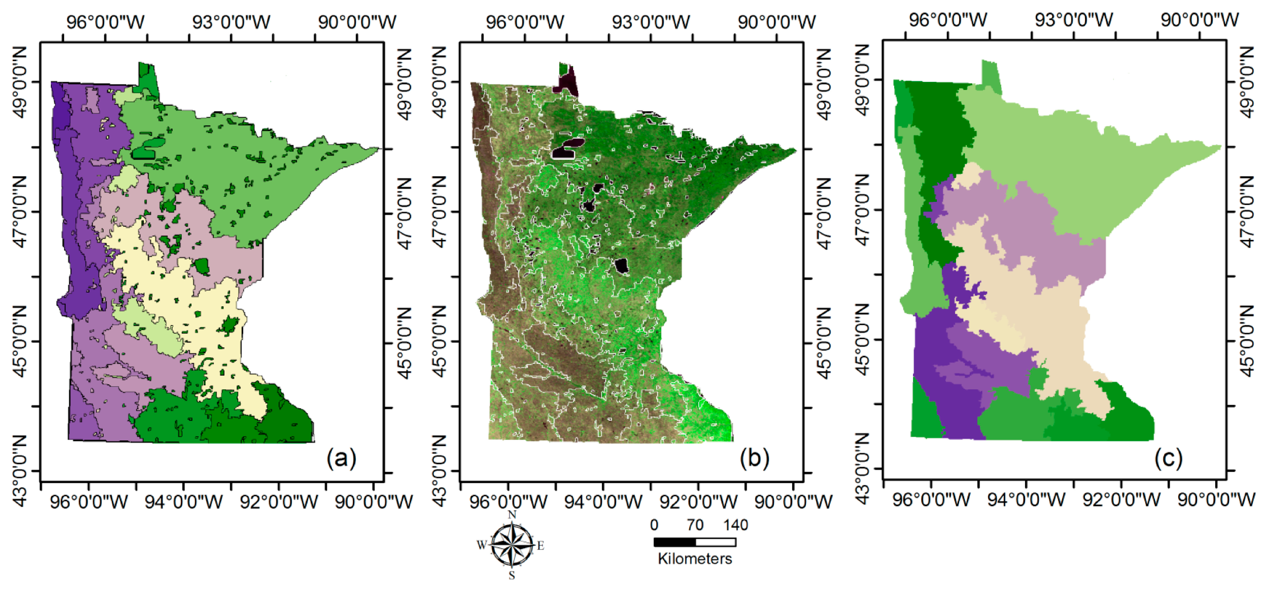
4.1.1. Image Segmentation at Two Hierarchical Levels

The result of image segmentation is shown in Figure 3a. A total of 342 valid child patches with different sizes are shown in different colors. For a better illustration, image objects extracted are white-bordered and overlaid on a composite MODIS image in Figure 3b. It can be observed that those white-bordered image objects correspond to specific land covers clearly. For instance, some small objects are in good agreement with lakes (particularly in central, northern and northeastern parts of the study area), or small patches of grasslands, etc. Figure 3b shows that those larger image objects are in accordance with land covers with similar spectral properties with dark green pixels at the northeastern corner (dominated by woody wetlands, conifer and mixed forests), one with bright green pixels in the central and southeastern part (dominated by deciduous forests or open grassland), and another one with dark brown pixels at the southwestern corner (dominated by cropland/planted lands). Figure 3c illustrates the total of 16 resultant valid parent patches in different colors. These regions were further used as spatial constraints for constructing regional spectral library.

Figure 3. Resultant image segments: (a) original image patches; (b) object boundaries overlaid a composite MODIS image; (c) merged parent regions.

Figure 3. Resultant image segments: (a) original image patches; (b) object boundaries overlaid a composite MODIS image; (c) merged parent regions.

4.1.2. Regional Library Construction and the Variability of Extrapolated Endmembers

Accounting for approximately 1.6% of the study area, a total of 3690 calibration sample pixels were used for the endmember extrapolation in each individual child patch, followed by endmember refinement. Approximately 50% of original endmembers were remained in each regional library by applying the NDVI-based selection criteria. The mean and 95% confidence intervals of extrapolated endmembers of four categories are presented in Figure 4 to illustrate endmember variability across the entire state. As shown with relatively large and overlapped shaded areas, large endmember variations are found to associate with natural vegetation and cropland/planted lands. This observation is not unexpected, since sowing and harvest periods as well as cropping systems (either single or multiple) significantly vary from region to region. Apparent phenological cycles could also be observed with these two land covers, as shown by their seasonal changes (i.e., the changing peak in the near-infrared band of each month in Figure 4). Comparatively, water and impervious surfaces have smaller endmember variations, and their spectra can be clearly discriminated from each other. Endmembers of all child patches that fall inside their parent patch was then aggregated to build regional spectral libraries based on the spatial constraint from their respective parent patch. Consistent with the number of parent regions, 16 regional libraries were obtained. On average, a regional library includes 5 classes of natural vegetation, 4.68 cropland classes, 1.56 classes of impervious surfaces, and 1.38 water classes. Comparing with the global library of traditional MESMA in which all possible endmembers are combined, much fewer endmembers (but more region-specific) were employed in a regional library, by which computational efficiency are likely to significantly increase with comparable accuracy [26].

Figure 4. The mean and 95% confidence intervals of four extrapolated temporal-spectral endmember signatures. All 7 VSWIR wavelengths (with bandwidth ascending) are displayed for each month.

Figure 4. The mean and 95% confidence intervals of four extrapolated temporal-spectral endmember signatures. All 7 VSWIR wavelengths (with bandwidth ascending) are displayed for each month.

4.1.3. Result of Land Cover Abundance by HOBSMA

MESMA was implemented for each parent region by using their respective regional library. The frequency that an endmember was used from adjacent regional libraries varies among endmember types: 2 times for natural vegetation and cropland, 9 for impervious surface, and 4 for water. This may be explained by the different amounts and uneven distributions of land covers throughout the entire state. The resultant abundance results are presented in Figure 5. As the emphasis of the analysis here is placed on urban impervious surface, the HOBSMA-modeled impervious surface abundance map (see Figure 5d) was compared with other basic land cover types (see Figure 5a–c), as well as the abundance map of aggregated 1-km NLCD percent impervious surface fraction product (see Figure 5g). Visual examination finds that the overall pattern of the resultant impervious surface fraction is very close to that of the NLCD reference map: the largest urbanized area in bright grey (i.e., the Twin Cities) can be found commonly in the lower middle part, while other small towns shown in dark grey are scattered over the entire study area. With very little confusions with bare soil in cropland/planted lands in Figure 5b, as well as with water in Figure 5c, reasonable fraction of urban impervious surface can be visually observed in Figure 5d.

An accuracy assessment with quantitative metrics was performed, and a scatterplot was drawn to examine the relationship between the reference and the HOBSMA-modeled urban impervious surface abundance. As illustrated in Figure 6, with most data points clustering around the blue dash reference line, it indicates the regression model has a near 1:1 relationship, as supported by a near-to-one slope (0.815 approaching to 1), small intercept (0.0004 very close to 0) and an adequate R-squared value of 0.687. Accuracy assessment metrics in Table 1 also confirm its promising performance for the entire study area with an RMSE of 3.88%, MAE of 1.13% and SE of −0.16%. In addition to the overall study area, the areas with different levels of impervious surface abundance were analyzed and assessed, i.e., developed areas and less developed areas using 30% as a predefined threshold. Three quantitative accuracy indicators are reported in Table 1. These adequate metrics are also comparable with the accuracy in other existing studies with medium resolution imagery [36,58,60]. Impervious surface abundance is underestimated in both areas (with a SE of −0.11% for less developed areas and −6.78% for developed area). The reason could be that while HOBSMA improves the separation between impervious surfaces and bare soil, the endmember variability issue has not yet been fully addressed and a small number of confusion still remains. However, the underestimation in less developed areas is not very severe, and does not have a significant impact on the total accuracy.

Figure 5. The HOBSMA modeled 1-km land cover abundance maps of (a) natural vegetation; (b) cropland; (c) water; (d) impervious surface. For comparison purposes, impervious surface fractions were derived by using (e) simple SMA; (f) the aggregated 1-km MCD12Q1; and (g) the aggregated 1-km NLCD product (as the reference map).

Figure 5. The HOBSMA modeled 1-km land cover abundance maps of (a) natural vegetation; (b) cropland; (c) water; (d) impervious surface. For comparison purposes, impervious surface fractions were derived by using (e) simple SMA; (f) the aggregated 1-km MCD12Q1; and (g) the aggregated 1-km NLCD product (as the reference map).

Figure 6. Scatterplot comparison between reference and modeled fraction of impervious surface using (a) HOBSMA; (b) simple SMA; and (c) the aggregated 1-km MCD12Q1 data.

Figure 6. Scatterplot comparison between reference and modeled fraction of impervious surface using (a) HOBSMA; (b) simple SMA; and (c) the aggregated 1-km MCD12Q1 data.

Table 1. Comparison of accuracy assessment metrics among three maps.

Method	Sample Area	RMSE (%)	MAE (%)	SE (%)
HOBSMA	Overall	3.88	1.13	−0.16
	Less Developed (<30%)	3.65	1.06	−0.11
	Developed (≥30%)	15.70	11.57	−6.78
Simple SMA (4 EMs)	Overall	5.13	1.87	0.57
	Less Developed (<30%)	4.88	1.76	0.69
	Developed (≥30%)	18.93	16.49	−15.25
Aggregated 1-km MCD12Q1 data	Overall	5.28	1.13	−0.07
	Less Developed (<30%)	3.88	0.85	−0.29
	Developed (≥30%)	41.46	36.94	29.10

Table 1. Comparison of accuracy assessment metrics among three maps.

Method	Sample Area	RMSE (%)	MAE (%)	SE (%)
HOBSMA	Overall	3.88	1.13	−0.16
	Less Developed (<30%)	3.65	1.06	−0.11
	Developed (≥30%)	15.70	11.57	−6.78
Simple SMA (4 EMs)	Overall	5.13	1.87	0.57
	Less Developed (<30%)	4.88	1.76	0.69
	Developed (≥30%)	18.93	16.49	−15.25
Aggregated 1-km MCD12Q1 data	Overall	5.28	1.13	−0.07
	Less Developed (<30%)	3.88	0.85	−0.29
	Developed (≥30%)	41.46	36.94	29.10

4.2. Comparative Analysis

4.2.1. Comparisons with Simple SMA

The performance of HOBSMA was compared with that of simple SMA (see Figure 5e). Since the limitations of SMA are well-known, the key points of comparative analysis were summarized as follows:

(1)

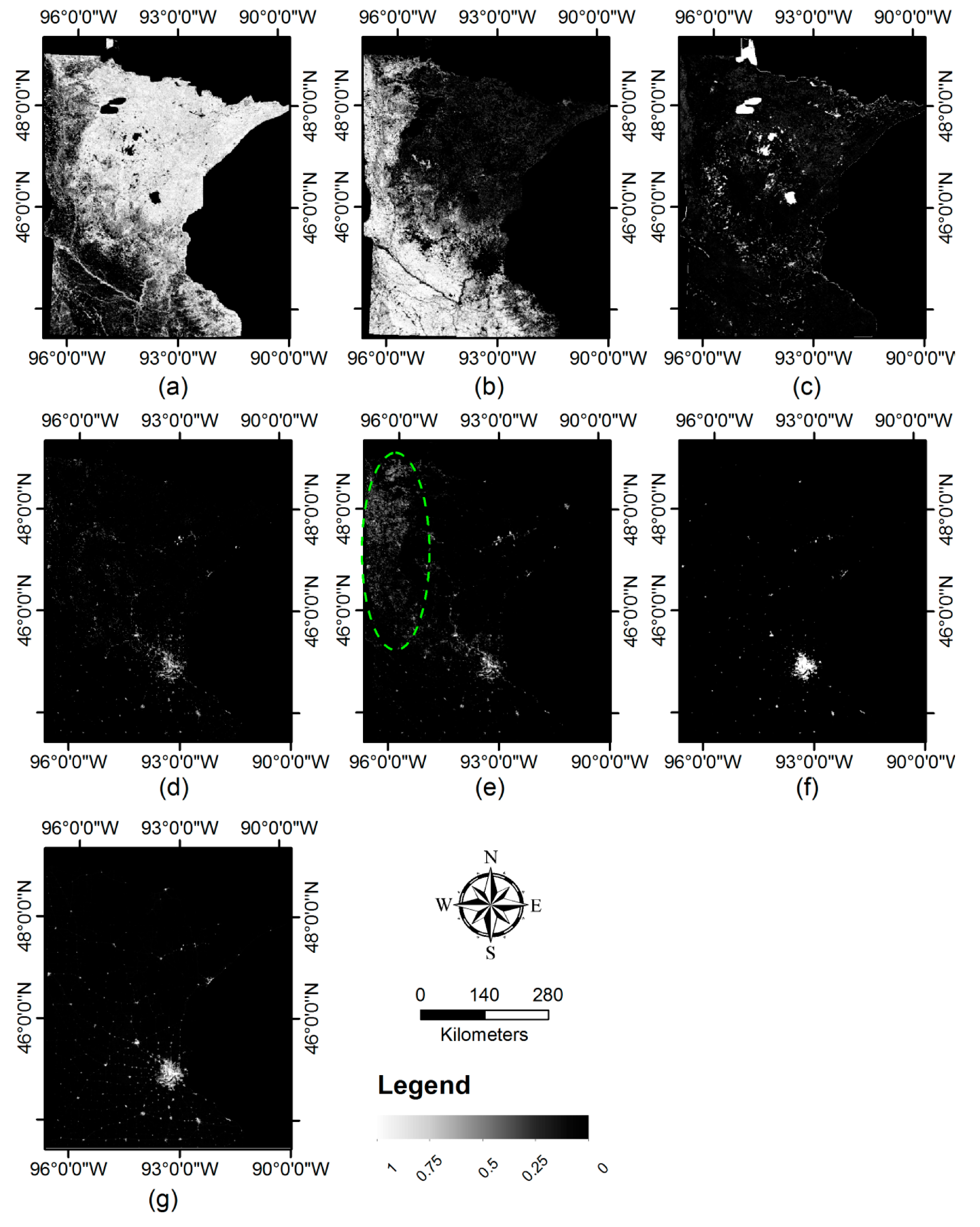
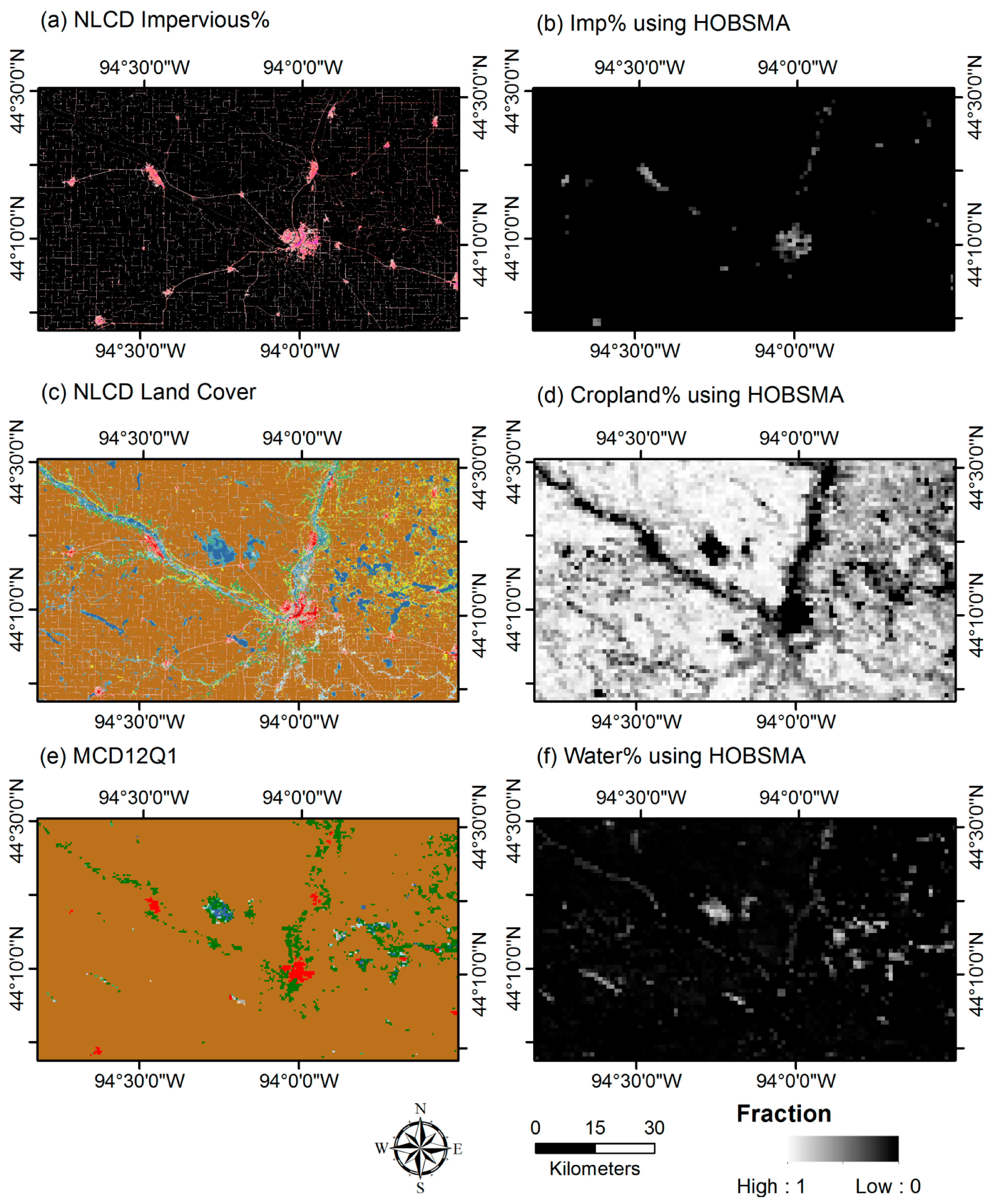
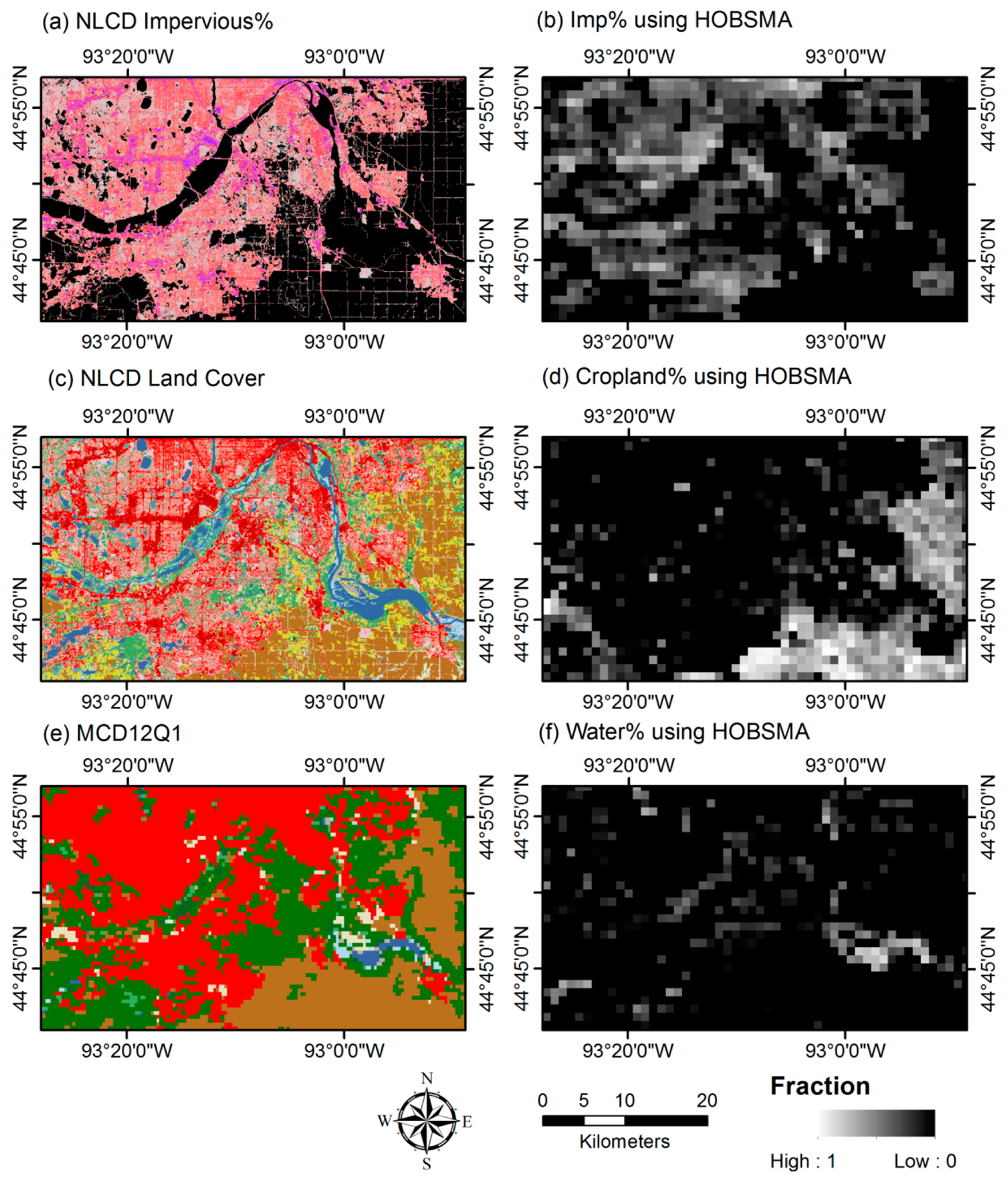
Visual comparison finds that severe underestimations can be found in the major urbanized area (particularly the much darker grey pixels in the Twin Cities area) as well as in suburban settlements, and that overestimations can be discerned in croplands in northwest Minnesota (see the grey pixels inside the green dashed ellipse in Figure 5e). Similar confusions with bare soil in croplands, however, can hardly be noticed with HOBSMA in Figure 5d.

(2)

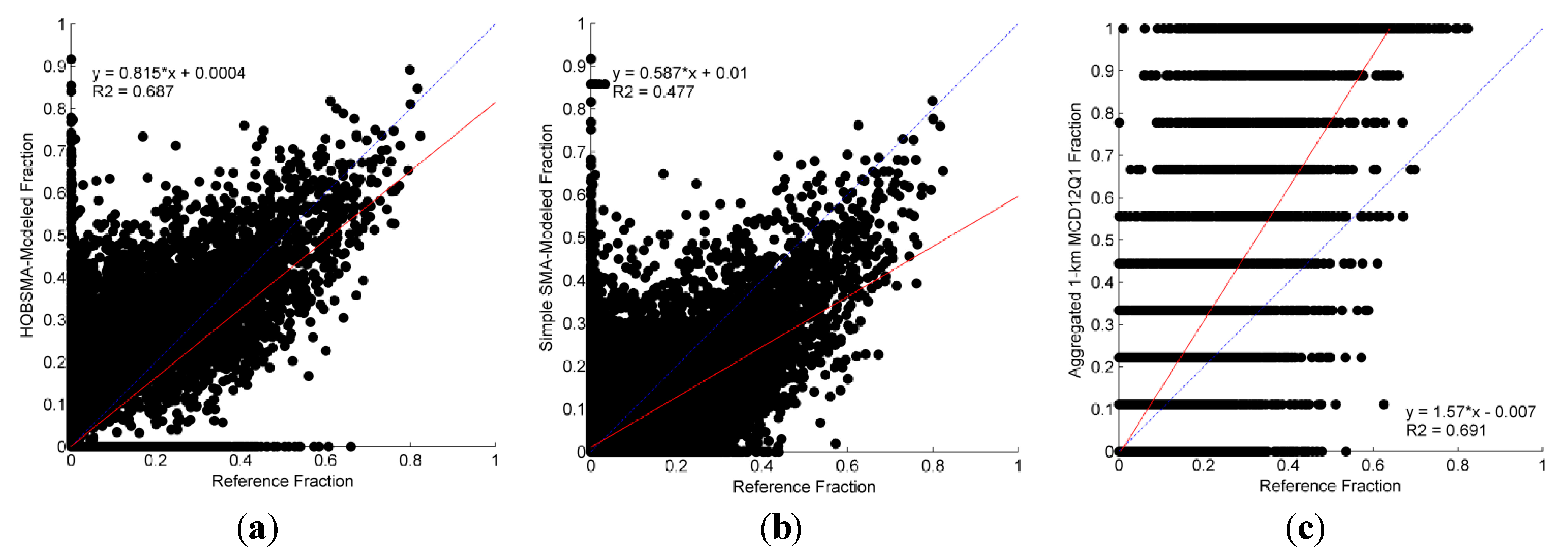
A comparison between scatterplots in Figure 6a,b indicates that HOBSMA has much better regression parameters of the scatter plot than the simple SMA: a much higher slope (0.815 vs. 0.587), an intercept closer to 0 (−0.0004 vs. 0.01), and a much higher R-squared value (0.687 vs. 0.477).

(3)

Quantitative accuracy metrics in Table 1 further confirms that HOBSMA significantly outperforms simple SMA with much better accuracy indicators in all three scenarios of urban development levels, which is consistent with the visual comparisons as mentioned in the first key point.

Both visual examinations and quantitative comparisons suggest that HOBSMA has a more satisfactory performance than simple SMA. It is probably because both between- and within-class endmember variations were accommodated appropriately by using HOBSMA.

4.2.2. Comparisons with the Aggregated MODIS Product

Another comparison was conducted between the HOBSMA-modeled abundance map and the aggregated 1-km MCD12Q1 data. Figure 5f shows that, although its overall pattern is consistent with the reference NLCD map, the Twin Cities area is apparently associated with much brighter pixels when compared to Figure 5g. This suggests that the aggregated MCD12Q1 product is likely to greatly overestimate the impervious surface fraction in urban areas. This is supported by the scatterplot in Figure 6c. Apparent overestimations can be found in most pixels, with a very high slope (1.57) and a negative intercept (−0.007) of the regression line. Quantitative analysis in Table 1 further confirms these observations: the substantial overestimation within urban areas result in three very large error indicators (41.46% for RMSE, 36.94% for MAE, and 29.10% for SE), all of which are much greater than the metrics of HOBSMA. Underestimation can be noticed in less developed areas as well, of which the accuracy metrics are also slightly poorer than those of HOBSMA. Both visual comparisons and assessment indices confirm the better representation of urban land cover abundance generated by HOBSMA. Some interesting observations involved other land covers in areas of interest will be detailed in the discussion section below.

5. Discussions

In an attempt to address the endmember variability issue with the 1-km resolution imagery, the proposed HOBSMA made full use of spatial, spectral, and temporal information.

5.1. Spatial Constraints by HOBSMA for Deriving Local Endmembers and Regional Libraries

An important feature of HOBSMA is the integration of contextual information from two hierarchical levels as spatial constraints into MESMA to account for endmember variability. While OBIA techniques are designed for high spatial resolution imagery, they may also be used with low resolution imagery as the preprocessing of subpixel analysis for large-scale mapping. By extending Tobler’s first law of geography [51] in remote sensing, spatial clusters of similar land covers result in spectral dependence, even at the km-level scale. In this research, OBIA is extended as an inherent tool in the preprocessing step for spectral unmixing at the km scale. Two aspects of its use can be summarized. First, at the lower level, contextual information of child patches is served as a spatial constraint for region-specific endmember generation. Space was partitioned into a number of relatively homogeneous subdivisions (i.e., child patches) by OBIA, in which extrapolated regional-specific endmembers can effectively capture the spectral feature of the dominant land cover (as shown in Figure 4). Second, at the higher level, contextual information of parent patches is employed to spatially constrain the construction of different regional spectral libraries. This processing is a logical extension of the “regionally specific library” first proposed in the pioneering work of MESMA [21]. In HOBSMA, as closer child patches tend to have similar land compositions, regional libraries are constructed by merging adjacent small child patches into their respective baseline child patch in the same parent region, by which the same endmembers can be shared based on their adjacency for unmixing. Contextual information is further adopted for the construction of a larger dynamic regional library when the RMSE criterion is not met (i.e., no representative endmember is found in the current single regional library). Theoretically, a regional library is a subset of the global library, or more explicitly, a space-dependent subset. The computational efficiency therefore can be greatly increased in the iterative unmixing with such a small subset than a global library [52]. Further, by using similarly portable spatial constraints from one level to the next level, HOBSMA is also a logical extension of hierarchical MESMA [61], two significant differences can summarized though. First, the purpose and usage of spatial constraints varies. The constraints in hierarchical MESMA are used to determine detailed material classes for further unmixing [61], while the constraints in HOBSMA are adopted to constrain the spatial extent of image regions for endmembers extrapolation and regional library construction. Second, spatial constraints were derived by using different classifications: pixel-based classification for hierarchical MESMA, while object-based classification for HOBSMA.

5.2. Endmembers at the km Scale: within-Class Synthetic Endmembers and Endmember Variability

Without a doubt, the best option to select endmembers is the direct extraction of image pixels or portable use of field and laboratory spectra. However, this is almost impossible at the km-level scale, particularly for urban impervious surfaces. With low resolution imagery, endmember signatures were alternatively derived through LSS-based extrapolation followed by the endmember refinement. Essentially, as an approximation of real spectra, such extrapolated endmember signatures may not represent homogeneous spectra of any specific material or vegetation type belonging to one category. Instead, these signatures are more likely to be a spectral generalization. For example, the extrapolated spectra of urban impervious surface endmember at a coarse resolution is likely to be a mixed signature of different types of manmade impervious materials, such as a mixture of asphalt, concrete, tiles, and metal, with different colors, conditions, and age. Another example could be the mixture of tree leaves, non-photosynthetic vegetation and shade in the forest areas. These general endmembers (referred to within-class synthetic (WCS) endmembers), however, could still characterize spectral features of different major land covers at the km-level scale with low resolution imagery. The idea of WCS endmember can also be regarded as an extension of virtual endmember (VE) [62,63]. The VE concept refers to a mixture of endmembers of different land cover types (e.g., tree and soil). In contrast to different classes, the WCS endmember used in this research is a synthesis of subclasses of the same endmember category (e.g., a mixture of subclasses of different impervious surfaces) [63]. Moreover, when a number of WCS endmembers were extrapolated within different spatially constraints (referred to spatially constrained WCS endmembers), the spatially constrained WCS endmembers have demonstrated their ability to incorporate endmember variability into linear spectral unmixing as illustrated in this study. The concept of spatially constrained WCS endmembers has been similarly implied and employed in another previous work using Landsat ETM+ imagery at the 30 m resolution [36]. In that work, pixel-specific synthetic endmember signatures were generated as the distance weighted spectra of those automatically extracted endmembers within its neighborhood, which essentially were WCS endmembers. Despite different spatial resolutions, two potential advantages with spatially constrained WCS endmembers can be summarized, including the derivation of regionally specific endmembers, and the increasing possibility of larger between-class variations. While adequate abundance results can be achieved in both studies, additional research on spatially constrained WCS endmembers is still necessary.

Some interesting findings about endmember variability were also observed. First, the spectral contrast between subpixel urban impervious surface and water seems to be increased at the km scale. Generally, pure water pixels and water-contaminated pixels are masked out in the pre- or post-processing step through unsupervised classification or ancillary data to avoid the overestimation of dark impervious surface [7,64]. In contrast, with the use of WCS endmembers at the 1-km resolution, urban impervious surfaces have slightly higher signatures due to the mixture with high albedo materials in urbanized areas, such as concrete and metal. When WCS endmembers are employed in iterative linear unmixing with low-resolution imagery, water-contaminated pixels thus favor a model combination with water endmembers over models with impervious surface endmembers. As such, both land cover abundances could be readily distinguished. This reason can also explain the improved discrimination between urban impervious surface and bare soil with WCS endmembers in HOBSMA, but continuing future studies are still warranted to validate these findings. In addition to the increased between-class variability, the within-class variability of urban impervious surface and water seems to be suppressed by using WCS endmember. As shown in Figure 4, the variations of impervious surface and water are not as large as those of natural vegetation and cropland. These observed associations between endmember variability and spatial scale could be further used in future studies to improve large-scale land cover abundance mapping.

5.3. Temporal Endmember Signatures at the km Scale

Another effort to address endmember variability is the extrapolation of time-series endmember signatures, which represents the phenological variations between different endmembers. Although time-series endmembers have been used in various studies at resolutions of 250 m and 500 m [7,24,65,66], temporal endmember profiles have rarely been derived at the km-level scale also because of the absence of image endmembers. Containing phenological variations (particularly during the maturity period for crops in planted lands), the extrapolated temporal-spectral endmember signatures lessen the confusion between urban impervious surface and bare soil in cropland/planted lands. The effectiveness of phenological features in this research was confirmed to ease the confusion between urban impervious surface and bare soil in cropland, but was further extended from finer resolutions to the km-level scale.

5.4. The Performance in Two Areas of Interests

Urban fringe areas and small settlements have been identified as areas that are prone to mapping error with coarse resolution imagery [11]. Therefore, two such areas of interests in Minnesota were selected to further visually examine the performance of HOBSMA for estimating fractional land covers, particularly to examine the potential confusions with bare soil, as well as with water. The first example is the urban fringe area of the Twin Cities (see Figure 7). Figure 7a,c are the reference maps: the 2006 NLCD percent impervious surface and land cover classification data. Figure 7e shows the MCD12Q1 product, and Figure 7b,d and f display the HOBSMA modeled subpixel land cover abundance maps at 1-km resolution. All three resultant land cover subpixel maps are in good agreement with the other two NLCD reference maps. For example, the pixels with a high fraction of impervious surface (shown in bright grey) in Figure 7b correspond to the high-density developed pixels (shown in purple) in Figure 7a, while the pixels with a medium fraction (shown in dark grey) are in accordance with the medium-density developed pixels (shown in pink). It is also found that the patterns of the abundance maps of cropland and water are similar to their counterparts in the NLCD land cover map. For instance, bright gray pixels in the east and southeast in Figure 7d correspond to croplands in those yellow and brown pixels of cropland in Figure 7c, while bright gray pixels in the southeast in Figure 7f are consistent with the larger lakes and wider river channel in Figure 7c. Comparatively, although an overall pattern of MCD12Q1 is comparable with that of the NLCD land cover map, it can be discerned that all urban pixels in the Twin Cities are labeled with no differences (when comparing to all abundance maps with land cover heterogeneity information at the subpixel level), and that some water and cropland in suburban areas are misclassified as urban pixels.

The other scenario is the small suburban settlements in the greater Mankato area. Figure 8a,c display the reference maps of the two NLCD products. Visual comparisons find consistent patterns in all three abundance maps generated by using the proposed algorithm. Figure 8b is a map of the HOBSMA modeled abundance of urban impervious surface. Mankato (the largest town at the center) and its surrounding towns and villages were clearly highlighted, although pixels might be somewhat underestimated with an extremely small fractional impervious surface (e.g., the case of single roads in suburban areas dominated by open lands). In Figure 8d, fractional cropland/planted lands with bare soil are dominated throughout this suburban area, of which the pattern is comparable with that of Figure 8c and consistent with the literature [67]. In Figure 8f, river channels and lakes sparsely located in this area are successfully discerned. Comparatively, apparent underestimations can be easily found in the MODIS land cover classification map in Figure 8e, particularly urban impervious surface pixels (shown in red) in towns and villages as well as water pixels (shown in blue) in various rivers and lakes.

In summary, the comparisons in these two areas of interests confirm that the land cover abundance maps by using HOBSMA are able to provide more accurate information of spatial explicit distribution and quantitative subpixel land cover compositions in both urban fringe areas and small settlements in suburban areas. Further investigations are still needed to improve HOBSMA. First, similar to MESMA, more efforts can be put towards increasing the computational efficiency of HOBSMA automated construction of regional spectral libraries as illustrated in this pilot study. Second, as an inherent nature of OBIA technique, the image segmentation result is still difficult to evaluate [68], and no general consensus has been placed. Although the purpose of this study is not object-based classification and this problem is not very crucial, better segmentation could result in improved computational efficiency for fewer searches for regionally representative endmembers. Third, further research may explore the comparison between the proposed HOBSMA for coarse resolution images and other similar SMA methods that are only designed for medium resolution images [69]. It would be interesting and meaningful when comparing object-based SMAs that are designed at different scales and using distinct image segmentation methods.

Figure 7. Comparisons in the urban fringe area of Twin Cities. The left column: the 30-m products of (a) 2006 NLCD percent impervious surface (black for vegetated areas, pink for low-intensity developed lands, purple for high-intensity developed lands); and The right column: the 1-km fractional abundance maps of (b) urban impervious surfaces; (c) 2006 NLCD land cover classification (red and pink for developed areas, yellow and brown for agricultural lands, blue for water, and green for vegetation); (d) cropland/planted lands; (e) the 500-m MCD12Q1 map using the same color scheme of the NLCD land cover map; and (f) water.

Figure 7. Comparisons in the urban fringe area of Twin Cities. The left column: the 30-m products of (a) 2006 NLCD percent impervious surface (black for vegetated areas, pink for low-intensity developed lands, purple for high-intensity developed lands); and The right column: the 1-km fractional abundance maps of (b) urban impervious surfaces; (c) 2006 NLCD land cover classification (red and pink for developed areas, yellow and brown for agricultural lands, blue for water, and green for vegetation); (d) cropland/planted lands; (e) the 500-m MCD12Q1 map using the same color scheme of the NLCD land cover map; and (f) water.

Figure 8. Comparisons in small towns near Mankato. The left column: the 30-m products of (a) 2006 NLCD percent impervious surface (black for vegetated areas, pink for low-intensity developed lands, purple for high-intensity developed lands); and the right column: the 1-km fractional abundance maps of (b) urban impervious surfaces; (c) 2006 NLCD land cover classification (red and pink for developed areas, yellow and brown for agricultural lands, blue for water, and green for vegetation); (d) cropland/planted lands; (e) the 500-m MCD12Q1 map using the same color scheme of the NLCD land cover map; and (f) water.

Figure 8. Comparisons in small towns near Mankato. The left column: the 30-m products of (a) 2006 NLCD percent impervious surface (black for vegetated areas, pink for low-intensity developed lands, purple for high-intensity developed lands); and the right column: the 1-km fractional abundance maps of (b) urban impervious surfaces; (c) 2006 NLCD land cover classification (red and pink for developed areas, yellow and brown for agricultural lands, blue for water, and green for vegetation); (d) cropland/planted lands; (e) the 500-m MCD12Q1 map using the same color scheme of the NLCD land cover map; and (f) water.

6. Conclusions

Little research has placed emphasis on endmember variability at the 1-km resolution. To address this issue, an HOBSMA unmixing algorithm was proposed through integrating OBIA into SMA for improving accuracy of large-scale subpixel land cover mapping, particularly urban impervious surface. With spatial, spectral and temporal knowledge taken into consideration, three important steps in HOBSMA include: (1) image partitioning at two hierarchical levels; (2) endmember signature extrapolation and regional spectral library construction based on spatial constraints from image segmentation; and (3) MESMA implementation. Results and analyses show that, by using regional spectral libraries with regionally specific endmembers, HOBSMA effectively improves the discriminations between urban impervious surfaces and other land covers with well-known spectral confusions (e.g., bare soil and water), and particularly provides satisfactory representations of urban fringe areas and small settlements. HOBSMA yields promising abundance results at the km-level scale with relatively high precision and small bias, which significantly outperforms the traditional simple mixing model and the aggregated MODIS land cover classification product. HOBSMA can be further employed not only for subpixel mapping of different land covers with coarse resolution imagery, but also for land cover change detection at a large scale. While future studies are warranted to improve the HOBSMA algorithm, this research could benefit studies on regional/global environmental and climate change studies, in which accurate large-scale subpixel land cover abundance is an essential model input.

References

1. Cohen, B. Urban growth in developing countries: A review of current trends and a caution regarding existing forecasts. World Dev. 2004, 32, 23–51. [Google Scholar] [CrossRef]
2. Schueler, T.R. The importance of imperviousness. Watershed Prot. Tech. 1994, 1, 100–111. [Google Scholar]
3. United Nations. Department of Economic and Social Affairs, Population Division. Available online: http://www.un.org/en/development/desa/population/ (accessed on 17 April 2015).
4. Weng, Q. Remote sensing of impervious surfaces in the urban areas: Requirements, methods, and trends. Remote Sens. Environ. 2012, 117, 34–49. [Google Scholar] [CrossRef]
5. Schueler, T.R.; Fraley-McNeal, L.; Cappiella, K. Is impervious cover still important? Review of recent research. J. Hydrol. Eng. 2009, 14, 309–315. [Google Scholar] [CrossRef]
6. Deng, C.; Wu, C. Examining the impacts of urban biophysical compositions on surface urban heat island: A spectral unmixing and thermal mixing approach. Remote Sens. Environ. 2013, 131, 262–274. [Google Scholar] [CrossRef]
7. Yang, F.; Matsushita, B.; Fukushima, T.; Yang, W. Temporal mixture analysis for estimating impervious surface area from multi-temporal MODIS NDVI data in Japan. ISPRS J. Photogram. Remote Sens. 2012, 72, 90–98. [Google Scholar] [CrossRef] [Green Version]
8. Deng, C.; Wu, C. The use of single-date MODIS imagery for estimating large-scale urban impervious surface fraction with spectral mixture analysis and machine learning techniques. ISPRS J. Photogramm. Remote Sens. 2013, 86, 100–110. [Google Scholar] [CrossRef]
9. Seto, K.C. Global urban issues—A primer. In Global Mapping of Human Settlements: Experiences, Data Sets, and Prospects; CRC Press: Boca Raton, FL, USA, 2009. [Google Scholar]
10. Schneider, A.; Friedl, M.A.; McIver, D.K.; Woodcock, C.E. Mapping urban areas by fusing multiple sources of coarse resolution remotely sensed data. Photogramm. Eng. Remote Sens. 2003, 69, 1377–1386. [Google Scholar] [CrossRef]
11. Schneider, A.; Friedl, M.A.; Potere, D. Mapping global urban areas using MODIS 500-m data: New methods and datasets based on “urban ecoregions”. Remote Sens. Environ. 2010, 114, 1733–1746. [Google Scholar] [CrossRef]
12. Lu, D.; Tian, H.; Zhou, G.; Ge, H. Regional mapping of human settlements in southeastern China with multisensor remotely sensed data. Remote Sens. Environ. 2008, 112, 3668–3679. [Google Scholar] [CrossRef]
13. Lu, D.; Batistellab, M.; Morana, E.; Hetricka, S.; Alves, D.; Brondizioa, E. Fractional forest cover mapping in the Brazilian Amazon with a combination of MODIS and TM images. Int. J. Remote Sens. 2011, 32, 7131–7149. [Google Scholar] [CrossRef]
14. Friedl, M.A.; Sulla-Menashe, D.; Tan, B.; Schneider, A.; Ramankutty, N.; Sibley, A.; Huang, X. MODIS Collection 5 global land cover: Algorithm refinements and characterization of new datasets. Remote Sens. Environ. 2010, 114, 168–182. [Google Scholar] [CrossRef]
15. Bartholomé, E.; Belward, A.S. GLC2000: A new approach to global land cover mapping from Earth observation data. Int. J. Remote Sens. 2005, 26, 1959–1977. [Google Scholar] [CrossRef]
16. Global Rural-Urban Mapping Project (GRUMP). Available online: http://sedac.ciesin.columbia.edu/data/collection/grump-v1 (accessed on 17 April 2015).
17. Potere, D.; Schneider, A.; Angel, S.; Civco, D.L. Mapping urban areas on a global scale: Which of the eight maps now available is more accurate? Int. J. Remote Sens. 2009, 30, 6531–6558. [Google Scholar] [CrossRef]
18. Hansen, M.C.; DeFries, R.S.; Townshend, J.R.G.; Sohlberg, R. Global land cover classification at 1 km spatial resolution using a classification tree approach. Int. J. Remote Sens. 2000, 21, 1331–1364. [Google Scholar] [CrossRef]
19. Hansen, M.C.; DeFries, R.S.; Townshend, J.R.G.; Sohlberg, R.; Dimiceli, C.; Carroll, M. Towards an operational MODIS continuous field of percent tree cover algorithm: Examples using AVHRR and MODIS data. Remote Sens. Environ. 2002, 83, 304–320. [Google Scholar] [CrossRef]
20. Tuanmu, M.N.; Jetz, W. A global 1-km consensus land-cover product for biodiversity and ecosystem modelling. Glob. Ecol. Biogeogr. 2014, 23, 1031–1045. [Google Scholar] [CrossRef]
21. Roberts, D.A.; Gardner, M.; Church, R.; Ustin, S.; Scheer, G.; Green, R.O. Mapping chaparral in the Santa Monica Mountains using multiple endmember spectral mixture models. Remote Sens. Environ. 1998, 65, 267–279. [Google Scholar] [CrossRef]
22. Bateson, C.A.; Asner, G.P.; Wessman, C.A. Endmember bundles: A new approach to incorporating endmember variability into spectral mixture analysis. IEEE Trans. Geosci. Remote Sens. 2000, 38, 1083–1094. [Google Scholar] [CrossRef]
23. Gamba, P.; Herold, M. Global Mapping of Human Settlements: Experiences, Datasets, and Prospects; CRC Press: Boca Raton, FL, USA, 2009. [Google Scholar]
24. Shao, Y.; Lunetta, R.S. Subpixel mapping of tree canopy, impervious surfaces, and cropland in the Laurentian Great Lakes Basin using MODIS time-series data. IEEE J. Sel. Top. Appl. Earth Obs. Remote Sens. 2011, 4, 336–347. [Google Scholar] [CrossRef]
25. Adams, J.B.; Smith, M.O.; Johnson, P.E. Spectral mixture modeling: A new analysis of rock and soil types at the Viking Lander 1 site. J. Geophys. Res. 1986, 91, 8098–8112. [Google Scholar] [CrossRef]
26. Adams, J.B.; Sabol, D.E.; Kapos, V.; Almeida Filho, R.; Roberts, D.A.; Smith, M.O.; Gillespie, A.R. Classification of multispectral images based on fractions of endmembers: Application to land-cover change in the Brazilian Amazon. Remote Sens. Environ. 1995, 52, 137–154. [Google Scholar] [CrossRef]
27. Smith, M.O.; Ustin, S.L.; Adams, J.B.; Gillespie, A.R. Vegetation in deserts: I. A regional measure of abundance from multispectral images. Remote Sens. Environ. 1990, 31, 1–26. [Google Scholar] [CrossRef]
28. Ballantine, J.A.C.; Okin, G.S.; Prentiss, D.E.; Roberts, D.A. Mapping north African landforms using continental scale un-mixing of MODIS imagery. Remote Sens. Environ. 2005, 97, 470–483. [Google Scholar] [CrossRef]
29. Meyer, T.; Okin, G.S. Evaluation of spectral unmixing techniques using MODIS in a structurally complex savanna environment for retrieval of green vegetation, nonphotosynthetic vegetation, and soil fractional cover. Remote Sens. Environ. 2015, 161, 122–130. [Google Scholar] [CrossRef]
30. Eckmann, T.C.; Roberts, D.A.; Still, C.J. Using multiple endmember spectral mixture analysis to retrieve subpixel fire properties from MODIS. Remote Sens. Environ. 2008, 112, 3773–3783. [Google Scholar] [CrossRef]
31. DeFries, R.S.; Townshend, J.R.G.; Hansen, M.C. Continuous fields of vegetation characteristics at the global scale at 1-km resolution. J. Geophys. Res. Atmos. 1999, 104, 16911–16923. [Google Scholar] [CrossRef]
32. Shoshany, M.; Svoray, T. Multidate adaptive unmixing and its application to analysis of ecosystem transitions along a climatic gradient. Remote Sens. Environ. 2002, 82, 5–20. [Google Scholar] [CrossRef]
33. Pignatti, S.; Cavalli, R.M.; Cuomo, V.; Fusilli, L.; Pascucci, S.; Poscolieri, M.; Santini, F. Evaluating hyperion capability for land cover mapping in a fragmented ecosystem: Pollino National Park, Italy. Remote Sens. Environ. 2009, 113, 622–634. [Google Scholar] [CrossRef]
34. Somers, B.; Asner, G.P.; Tits, L.; Coppin, P. Endmember variability in spectral mixture analysis: A review. Remote Sens. Environ. 2011, 115, 1603–1616. [Google Scholar] [CrossRef]
35. Zhang, J.; Rivard, B.; Sanchez-Azofeifa, A.; Castro-Esau, K. Intra- and inter-class spectral variability of tropical tree species at La Selva, Costa Rica: Implications for species identification using HYDICE imagery. Remote Sens. Environ. 2006, 105, 129–141. [Google Scholar] [CrossRef]
36. Deng, C.; Wu, C. A spatially adaptive spectral mixture analysis method for mapping subpixel urban impervious surface distribution. Remote Sens. Environ. 2013, 133, 62–70. [Google Scholar] [CrossRef]
37. Somers, B.; Zortea, M.; Plaza, A.; Asner, G.P. Automated extraction of image-based endmember bundles for improved spectral unmixing. Sel. Top. Appl. Earth Obs. Remote Sens. IEEE J. 2012, 5, 396–408. [Google Scholar] [CrossRef]
38. Asner, G.P.; Lobell, D.B. A biogeophysical approach for automated SWIR unmixing of soils and vegetation. Remote Sens. Environ. 2000, 74, 99–112. [Google Scholar] [CrossRef]
39. Okin, G.S.; Clarke, K.; Lewis, M. Comparison of methods for estimation of absolute vegetation and soil fractional cover using MODIS normalized BRDF-adjusted reflectance data. Remote Sens. Environ. 2008, 130, 266–279. [Google Scholar] [CrossRef]
40. Fry, J.; Xian, G.; Jin, S.; Dewitz, J.; Homer, C.; Yang, L.; Barnes, C.; Herold, N.; Wickham, J. Completion of the 2006 national land cover database for the conterminous United States. Photogramm. Eng. Remote Sens. 2011, 77, 858–864. [Google Scholar]
41. Van der Meer, F.D.; Jia, X. Collinearity and orthogonality of endmembers in linear spectral unmixing. Int. J. Appl. Earth Obs. Geoinf. 2012, 18, 491–503. [Google Scholar] [CrossRef]
42. Loveland, T.R.; Belward, A.S. The IGBP-DIS global 1km land cover data set, DISCover: First results. Int. J. Remote Sens. 1997, 18, 3289–3295. [Google Scholar] [CrossRef]
43. Loveland, T.R.; Zhu, Z.; Ohlen, D.O.; Brown, J.F.; Reed, B.C.; Yang, L. An analysis of the IGBP global land-cover characterization process. Photogramm. Eng. Remote Sens. 1999, 65, 1021–1032. [Google Scholar]
44. Strahler, A.H.; Muller, J.P.; Lucht, W.; Schaaf, C.B.; Tsang, T.; Gao, F.; Barnsley, M.J. MODIS BRDF/Albedo Product: Algorithm Theoretical Basis Document Version 5.0. Available online: http://citeseerx.ist.psu.edu/viewdoc/download?doi=10.1.1.124.3&rep=rep1&type=pdf (accessed on 17 April 2015).
45. Jensen, J.R. Introductory Digital Image Processing: A Remote Sensing Perspective; Prentice-Hall Inc.: Upper Saddle River, NJ, USA, 2004. [Google Scholar]
46. Ridd, M.K. Exploring a VIS (vegetation-impervious surface-soil) model for urban ecosystem analysis through remote sensing: Comparative anatomy for cities. Int. J. Remote Sens. 1995, 16, 2165–2185. [Google Scholar] [CrossRef]
47. Nock, R.; Nielsen, F. Statistical region merging. IEEE Trans. Pattern Anal. Mach. Intell. 2004, 26, 1452–1458. [Google Scholar] [CrossRef] [PubMed]
48. Huang, Z.; Zhang, J.; Li, X.; Zhang, H. Remote sensing image segmentation based on dynamic statistical region merging. Opt. Int. J. Light Electron. Opt. 2014, 125, 870–875. [Google Scholar] [CrossRef]
49. Li, H.; Gu, H.; Han, Y.; Yang, J. An efficient multiscale SRMMHR (Statistical Region Merging and Minimum Heterogeneity Rule) segmentation method for high-resolution remote sensing imagery. IEEE J. Sel. Top. Appl. Earth Obs. Remote Sens. 2009, 2, 67–73. [Google Scholar] [CrossRef]
50. Lang, F.; Yang, J.; Li, D.; Zhao, L.; Shi, L. Polarimetric SAR image segmentation using statistical region merging. IEEE Trans. Geosci. Remote Sens. Lett. 2014, 11, 509–513. [Google Scholar] [CrossRef]
51. Tobler, W. A computer movie simulating urban growth in the Detroit region. Econ. Geogr. 1970, 46, 234–240. [Google Scholar] [CrossRef]
52. Wu, C.; Deng, C.; Jia, X. Spatial-constrained multiple endmember spectral mixture analysis for quantifying sub-pixel urban impervious surfaces. IEEE J. Sel. Top. Appl. Earth Obs. Remote Sens. 2014, 7, 1976–1984. [Google Scholar]
53. Soille, P. Morphological Image Analysis: Principles and Applications; Springer-Verlag Inc.: New York, NY, USA, 2003. [Google Scholar]
54. Pu, R.; Xu, B.; Gong, P. Oakwood crown closure estimation by unmixing Landsat TM data. Int. J. Remote Sens. 2003, 24, 4422–4445. [Google Scholar] [CrossRef]
55. Rouse, J.W., Jr; Haas, R.H.; Schell, J.A.; Deering, D.W. Monitoring vegetation systems in the Great Plains with ERTS. NASA Spec. Publ. 1974, 351, 309. [Google Scholar]
56. Zhu, Z.; Woodcock, C.E. Object-based cloud and cloud shadow detection in Landsat imagery. Remote Sens. Environ. 2012, 118, 83–94. [Google Scholar] [CrossRef]
57. Vermote, E.; Saleous, N. LEDAPS Surface Reflectance Product Description, Version 2.0; University of Maryland: College Park, MD, USA, 2007. [Google Scholar]
58. Powell, R.; Roberts, D.A.; Hess, L.; Dennison, P. Sub-pixel mapping of urban land cover using multiple endmember spectral mixture analysis: Manaus, Brazil. Remote Sens. Environ. 2007, 106, 253–267. [Google Scholar] [CrossRef]
59. Demarchi, L.; Canters, F.; Chan, J.C.; van de Voorde, T. Multiple endmember unmixing of CHRIS/Proba Imagery for mapping impervious surfaces in urban and suburban environments. IEEE Trans. Geosci. Remote Sens. 2012, 50, 3409–3424. [Google Scholar] [CrossRef]
60. Roberts, D.A.; Quattrochi, D.A.; Hulley, G.C.; Hook, S.J.; Green, R.O. Synergies between VSWIR and TIR data for the urban environment: An evaluation of the potential for the Hyperspectral Infrared Imager (HyspIRI) Decadal Survey mission. Remote Sens. Environ. 2012, 117, 83–101. [Google Scholar] [CrossRef]
61. Franke, J.; Roberts, D.A.; Halligan, K.; Menz, G. Hierarchical multiple endmember spectral mixture analysis (MESMA) of hyperspectral imagery for urban environments. Remote Sens. Environ. 2009, 113, 1712–1723. [Google Scholar] [CrossRef]
62. Chang, C.I.; Du, Q. Estimation of number of spectrally distinct signal sources in hyperspectral imagery. IEEE Trans. Geosci. Remote Sens. 2004, 42, 608–619. [Google Scholar] [CrossRef]
63. Chen, X.; Chen, J.; Jia, X.; Somers, B.; Wu, J.; Coppin, P. A quantitative analysis of virtual endmembers’ increased impact on the collinearity effect in spectral unmixing. IEEE Trans. Geosci. Remote Sens. 2011, 49, 2945–2956. [Google Scholar] [CrossRef]
64. Wu, C.; Murray, A.T. Estimating impervious surface distribution by spectral mixture analysis. Remote Sens. Environ. 2003, 84, 493–505. [Google Scholar] [CrossRef]
65. Knight, J.; Voth, M. Mapping impervious cover using multi-temporal MODIS NDVI data. IEEE J. Sel. Top. Appl. Earth Obs. Remote Sens. 2011, 4, 303–309. [Google Scholar] [CrossRef]
66. Busetto, L.; Meroni, M.; Colombo, R. Combining medium and coarse spatial resolution satellite data to improve the estimation of subpixel NDVI time series. Remote Sens. Environ. 2008, 112, 118–131. [Google Scholar] [CrossRef]
67. Hart, J.F.; Ziegler, S.S. Landscapes of Minnesota: A Geography; Minnesota Historical Society: St. Paul, MN, USA, 2008. [Google Scholar]
68. Hay, G.J.; Castilla, G. Geographic Object-Based Image Analysis (GEOBIA): A new name for a new discipline. In Object-Based Image Analysis; Springer: Berlin, Germany, 2008; pp. 75–89. [Google Scholar]
69. Zhang, C.; Cooper, H.; Selch, D.; Meng, X.; Qiu, F.; Myint, S.W.; Xie, Z. Mapping urban land cover types using object-based multiple endmember spectral mixture analysis. Remote Sens. Lett. 2014, 5, 521–529. [Google Scholar] [CrossRef]