Article

Detection of Convective Initiation Using Meteorological Imager Onboard Communication, Ocean, and Meteorological Satellite Based on Machine Learning Approaches

1
School of Urban and Environmental Engineering, Ulsan National Institute of Science andTechnology, Ulsan 689-798, South Korea
2
Department of Atmospheric Science & Engineering, Ewha Womans University, Seoul 120-750, South Korea
3
National Meteorological Satellite Center, Korea Meteorological Administration, Jincheon 365-831, South Korea
*
Author to whom correspondence should be addressed.
Those authors contributed equally to this paper.
Remote Sens. 2015, 7(7), 9184-9204; https://doi.org/10.3390/rs70709184
Submission received: 7 April 2015 / Revised: 26 June 2015 / Accepted: 13 July 2015 / Published: 17 July 2015

Abstract

:
As convective clouds in Northeast Asia are accompanied by various hazards related with heavy rainfall and thunderstorms, it is very important to detect convective initiation (CI) in the region in order to mitigate damage by such hazards. In this study, a novel approach for CI detection using images from Meteorological Imager (MI), a payload of the Communication, Ocean, and Meteorological Satellite (COMS), was developed by improving the criteria of the interest fields of Rapidly Developing Cumulus Areas (RDCA) derivation algorithm, an official CI detection algorithm for Multi-functional Transport SATellite-2 (MTSAT-2), based on three machine learning approaches—decision trees (DT), random forest (RF), and support vector machines (SVM). CI was defined as clouds within a 16 × 16 km window with the first detection of lightning occurrence at the center. A total of nine interest fields derived from visible, water vapor, and two thermal infrared images of MI obtained 15–75 min before the lightning occurrence were used as input variables for CI detection. RF produced slightly higher performance (probability of detection (POD) of 75.5% and false alarm rate (FAR) of 46.2%) than DT (POD of 70.7% and FAR of 46.6%) for detection of CI caused by migrating frontal cyclones and unstable atmosphere. SVM resulted in relatively poor performance with very high FAR ~83.3%. The averaged lead times of CI detection based on the DT and RF models were 36.8 and 37.7 min, respectively. This implies that CI over Northeast Asia can be forecasted ~30–45 min in advance using COMS MI data.

Graphical Abstract

1. Introduction

Convective clouds are developed by various weather systems such as meso-scale convective systems, migrating frontal cyclones, and large-scale monsoonal fronts, which often result in heavy rainfall and thunderstorm events [1,2,3,4,5]. Various meteorological hazards, such as lightning, hail, gusty winds, and floods, are closely related to heavy rainfall and thunderstorms accompanied by convective clouds [3,6,7,8,9,10]. These hazards affect infrastructure and result in significant human and socioeconomic loss. Therefore, there is a need to detect convective initiation (CI) prior to heavy rainfall and thunderstorm development in order to minimize damage by such hazards.
Polar orbiting satellites employing infrared channels have been widely used to detect convective clouds since the 1990s [11,12,13,14,15,16,17,18] using brightness temperature (TB) difference depending on cloud types. Setvak and Doswell III [17] used an infrared channel of Advanced Very High Resolution Radiometer (AVHRR) to detect convective storms by assuming that the tops of convective storms are composed of ice cloud particles only and thus they can be characterized as blackbodies. Yuan and Li [18] extracted convective clouds using cloud optical depth and TB obtained from the infrared channels of Moderate Resolution Imaging Spectroradiometer (MODIS), and analyzed physical properties of the clouds. While polar orbiting satellite sensors are very useful to detect convective clouds, they have not been operationally used to detect CI because their temporal resolution of a few days is much longer than the time scale of the development of convective clouds (~hours).
Geostationary satellites are ideal to detect CI because they provide data over large areas with a very high temporal resolution of a few minutes (currently, 15 min is the best). Geostationary Operational Environmental Satellite (GOES) systems and the Spinning Enhanced Visible and Infrared Imager (SEVIRI) onboard Meteorological Second Generation (MSG) meteorological satellites, operated by the National Environmental Satellite Data and Information Service (NESDIS) and European Organization for the Exploitation of Meteorological Satellites (EUMESAT), respectively, are the representative ones. These satellites are equipped with optical sensors that provide visible and infrared imagery at several spectral wavelengths with a spatial resolution of a few kilometers. Many studies have been performed to detect CI using GOES [3,4,19,20,21,22,23,24] and SEVIRI [25,26,27,28,29] data. Based on the fact that TB at spectral channels should vary in time during the course of atmospheric convection [3,24,30], most of the previous studies focused on developing nowcasting algorithms of CI using interest fields of specific spectral channels such as TB, difference of TB at different channels, and the patterns of their temporal variations. SATellite Convection Analysis and Tracking (SATCAST) developed by University of Alabama [3,24] and Rapid Development Thunderstorms (RDT) developed by the Meteo-France and EUMETSAT nowcasting Satellite Application Facility (SAF) [31] are used to detect CI from GOES and SEVIRI data, respectively. The previously developed algorithms were mostly validated for a few regions in North America [3,24] and Europe [26,29], and showed good performances with a probability of detection up to 80% and a false alarm rate of ~60%. However, the performances of such algorithms have not been reported so far over Northeast Asia where convective clouds are prevalent in the East Asian summer monsoon period (Changma in Korea, Mei-Yu in China and Baiu in Japan) and typhoons [32,33]. Convective clouds over the region are frequently accompanied by lightning, strong winds, and localized heavy rainfall events, which result in huge losses of both life and property [32].
Communication, Ocean, and Meteorological Satellite (COMS), the first Korean geostationary satellite, launched on 27 June 2010, is equipped with three payloads: Meteorological Imager (MI), Geostationary Ocean Color Imager, and Ka-band Communication Payload System [34]. The MI was designed to obtain continuous near-real time meteorological products with a pixel size of 1 km using a visible channel and 4 km using four spectral channels such as shortwave infrared, water vapor, and thermal infrared channels. COMS MI scans a local area including the Korean peninsula as the center (2500 × 2500 km) in every 15 min; meanwhile it provides the full disk image of Earth every 3 h. Therefore, COMS MI can be used for nowcasting of CI over Northeast Asia. However, operational CI algorithms for COMS have not been developed yet. As the specification of the spectral bands of COMS MI is similar to that of Multi-functional Transport SATellite-2 (MTSAT-2) Imager operated by Japan, it may be possible to develop CI algorithms for COMS based on the MTSAT-2 CI detection algorithm, i.e., the Rapidly Developing Cumulus Areas (RDCA) derivation algorithm [35]. MTSAT-2 RDCA detects CI over Northeast Asia using several interest fields which were developed by adopting the ideas of the interest fields originally used in the CI detection algorithm for GOES [3]. The RDCA detection algorithm is relatively simple, and uses only one threshold value for each interest field which was determined based only on the case of convective clouds that occurred during the summer season in 2011 [35]. Therefore, MTSAT-2 RDCA might produce inaccurate CI detection products in different times and environments. To apply the interest fields of MTSAT-2 RDCA to COMS MI, new criteria should be used to accurately detect CI caused by various weather systems in Northeast Asia.
In response to these demands, the objectives of this study are to (1) develop a novel approach to CI detection from COMS MI satellite data, (2) evaluate three machine learning models for CI detection in terms of performance and efficiency, and (3) identify key input variables and the optimum lead time for CI detection. COMS MI and lightning observation data used in this study are presented in Section 2. Section 3 describes the methodology for developing CI detection models from COMS MI based on machine learning approaches. Results from the CI detection models and discussion are covered in Section 4. Finally, Section 5 concludes this paper.

2. Data

2.1. COMS MI

COMS MI is the first Korean meteorological sensor to continuously monitor meteorological phenomena and to extract various meteorological parameters with high temporal resolution. COMS MI is composed of five spectral channels: visible (VIS; 0.55–0.8 μm), shortwave infrared (SWIR; 3.5–4.0 μm), water vapor (WV; 6.5–7.0 μm), and thermal infrared (IR1 at 10.3–11.3 μm and IR2 at 11.5–12.5 μm, respectively) (Table 1). The VIS channel scans the surface and atmosphere with 1 km spatial resolution (i.e., a nominal sub-satellite resolution), while the other channels have 4 km resolution. Temporal resolution of COMS MI is 15 min at a standard mode. In the case of extreme weather conditions, COMS MI can collect data at up to eight times an hour (~8 min intervals) [34], from which it is possible to construct an early warning system of meteorological hazards in Northeast Asia. The visible and infrared channels of COMS MI from 2011 to 2014 were used to develop the CI detection models and new criteria of the interest fields in MTSAT-2 RDCA.

2.2. Lightning Data

Since convective clouds are typically accompanied by lightning, lightning observation data can be used as a reliable indicator of CI [36]. Korea Meteorological Administration (KMA) has operated a ground-based Total Lightning Detection System (TLDS) that is composed of 7 IMProved Accuracy from Combined Technology Enhanced Sensitivity and Performance (IMPACT ESP) sensors and 17 Lightning Detection And Ranging (LDAR) II sensors since 2001. IMPACT ESP sensors detect cloud-to-ground discharge while LDAR II sensors observe cloud-to-cloud discharge. The TLDS has a lightning detection accuracy of ~90%, with a location accuracy of 500 m over inland areas and 2 km over the ocean [37]. The TLDS lightning observation data from 2011 to 2014 were used to determine the CI areas from IR1 images of COMS MI.
Table 1. Spectral channel characteristics of COMS MI.
ChannelCenter Wavelength (μm)Bandwidth (μm)Spatial Resolution (km)
VIS0.6750.55 –0.801 × 1
SWIR3.753.5 –4.04 × 4
WV6.756.5 –7.04 × 4
IR110.810.3–11.34 × 4
IR212.011.5–12.54 × 4

3. Methodology

As mentioned, the RDCA detects CI areas from MTSAT-2 images using only one threshold value for each interest field [35]. Such simple criteria of the interest fields might not be sufficient to accurately detect convective clouds driven by various weather systems, which can have diverse values for the interest fields. In this study, the new criteria of the interest fields were assessed to improve the CI detection performance and efficiency using COMS MI data. Binary classification was applied to detect CI from COMS MI data, in which the interest fields of MTSAT-2 RDCA were used as input variables. 
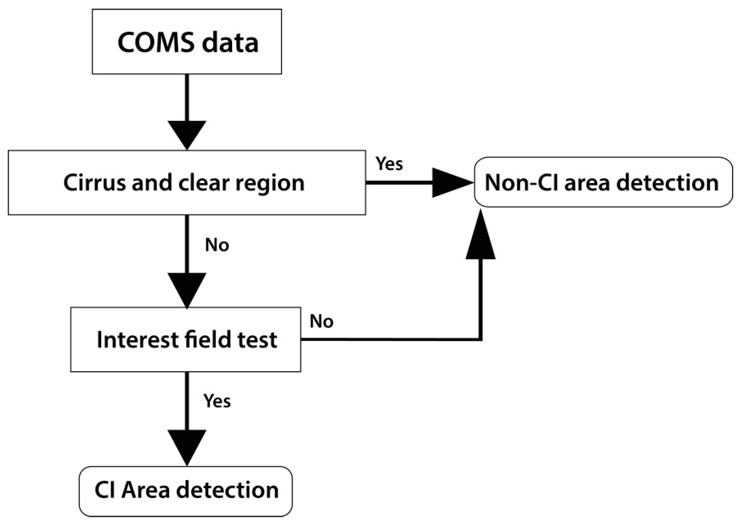
Figure 1 shows the processing flow of the binary classification based on machine learning approaches. This section describes the interest fields of RDCA and three machine learning approaches used for the binary classification of CI and non-CI. The method for collecting samples for classification and validation is also described in this section.
Figure 1. Processing flow of the binary classification of COMS MI images for CI detection based on machine learning approaches.
Remotesensing 07 09184 g001

3.1. Convective Initiation Interest Fields for COMS MI

The interest fields used in RDCA (Table 2) can be used to develop a CI detection model for COMS due to the large similarity of spectral channels between the COMS MI and MTSAT-2 Imager. The VIS channel of MI has 1 km spatial resolution, while the other spectral channels have 4 km resolution. The different spatial resolutions make it difficult to combine the spectral channels. In order to efficiently process data, the COMS MI images were downscaled to 1 km resolution using bilinear interpolation.
Clear sky and thin cloudy areas were removed from MI images using reflectance ( α ) at VIS, TB at IR1, and the difference of TBs between the IR1 and IR2 channels. The term α at VIS varies by solar zenith angle, which produces incorrect interest fields related to the VIS channel. Therefore, α at VIS must be normalized to the solar zenith angle. In this study, α at VIS was normalized by
α ( θ ) = α / cosθ
where α ( θ ) is the normalized reflectance and θ is a solar zenith angle. A criterion of IR1 TB higher than 288.15 K was used to mask areas of clear sky, while criteria of α ( θ ) > 45% and TB difference between IR1 and IR2 < 2 K was used to remove thin clouds and cirrus [35]. These criteria are essential to mask clear sky and thin cloudy areas, but work only in summer season in the absence of snow [35]. Thus, the CI detection models developed in this study can be applied to COMS MI images with such conditions.
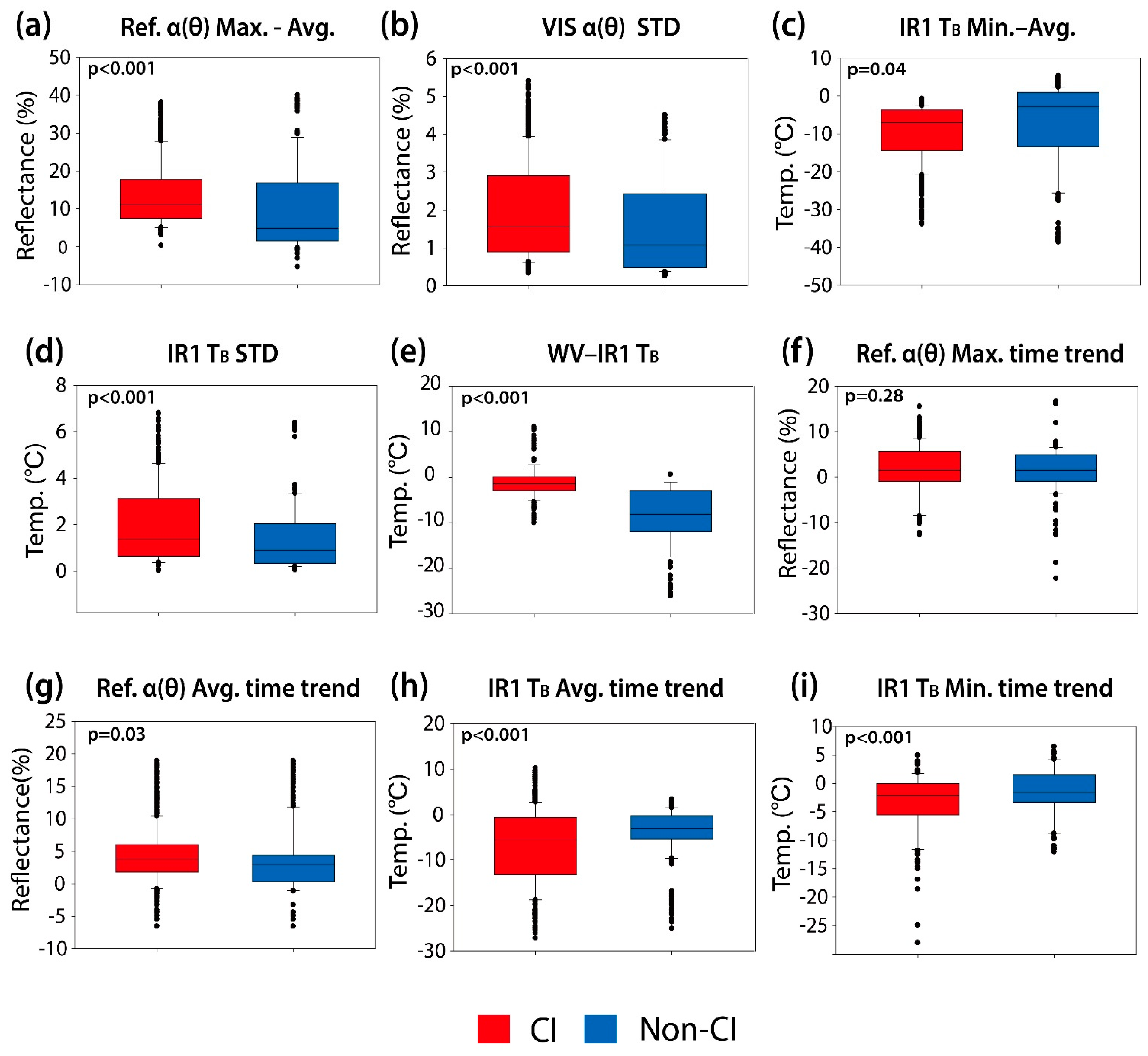
The interest fields in Table 2 are closely related to the growth of clouds. The difference between the maximum and average of VIS α ( θ ) (VIS α ( θ ) Max.–Avg.), the difference between minimum TB and averaged TB at IR1 (IR1 TB Min.–Avg.), and the standard deviations of VIS α ( θ ) and IR1 TB (VIS α ( θ ) STD and IR1 TB STD) represent cloud roughness which is strongly correlated with the growth of clouds [3,35]. The maximum of VIS α ( θ ) and minimum of IR1 TB were calculated using a 7 × 7 pixel window, while the average of VIS α ( θ ) and IR1 TB, and their standard deviations were calculated based on a 21 × 21 pixel window. This follows the methods used in the MTSAT-2 RDCA [35]. VIS α ( θ ) Max.–Avg. and IR1 TB Min.–Avg. represent minute characteristics of clouds developing in the vertical direction in a formative stage [35]. The clouds developed by local strong upward flow show higher reflectance and lower temperature than their surrounding clouds, resulting in increasing VIS α ( θ ) Max.–Avg. and decreasing IR1 TB Min.–Avg. in CI areas [35]. VIS α ( θ ) STD and IR1 TB STD indicate cloud-top asperity, which become apparent as vertically developing clouds [35]. The difference between TBs at WV and IR1 (WV–IR1 TB) is an indicator representing the cloud-top height relative to the tropopause [3,35], which makes possible to estimate the development stage of the clouds. As the surface is typically warmer than the upper troposphere, the value of WV – IR1 TB is usually negative. The values of WV–IR1 TB become negative but near to zero when cumulus clouds evolve into convective ones [3,24,35].
Table 2. Convective initiation interest fields used in this study.
IDInterest FieldsPhysical Characteristics
1VIS α ( θ ) Max.–Avg. differenceDetection of roughness which is observed at rising cloud top
2VIS α ( θ ) STD
3IR1 TB Min.–Avg. difference
4IR1 TB STD
5WV–IR1 TB differenceDetection of water above cloud top
6VIS α ( θ ) Max. time trendPresumption of development level of clouds
7VIS α ( θ ) Avg. time trend
8IR1 TB Avg. time trend
9IR1 TB Min. time trend
The time trends of the maximum and average of VIS α ( θ ) (VIS α ( θ ) Max. time trend and VIS α ( θ ) Avg. time trend, respectively) indicate the growth of clouds over time, while the minimum and average of IR1 TB (IR1 TB Min. time trend and IR1 TB Avg. time trend, respectively) represent the changes in cloud-top height over time [3,35]. To calculate the interest fields, it is necessary to trace the motion of cloud objects. Atmospheric motion vectors have been widely used for tracking clouds [3,24,38]. However, since COMS MI provides atmospheric motion vectors every hour, it is not appropriate to use them for tracing cloud objects every 15 min. Mecikalski et al. [39] proposed a simple cloud object tracking method using two consecutive images obtained over the same area. We adopted the method [39] to trace moving cloud objects from two consecutive IR1 images and then calculated the 15 min difference of the time-dependent interest fields.

3.2. Machine Learning Approaches for CI Detection

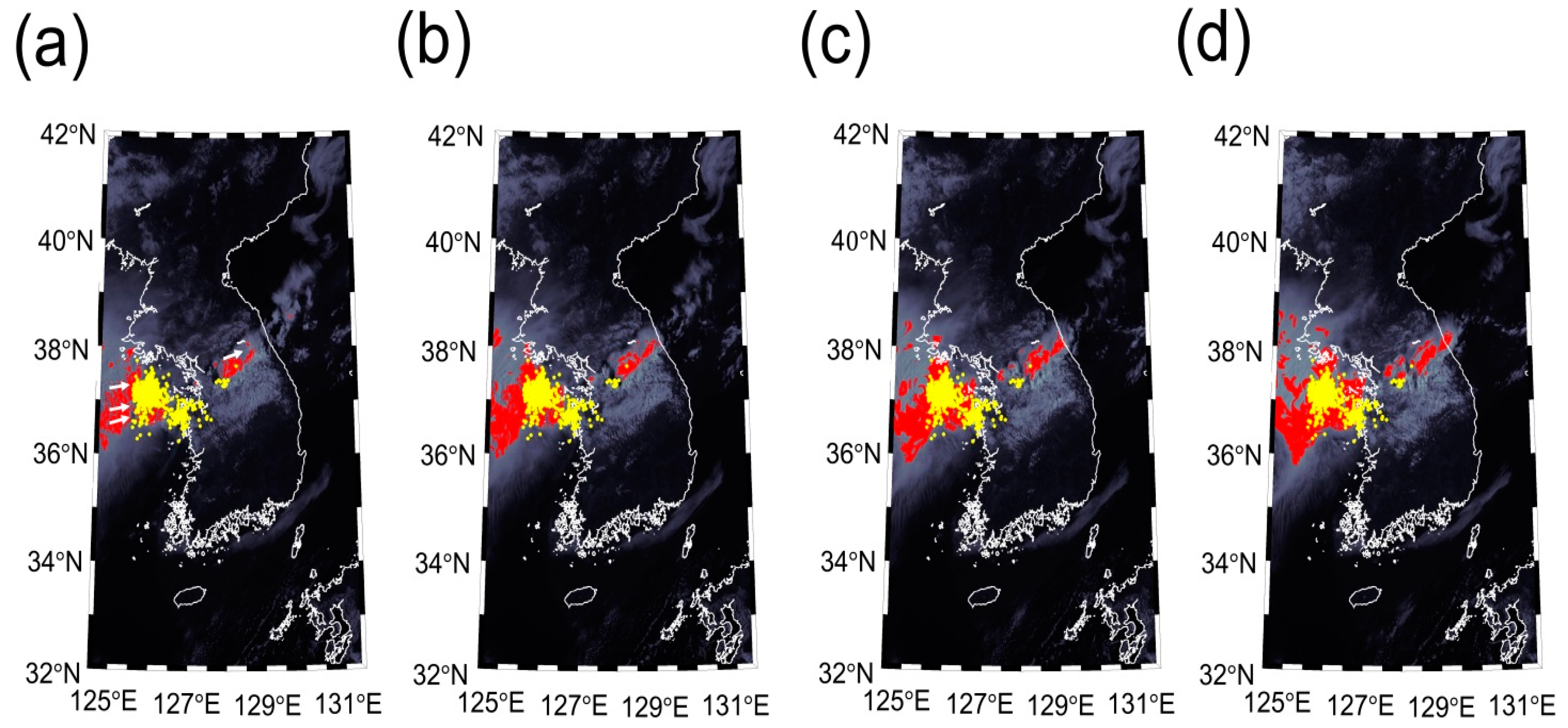
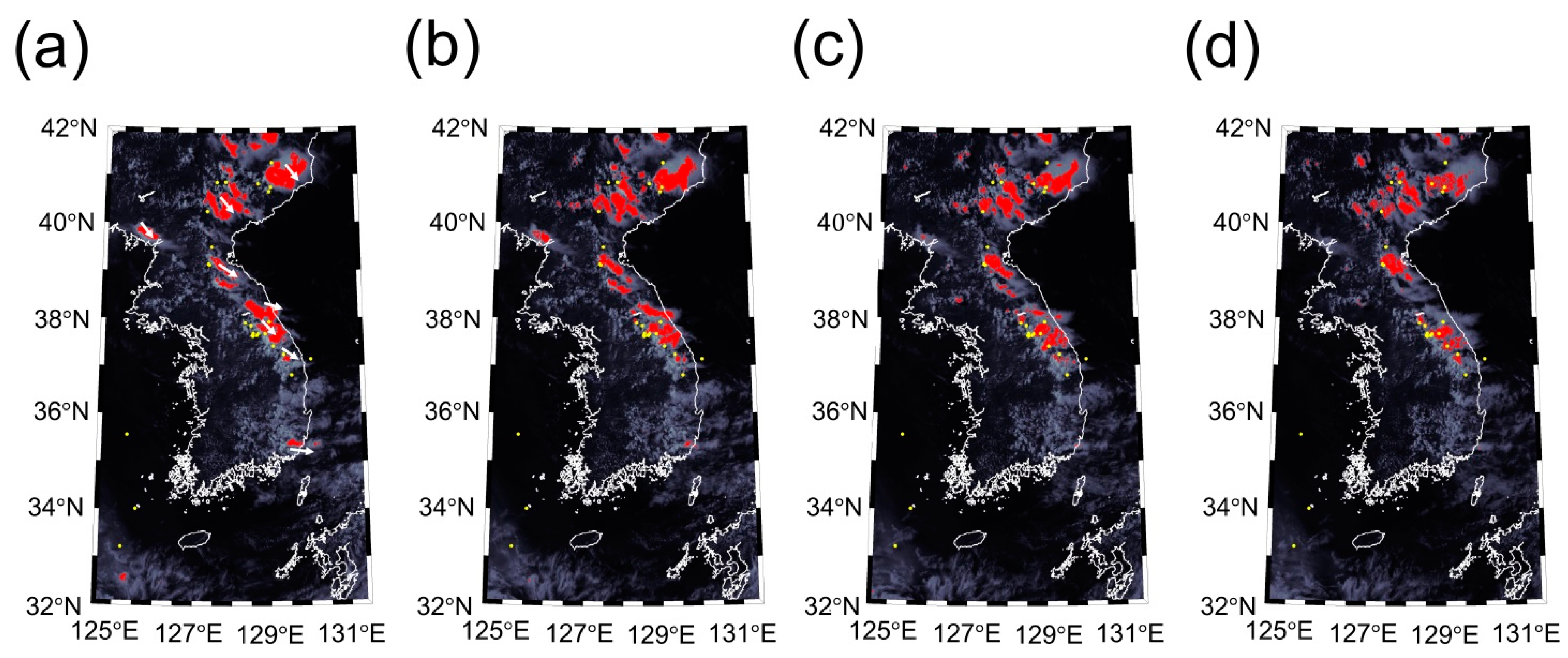
The occurrence of CI is set to a dependent variable for binary classification. For eight cases of CI over South Korea (ID CI1–CI8 in 
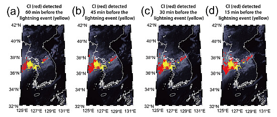
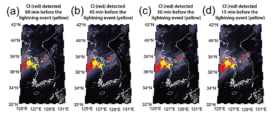
Table 3), the areas of convective clouds (CI areas) were manually delineated from cloudy areas observed in IR1 images of MI by referring to the location and times of lightning. CI areas were defined in this study as clouds within a 16 × 16 km window with the location of the first detection of lightning occurring at the center. The other cloudy areas were considered as non-CI areas. To extract the samples of the interest fields, each CI area was visually tracked from the IR1 images obtained 15–75 min before the image that was acquired at the nearest time of the lightning occurrence, not using the cloud tracking method of Mecikalski et al. [39]. To train and validate machine learning-based classification models, a total of 1072 samples (i.e., pixels) for the interest fields (624 CI and 448 non-CI samples) were selected from the MI images. Eighty percent of the samples for each class (498 samples for CI and 360 samples for non-CI) were used as a training dataset, while the remaining samples (124 samples for CI and 90 samples for non-CI) were used to validate the models.
Table 3. Cases of convective initiations used for development and validation of machine learning based CI detection models.
IDDateTime (hh:mm, UTC)Source of CI
CI13 July 201102:00Frontal cyclone
CI23 August 201101:45
CI323 August 201203:45
CI414 July 201304:15
CI517 May 201204:45Unstable atmosphere
CI69 August 201204:30
CI75 July 201304:00
CI830 June 201407:30
CI93 August 201101:45Frontal cyclone
CI1027 May 201204:45Unstable atmosphere
CI1110 August 201301:00Frontal cyclone
CI1230 June 201407:30Unstable atmosphere
Machine learning, a novel approach used in various remote sensing applications including land use/land cover classification [40,41,42,43,44], vegetation mapping [42,45,46], and change detection [42,47,48], was used for binary classification of CI and non-CI areas from COMS MI data. Three machine learning approaches—decision trees (DT), random forest (RF), and support vector machines (SVM)—were used in this study. To carry out decision tree-based classification, See5 developed by RuleQuest Research, Inc. [49] was used in this study. See5 uses repeated binary splits based on an entropy-related metric to develop a tree. A generated tree can be converted into a series of if-then rules, which makes it easy to analyze the classification results [49,50]. RF builds a set of uncorrelated trees based on Classification and Regression Trees (CART) [51], which is a rule-based decision tree. To overcome the well-known limitation of CART that classification results largely depend on the configuration and quality of training samples [52], the numerous independent trees are grown by randomly selecting a subset of training samples for each tree and a subset of splitting variables at each node of the tree. After the learning process, a final conclusion from the independent decision trees is made by using either a simple majority voting or weighted majority voting strategy. In typical remote sensing applications, See5 and RF use samples extracted from remote sensing data as predictor variables to classify the samples into the target variable (e.g., class attributes in land cover mapping) [
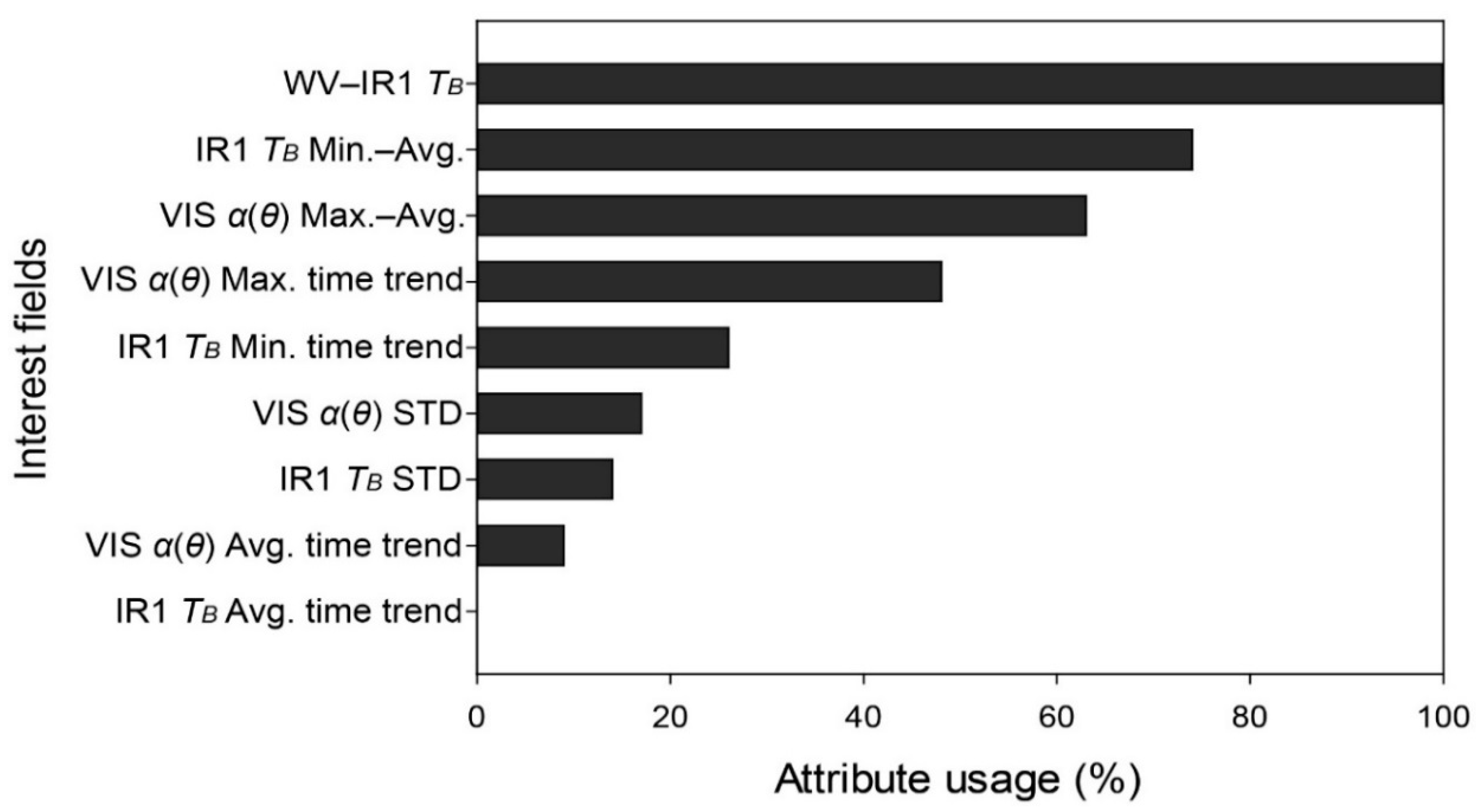
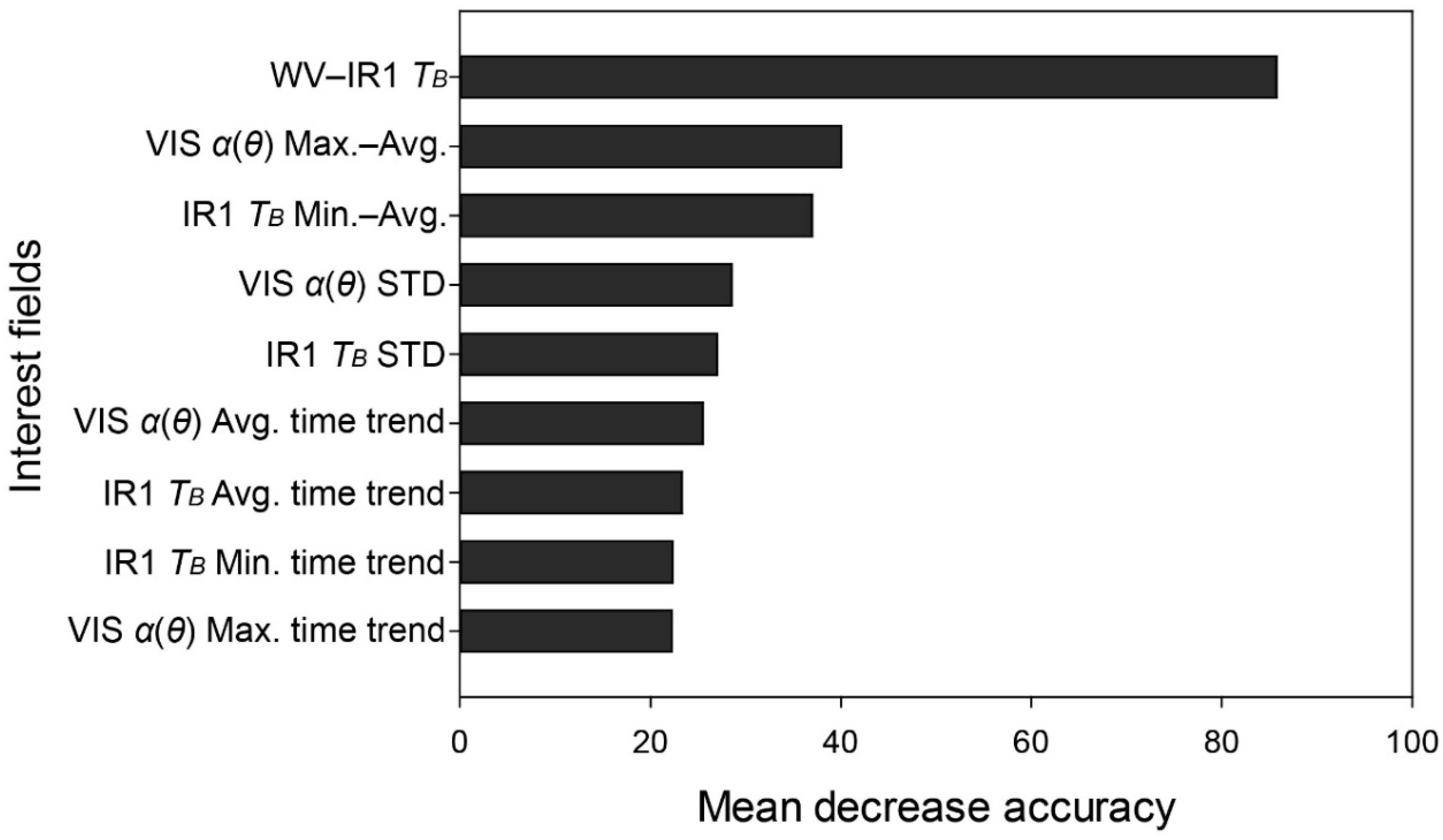
50]. In this study, RF was implemented using an add-on package in R software. See5 and RF in R software produce the information on the relative importance of input variables with attribute usage and mean decrease accuracy, respectively. The attribute usage information shows how the contribution the each variable has to the rules [49], while mean decrease accuracy represents how much accuracy decreases when a variable is randomly permuted [51]. SVM is a supervised learning algorithm, which divides training samples into separate categories by constructing hyperplanes in a multidimensional space, typically a higher dimension than the original data, so the samples can be linearly separable. SVM assumes that the samples in multispectral data can be linearly separated in the input feature space. However, data points of different classes can overlap one another, leading to difficulty in linearly separating the samples. In order to solve such a problem, SVM uses a set of mathematical functions, called kernels, to project data into a higher dimension [53]. Selection of a kernel function and its parameterization are crucial for successful implementation of SVM [54,55]. There are many kernel functions available, and radial basis functions (RBF) have been widely used for remote sensing applications [41,56,57]. In this study, the library for SVM (LIBSVM) software package [58] with a RBF kernel was adopted and the parameters of the kernel were optimized through a grid-search algorithm in LIBSVM.
To evaluate the performance of the three machine learning models, the user’s accuracy, the producer’s accuracy, the overall accuracy, and the kappa coefficient were computed from a confusion matrix of the test dataset which is a specific table for evaluating the performance of a classification result. Overall accuracy can be derived from dividing the number of samples that were correctly classified by the total number of samples. User’s and producer’s accuracies show how well individual classes were classified correctly. The producer’s accuracy (i.e., omission error) refers to the probability that a CI (or a non-CI) area is correctly classified as such, while the user’s accuracy (
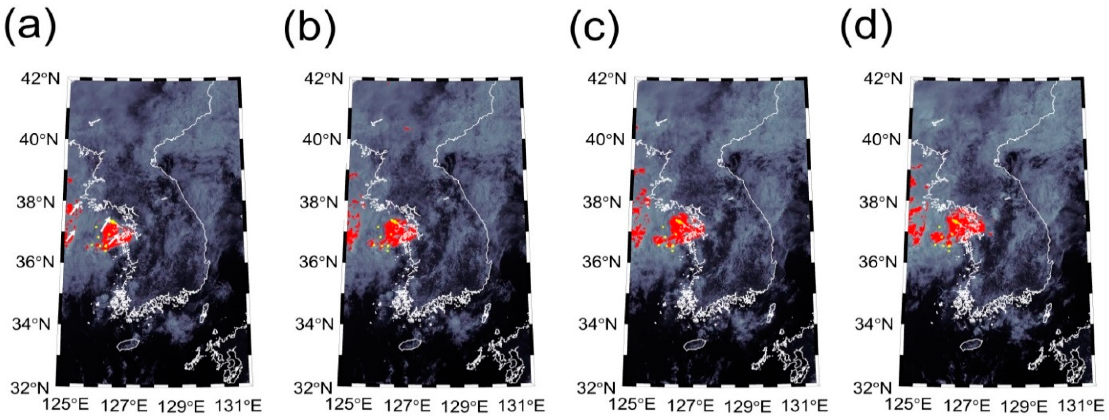
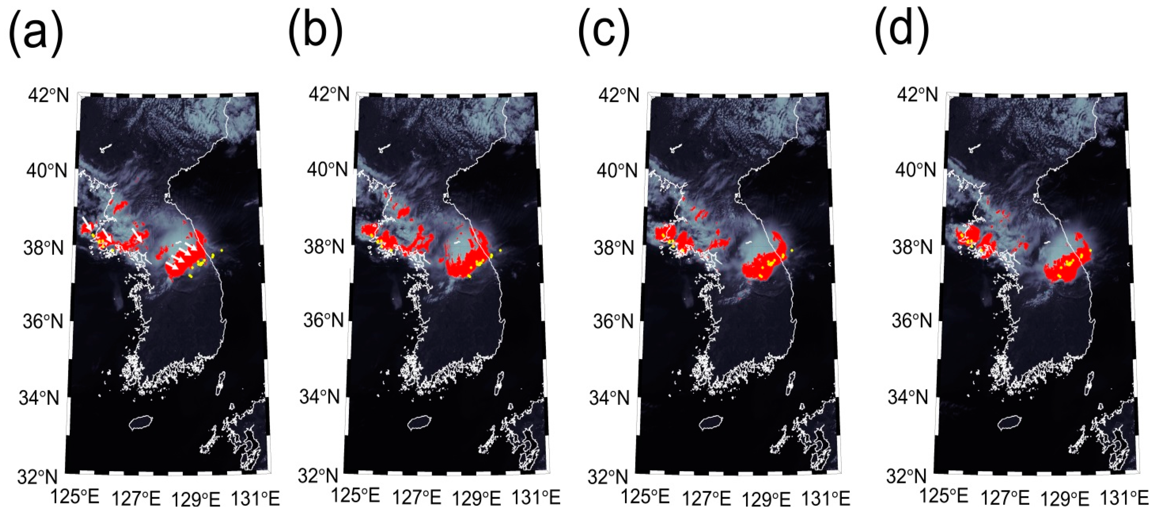
i.e., commission error) refers to the probability that a sample labeled as a CI (or a non-CI) is correctly classified as a certain class. Kappa coefficient, another criterion used for the assessment of classification results, measures the degree of agreement between classification and reference data considering change agreement occurring by chance. Moreover, the developed machine learning models were further validated using the four cases of CI (ID CI9–CI12 in Table 3), from which the probability of detection (POD), false alarm rate (FAR), and accuracy (ACC) were computed as follows [24]:
P O D = H / ( H + M )
F A R = F A / ( F A + H )
A C C = ( H + C N ) / ( H + C N + M + F A )
where H is the number of actual CI objects that were correctly classified as CI (i.e., hits), M is the number of CI objects that were incorrectly marked as non-CI (i.e., misses), FA is the number of non-CI objects that were incorrectly marked as CI (i.e., false alarm), and CN is all the remaining objects that were correctly classified as non-CI (i.e., correct negatives). A cloud object is defined as the lump of connected cloud pixels that resulted from machine learning-based CI detection. As the TLDS lightning data used for validation contain the locations of lightning occurrences only, for each case day, the H, M, FA, and CN were counted from the CI detection results derived from the COMS MI images obtained 15–30, 30–45, 45–60, and 60–75 min before lightning occurrence based on cloud objects. In the MI images obtained at the nearest time of the lightning occurrence, the cloud objects including the position of lightning were regarded as the actual CI. Meanwhile, in the MI images obtained 15–75 min before the image that was acquired at the nearest time of the lightning occurrence, the distances from clouds to the location of lightning occurrence were calculated using hourly atmospheric motion vector products of COMS MI by assuming constant velocity and direction of cloud drift over 1 h. For each case day, atmospheric motion vectors of clouds were averaged to find a typical value of drifting velocity. In the MI images obtained 15–75 min before lightning occurrence, the cloud objects within a given distance from the location of lightning occurrence were regarded as the actual CI. Overall POD, FAR, and ACC were computed for each machine learning model using the H, M, FA, and CN of all case days.
The lead time, the period of time that has elapsed between the CI prediction and the beginning of actual CI, for the four case days was calculated by applying a weighted average depending on H detected from the MI images obtained before lightning occurrence as follows:
H t × n n ( t = 15 , 30 , 45 , 60   min. )
where Ht is the number of H counted from the MI images obtained t minutes before lightning occurrence and n is the number of Ht. The lead time of each machine learning model was determined using Ht and n of all case days.

4. Results

4.1. CI Detection Model Performance

Figure 2 shows box plots of the interest fields using the CI and non-CI samples. Colored boxes represent the interquartile range of the samples, while a line inside the box means median value of the samples. The vertical lines above and below of the box represent 1.5 times interquartile range beyond the lower and upper quartiles, and the points represent the outliers. The p-values in each box plot were derived by t-tests of the CI and non-CI samples of the interest field at the 95% confidence level. Thus, the p-values below 0.05 mean that there is a significant difference between the means of two groups. The values of WV–IR1 TB difference of CI are distinctly higher than those of non-CI (Figure 2e). However, the other interest fields for CI show similar median values or interquartile range to those for non-CI. This means that the use of a fixed threshold value for each interest field, as is widely used in the previously developed CI detection algorithms [3,24,28,35], might not be suitable to detect CI, and suggests the need for multiple adaptive thresholds. Therefore, it is worth developing machine learning-based models that detect CI using multiple rules for the interest fields.
The test dataset was used to produce confusion matrices to assess the performance of the three machine learning models. The DT and RF models showed similar overall accuracies of 98.13% and 99.53%, respectively (Table 4 and Table 5). However, the kappa coefficient of the RF model (99.04%) was slightly higher than that of DT (96.15%). This is possibly because RF uses a superior strategy to categorize samples based on two randomizations. Meanwhile, the SVM model classified the test samples to CI and non-CI perfectly (Table 6) which means that the training and test samples are clearly separated by the optimized hyperplanes.
The relative importance of the input variables (i.e., the interest fields) for CI detection for the DT and RF models is shown in Figure 3 and Figure 4, respectively. WV–IR1 TB, the most distinguishing variable between CI and non-CI as shown in Figure 2e, was identified as the most contributing variable to classify CI and non-CI in both the DT and RF models. The CI and non-CI samples of WV–IR1 TB show the smallest p-value compared to the other interest fields, representing that CI and non-CI have clearly distinct mean values for the interest field, at the 95% confidence level. The TB of WV is less than that of IR1 because of absorption of water vapor [3,35,59,60]. The TB of IR1 is less than that of WV only when cloud tops penetrate in the lower parts of the stratosphere. When the clouds evolve vertically into deep convective clouds, the WV–IR1 TB tends to have negative values but near to zero because of the optical thickness of the clouds, which is distinctive from other cloud types [3,24]. This reveals that WV–IR1 TB is the most important variable for CI detection.
Figure 2. Box plots of the interest fields used for CI detection: (a) VIS α ( θ ) Max.–Avg., (b) VIS α ( θ ) STD, (c) IR1 TB Min.–Avg., (d) IR1 TB STD, (e) WV–IR1 TB, (f) VIS α ( θ ) Max. time trend, (g) VIS α ( θ ) Avg. time trend, (h) IR1 TB Avg. time trend, and (i) IR1 TB Min. time trend.
Remotesensing 07 09184 g002
Table 4. Accuracy assessment results for the DT model using the test dataset.
ReferenceCINon-CISumUser’s Accuracy
Classified as
CI123312697.62%
Non-CI1878898.86%
Sum12490214
Producer’s accuracy99.19%96.67%
Overall accuracy98.13%
Kappa coefficient96.15%
Table 5. Accuracy assessment results for the RF model using the test dataset.
ReferenceCINon-CISumUser’s Accuracy
Classified as
CI1230123100.00%
Non-CI1909198.90%
Sum12490214
Producer’s accuracy99.19%100.00%
Overall accuracy99.53%
Kappa coefficient99.04%
Table 6. Accuracy assessment results for the SVM model using the test dataset
ReferenceCINon-CISumUser’s Accuracy
Classified as
CI1240124100.00%
Non-CI09090100.00%
Sum12490214
Producer’s accuracy100.00%100.00%
Overall accuracy100.00%
Kappa coefficient100.00%
Figure 3. Attribute usage of the DT model.
Remotesensing 07 09184 g003
Figure 4. Mean decrease accuracy calculated using out-of-bag data when a variable was permuted in RF. The greater the decrease in accuracy, the more contributing the variable was.
Remotesensing 07 09184 g004
The next contributing variables for both models were IR1 TB Min.–Avg. and VIS α ( θ ) Max.–Avg. The p-values for IR1 TB Min.–Avg. and VIS α ( θ ) Max.–Avg. were less than 0.05, which also represent that these interest fields significantly contributed to CI detection at the 95% confidence level. IR1 TB Min.–Avg. represents the degree of the vertical development of convective clouds, the value of which increases as clouds develop to convective. The amplitude of VIS α ( θ ) Max.–Avg., representing the cloud roughness, also increases as clouds evolve into convective clouds and induce large reflection at the convective core [3,35,61]. These variables show somewhat similar distribution between CI and non-CI in the boxplots (Figure 2a,c). Nevertheless, they could be used as important variables because the median value of non-CI was not included in the interquartile range of CI for the variables.

4.2. Examination of CI Detection Models for Four Case Days

The machine learning models for CI detection were applied to the four case days (ID CI9–CI12 in Table 3), from which the generated contingency tables and validation statistics are presented in Table 7 and Table 8, respectively. Figure 5, Figure 6, Figure 7 and Figure 8 show the CI detection maps for the four case days generated using the MI images of 15–60 min before lightning occurrence by the RF model. Although the SVM model classified the test samples into CI and non-CI exactly, it produced the lowest performance with an overall FAR of 83.3% (Table 8), compared to the other machine learning models. The FA for the SVM model was much larger than that of the other machine learning models (Table 7), which implies that the hyperplanes separating CI and non-CI could not be valid for various CI cases due to the insufficient number of samples extracted from the training dataset (i.e., CI1–CI8). While the SVM model produced relatively low accuracy from the validation statistics, the two rule-based models, DT and RF, showed good performance for detecting CI (Table 7 and Table 8). Based on the model performance analyzed from the validation statistics, results from the two-rule based models are discussed in the following section.
Table 7. Contingency tables generated from the validation of the DT, RF, and SVM models for the four case days. For each model, the four cells below each case name represent H (top-left cell), M (bottom-left cell), FA (top-right cell), and CN (bottom-right cell).
Case 2011 (Frontal Cyclone)Case 2012 (Unstable Atmosphere)Case 2013 (Frontal Cyclone)Case 2014 (Unstable Atmosphere)
DT2515354251245261
689921862726318503
RF2514363048205274
690021981926716490
SVM3045838139509666192
25892151132087352
Table 8. Validation statistics and averaged lead times from the DT, RF, and SVM models for the four case days.
Case 2011 (Frontal Cyclone)Case 2012 (Unstable Atmosphere)Case 2013 (Frontal Cyclone)Case 2014 (Unstable Atmosphere)Overall
DTPOD80.6%94.6%65.7%74.3%70.7%
FAR37.5%54.5%32.0%54.0%46.6%
ACC97.7%83.3%86.0%87.5%91.2%
Lead time37.8%37.3%36.8%37.8%37.4%
RFPOD80.6%94.7%71.6%76.5%75.5%
FAR35.8%45.4%29.4%58.7%46.2%
ACC97.8%88.0%88.9%85.8%91.7%
Lead time37.8%37.5%37.2%37.5%37.5%
SVMPOD93.8%95.0%79.4%90.4%88.1%
FAR95.2%78.5%65.8%74.4%83.3%
ACC57.5%57.3%70.2%67.7%62.0%
Lead time36.5%36.1%38.4%37.7%37.2%
Figure 5. CI detection maps for the case in 2011 (CI by frontal cyclone) generated from the RF model, overlaid with COMS MI IR1 images obtained (a) 60 min, (b) 45 min, (c) 30 min., and (d) 15 min before the image acquisition at the nearest time of the lightning occurrence. Red objects are the predicted CI and yellow dots represent the location of lightning occurrences. White arrows in (a) represent the movement directions of cloud objects.
Remotesensing 07 09184 g005
Figure 6. CI detection maps for the case in 2012 (CI by unstable atmosphere) generated from the RF model, overlaid with COMS MI IR1 images obtained (a) 60 min, (b) 45 min, (c) 30 min, and (d) 15 min before the image acquisition at the nearest time of the lightning occurrence. Red objects are the predicted CI and yellow dots represent the location of lightning occurrences. White arrows in (a) represent the movement directions of cloud objects.
Remotesensing 07 09184 g006
Figure 7. CI detection maps for the case in 2013 (CI by frontal cyclone) generated from the RF model, overlaid with COMS MI IR1 images obtained (a) 60 min, (b) 45 min, (c) 30 min, and (d) 15 min before the image acquisition at the nearest time of the lightning occurrence. Red objects are the predicted CI and yellow dots represent the location of lightning occurrences. White arrows in (a) represent the movement directions of cloud objects.
Remotesensing 07 09184 g007
Figure 8. CI detection maps for the case in 2014 (CI by unstable atmosphere) generated from the RF model, overlaid with COMS MI IR1 images obtained (a) 60 min, (b) 45 min, (c) 30 min, and (d) 15 min before the image acquisition at the nearest time of the lightning occurrence. Red objects are the predicted CI and yellow dots represent the location of lightning occurrences. White arrows in (a) represent the movement directions of cloud objects.
Remotesensing 07 09184 g008
The RF and DT models yielded similar overall FAR (~46%) and ACC (~91%), while the RF model produced slightly higher overall POD (75.5%) than the DT model (70.7%). Both DT and RF models showed the highest POD for the case in 2012 (94.6% for DT and 94.7% for RF), while they produced the highest ACC for the case in 2011 (97.7% for DT and 97.8% for RF). The CN predicted by all machine learning models was highest for the 2011 case (899 for DT and 900 for RF) due to the wide cloud cover (Figure 5), which contributed to high ACC. Meanwhile, the DT and RF models produced the smallest number of M for the case in 2012 (Table 7 and Figure 6), which resulted in the highest POD compared to the other case days (Table 8).

5. Discussion

The developed machine learning models for CI detection based on COMS MI images showed good performance over the Korea Peninsula with POD higher than 70% and FAR lower than 50% for tracked cloud objects, and could provide a longer lead time than other CI detection algorithms used for other geostationary satellites. However, the machine learning models require the manual tracking of clouds to construct the interest fields because COMS MI has provided hourly atmospheric motion vectors that are not appropriate to track clouds from the MI images acquired every 15 min. Therefore, it is necessary to develop an algorithm for deriving atmospheric motion vectors in a shorter period of time (~15 min) from COMS MI data to forecast CI quickly. As the accuracy of the automation of cloud motion tracking can lead to errors in CI detection, such automation of producing atmospheric motion vectors from COMS MI data should be carefully evaluated in the future.
In terms of variable importance, the information contained in VIS α ( θ ) STD and IR1 TB STD can be similar to that in IR1 TB Min.–Avg. and VIS α ( θ ) Max.–Avg. However, the contributions of VIS α ( θ ) STD and IR1 TB STD were relatively low, which might be caused in part by that the window size used to calculate the interest fields was different between IR1 TB Min.–Avg. and VIS α ( θ ) Max.–Avg. The difference might also suggest that TB Min.–Avg. and VIS α ( θ ) Max.–Avg. should be more effective in detecting CI and the organization of deep convection as those indices exhibit more significant difference in TB and the reflectance between the convection core and the surrounding background than the STDs. The contributions of all the time-dependent variables to CI detection were low as well. The difference of CI and non-CI for VIS α ( θ ) STD (p = 8.81 × 10⁻⁸), IR1 TB STD (p = 7.32 × 10⁻⁷) and the time-dependent variables, except for VIS α ( θ ) Max. time trend, were statistically significant (Figure 2), but their importance for CI detection was lower than the three most important interest fields. Figure 2 shows that the interest fields, except for the three most contributing interest fields, have similar median values between CI and non-CI. This means that they have relatively low sensitivity to detect CI, although they are strongly correlated with the cloud development stages. The IR1 TB Avg. time trend (p = 5.15 × 10⁻¹¹) was not even used in the DT model. The contributions of the time-dependent variables to CI detection can vary by the accuracy of the cloud motion tracking method of Mecikalski et al. [39]. However, Mecikalski et al. [39] reported that the cloud tracking method produces high accuracy, and thus the variable importance of the two rule-based machine learning models can be considered as reasonable.
High performances of the CI detection were clearly attributed to the novelty of machine learning approaches, but could be influenced by the evaluation method of the model performances as well. The CI detection models were evaluated based on the cloud objects. Large cloud objects as shown in Figure 6 and Figure 7 would contribute to high POD and low FAR. Moreover, only four case days would not be enough to evaluate the general performance of the CI detection models.
The averaged lead time of CI detection with respect to the first detection of lightning occurrence was calculated to be 37.4 min from the DT model and 37.5 min by the RF model (Table 8). This means that COMS MI images used in the developed DT and RF models can provide a usable lead time of 30–45 min for CI over Northeast Asia, which is reasonable, timely, and comparable with the CI forecast lead times of GOES SATSCAT version 2 and SEVIRI RDT that are ~15–30 min [24,35,62].
The lightning occurrence data, used as a reference dataset in this study, cannot represent all CI objects. Ground-level radar echo higher than 35 dBZ depicts the distribution of convective clouds [3,30,63], from which many more samples used for making CI detection models can be collected from additional case days. This approach makes it possible to perform the pixel-based assessment of model performance. Consequently, the CI detection models developed in this study can be further improved if more samples of convective clouds by using atmospheric motion vectors produced in a short period of time and ground-level radar echo data are used in the models.
A drawback of the proposed models is that they cannot be applied at night as they use visible channels. In order to early detect nighttime CI, an algorithm without using visible channels should be developed. Additional input variables such as total precipitable water and atmospheric stability can be used to improve both day and nighttime CI detection.

6. Conclusions

This study developed CI detection models from COMS MI images obtained from 2011–2014 based on three machine learning techniques—DT, RF, and SVM. SVM classified the test samples into CI and non-CI perfectly, but produced very high FAR. RF produced slightly better performance than DT for CI detection from COMS MI images based on the accuracy assessment and validation statistics. While the SVM model could not detect CI well due to the possible overfitting to the CI1-CI8 samples, the two rule-based models produced high POD and low FAR. WV–IR1 TB was identified as the most contributing variable to detect CI regardless of the rule-based model used. The next contributing variables to detect CI using the DT and RF models were IR1 TB Min.–Avg. and VIS α ( θ ) Max.–Avg. The averaged lead times of CI detection based on the DT and RF models were 36.8 and 37.7 min, respectively. This enables 30-min forecast of CI over Northeast Asia using COMS MI images.
The cloud pixels located near the lightning occurrence were regarded as the actual CI, which could not represent all CI objects in the COMS MI imagery. This could be a potential error source for the CI detection results. However, it is difficult to increase the number of CI samples when only using the lightning occurrence data. Moreover, the CI objects were visually tracked from the MI images to construct the variables of the time-dependent interest fields. As the visual tracking of clouds is time consuming, which is not ideal to quickly forecast CI. Future research includes (1) improving the CI detection models for COMS MI using ground-level radar echo data; (2) enhancing the temporal resolution of atmospheric motion vectors from MI images down to 15 min; and (3) developing nighttime CI detection models using additional variables such as total precipitable water and atmospheric stability.

Acknowledgements

This work was supported by the “Development of Geostationary Meteorological Satellite Ground Segment (NMSC-2014-01)” program funded by the National Meteorological Satellite Centre (NMSC) of the Korea Meteorological Administration (KMA).

Author Contributions

Hyangsun Han led manuscript writing and contributed to data analysis and experimental design. Sanggyun Lee led data processing and analysis, and contributed to manuscript writing and experimental design. Jungho Im designed and supervised this study, contributed to manuscript writing, and served as the corresponding author. Miae Kim contributed to data processing and analysis. Myong-In Lee, Myoung Hwan Ahn, and Sung-Rae Chung contributed to discussion of results and manuscript writing.

Conflicts of Interest

The authors declare that there are no conflict of interest.

References

  1. Amorati, R.; Alberoni, P.; Levizzani, V.; Nanni, S. IR-based satellite and radar rainfall estimates of convective storms over northern Italy. Meteorol. Appl. 2000, 7, 1–18. [Google Scholar] [CrossRef]
  2. Hane, C.E.; Rabin, R.M.; Crawford, T.M.; Bluestein, H.B.; Baldwin, M.E. A case study of severe storm development along a dryline within a synoptically active environment. Part II: Multiple boundaries and convective initiation. Mon. Wea. Rev. 2002, 130, 900–920. [Google Scholar] [CrossRef]
  3. Mecikalski, J.R.; Bedka, K.M. Forecasting convective initiation by monitoring the evolution of moving cumulus in daytime GOES imagery. Mon. Weather Rev. 2006, 134, 49–78. [Google Scholar] [CrossRef]
  4. Sieglaff, J.M.; Cronce, L.M.; Feltz, W.F.; Bedka, K.M.; Pavolonis, M.J.; Heidinger, A.K. Nowcasting convective storm initiation using satellite-based box-averaged cloud-top cooling and cloud-type trends. J. Appl. Meteorol. Climatol. 2011, 50, 110–126. [Google Scholar] [CrossRef]
  5. Zuidema, P. Convective clouds over the Bay of Bengal. Mon. Weather Rev. 2003, 131, 780–798. [Google Scholar] [CrossRef]
  6. Boccippio, D.J.; Cummins, K.L.; Christian, H.J.; Goodman, S.J. Combined satellite-and surface-based estimation of the intracloud-cloud-to-ground lightning ratio over the continental United States. Mon. Weather Rev. 2001, 129, 108–122. [Google Scholar] [CrossRef]
  7. Hossain, F.; Anagnostou, E.N. Assessment of current passive-microwave- and infrared-based satellite rainfall remote sensing for flood prediction. J. Geophys. Res.: Atmos. 2004, 109, D07102. [Google Scholar] [CrossRef]
  8. Soriano, L.R.; de Pablo, F.; Díez, E.G. Relationship between convective precipitation and cloud-to-ground lightning in the Iberian Peninsula. Mon. Weather Rev. 2001, 129, 2998–3003. [Google Scholar] [CrossRef]
  9. Wagner, T.J.; Feltz, W.F.; Ackerman, S.A. The temporal evolution of convective indices in storm-producing environments. Wea. Forecast. 2008, 23, 786–794. [Google Scholar] [CrossRef]
  10. Wardah, T.; Abu Bakar, S.H.; Bardossy, A.; Maznorizan, M. Use of geostationary meteorological satellite images in convective rain estimation for flash-flood forecasting. J. Hydrol. 2008, 356, 283–298. [Google Scholar] [CrossRef]
  11. Ackerman, S.A.; Heidinger, A.; Foster, M.J.; Maddux, B. Satellite regional cloud climatology over the Great Lakes. Remote Sens. 2013, 5, 6223–6240. [Google Scholar] [CrossRef]
  12. Baum, B.A.; Kratz, D.P.; Yang, P.; Ou, S.; Hu, Y.; Soulen, P.F.; Tsay, S.C. Remote sensing of cloud properties using MODIS airborne simulator imagery during SUCCESS: 1. Data and models. J. Geophys. Res.: Atmos. 2000, 105, 11767–11780. [Google Scholar] [CrossRef]
  13. Bhatt, R.; Doelling, D.R.; Wu, A.; Xiong, X.; Scarino, B.R.; Haney, C.O.; Gopalan, A. Initial stability assessment of S-NPP VIIRS reflective solar band calibration using invariant desert and deep convective cloud targets. Remote Sens. 2014, 6, 2809–2826. [Google Scholar] [CrossRef]
  14. Levizzani, V.; Setvák, M. Multispectral, high-resolution satellite observations of plumes on top of convective storms. J. Atmos. Sci. 1996, 53, 361–369. [Google Scholar] [CrossRef]
  15. Minnis, P.; Hong, G.; Ayers, J.K.; Smith, W.L.; Yost, C.R.; Heymsfield, A.J.; Heymsfield, G.M.; Hlavka, D.L.; King, M.D.; Korn, E. Simulations of infrared radiances over a deep convective cloud system observed during TC4: Potential for enhancing nocturnal ice cloud retrievals. Remote Sens. 2012, 4, 3022–3054. [Google Scholar] [CrossRef]
  16. Rosenfeld, D.; Lensky, I.M. Satellite-based insights into precipitation formation processes in continental and maritime convective clouds. Bull. Am. Meteorol. Soc. 1998, 79, 2457–2476. [Google Scholar] [CrossRef]
  17. Setvák, M.; Doswell III, C.A. The AVHRR channel 3 cloud top reflectivity of convective storms. Mon. Weather Rev. 1991, 119, 841–847. [Google Scholar] [CrossRef]
  18. Yuan, T.; Li, Z. General macro-and microphysical properties of deep convective clouds as observed by MODIS. J. Clim. 2010, 23, 3457–3473. [Google Scholar] [CrossRef]
  19. Cintineo, J.L.; Pavolonis, M.J.; Sieglaff, J.M.; Heidinger, A.K. Evolution of severe and nonsevere convection inferred from GOES-derived cloud properties. J. Appl. Meteorol. Climatol. 2013, 52, 2009–2023. [Google Scholar] [CrossRef]
  20. Harris, R.J.; Mecikalski, J.R.; MacKenzie, W.M., Jr.; Durkee, P.A.; Nielsen, K.E. The definition of GOES infrared lightning initiation interest fields. J. Appl. Meteorol. Climatol. 2010, 49, 2527–2543. [Google Scholar] [CrossRef]
  21. Jewett, C.P.; Mecikalski, J.R. Adjusting thresholds of satellite-based convective initiation interest fields based on the cloud environment. J. Geophys. Res.: Atmos. 2013, 118, 12649–12660. [Google Scholar] [CrossRef]
  22. Mecikalski, J.R.; Bedka, K.M.; Paech, S.J.; Litten, L.A. A statistical evaluation of GOES cloud-top properties for nowcasting convective initiation. Mon. Wea. Rev. 2008, 136, 4899–4914. [Google Scholar] [CrossRef]
  23. Sieglaff, J.M.; Cronce, L.M.; Feltz, W.F. Improving satellite-based convective cloud growth monitoring with visible optical depth retrievals. J. Appl. Meteorol. Climatol. 2014, 53, 506–520. [Google Scholar] [CrossRef]
  24. Walker, J.R.; MacKenzie, W.M.; Mecikalski, J.R.; Jewett, C.P. An enhanced geostationary satellite-based convective initiation algorithm for 0–2-h nowcasting with object tracking. J. Appl. Meteorol. Climatol. 2012, 51, 1931–1949. [Google Scholar] [CrossRef]
  25. Kolios, S.; Feidas, H. An automated nowcasting system of mesoscale convective systems for the Mediterranean basin using Meteosat imagery. Part I: System description. Meteorol. Appl. 2013, 20, 287–295. [Google Scholar] [CrossRef]
  26. Mecikalski, J.R.; MacKenzie, W.M., Jr.; Koenig, M.; Muller, S. Cloud-top properties of growing cumulus prior to convective initiation as measured by Meteosat second generation. Part I: Infrared fields. J. Appl. Meteorol. Climatol. 2010, 49, 521–534. [Google Scholar] [CrossRef]
  27. Mecikalski, J.R.; MacKenzie, W.M., Jr.; König, M.; Muller, S. Cloud-top properties of growing cumulus prior to convective initiation as measured by Meteosat second generation. Part II: Use of visible reflectance. J. Appl. Meteorol. Climatol. 2010, 49, 2544–2558. [Google Scholar] [CrossRef]
  28. Merk, D.; Zinner, T. Detection of convective initiation using Meteosat SEVIRI: Implementation in and verification with the tracking and nowcasting algorithm Cb-TRAM. Atmos. Meas. Tech. 2013, 6, 1771–1813. [Google Scholar] [CrossRef]
  29. Siewert, C.W.; Koenig, M.; Mecikalski, J.R. Application of Meteosat second generation data towards improving the nowcasting of convective initiation. Meteorol. Appl. 2010, 17, 442–451. [Google Scholar] [CrossRef]
  30. Roberts, R.D.; Rutledge, S. Nowcasting storm initiation and growth using GOES-8 and WSR-88D data. Wea. Forecasting 2003, 18, 562–584. [Google Scholar] [CrossRef]
  31. Morel, C.; Senesi, S. A climatology of mesoscale convective systems over europe using satellite infrared imagery. I: Methodology. Q. J. R. Meteorol. Soc. 2002, 128, 1953–1971. [Google Scholar] [CrossRef]
  32. Kim, H.W.; Lee, D.K. An observational study of mesoscale convective systems with heavy rainfall over the Korean Peninsula. Wea. Forecast. 2006, 21, 125–148. [Google Scholar] [CrossRef]
  33. Wang, C.-C.; Chen, G.T.-J.; Carbone, R.E. A climatology of warm-season cloud patterns over East Asia based on GMS infrared brightness temperature observations. Mon. Weather Rev. 2004, 132, 1606–1629. [Google Scholar] [CrossRef]
  34. Kim, D.; Ahn, M. Introduction of the in-orbit test and its performance for the first meteorological imager of the Communication, Ocean, and Meteorological Satellite. Atmos. Meas. Tech. 2014, 7, 2471–2485. [Google Scholar] [CrossRef]
  35. Sobajima, A. Rapidly Development Cumulus Areas Derivation Algorithm; Japan Meterological Agency Algorithm Theoretical Basis Document; Meteorological Satellite Center: Tokyo, Japan, 2012. [Google Scholar]
  36. Papadopoulos, A.; Chronis, T.G.; Anagnostou, E.N. Improving convective precipitation forecasting through assimilation of regional lightning measurements in a mesoscale model. Mon. Wea. Rev. 2005, 133, 1961–1977. [Google Scholar] [CrossRef]
  37. Kar, S.; Ha, K.-J. Characteristic differences of rainfall and cloud-to-ground lightning activity over South Korea during the summer monsoon season. Mon. Weather Rev. 2003, 131, 2312–2323. [Google Scholar] [CrossRef]
  38. Bedka, K.M.; Mecikalski, J.R. Application of satellite-derived atmospheric motion vectors for estimating mesoscale flows. J. Appl. Meteorol. 2005, 44, 1761–1772. [Google Scholar] [CrossRef]
  39. MacKenzie, W.M., Jr.; Walker, J.R.; Mecikalski, J.R. Algorithm Theoretical Basis Document: Convective Initiation; NOAA NESDIS Center for Satellite Applications and Research: College Park, MD, USA, 2010. [Google Scholar]
  40. Ghimire, B.; Rogan, J.; Galiano, V.R.; Panday, P.; Neeti, N. An evaluation of bagging, boosting, and random forests for land-cover classification in Cape Cod, Massachusetts, USA. GISci. Remote Sens. 2012, 49, 623–643. [Google Scholar] [CrossRef]
  41. Kim, Y.H.; Im, J.; Ha, H.K.; Choi, J.-K.; Ha, S. Machine learning approaches to coastal water quality monitoring using GOCI satellite data. GISci. Remote Sens. 2014, 51, 158–174. [Google Scholar] [CrossRef]
  42. Li, M.; Im, J.; Beier, C. Machine learning approaches for forest classification and change analysis using multi-temporal LANDSAT TM images over Huntington Wildlife Forest. GISci. Remote Sens. 2013, 50, 361–384. [Google Scholar]
  43. Maxwell, A.; Strager, M.; Warner, T.; Zegre, N.; Yuill, C. Comparison of NAIP orthophotography and RapidEye satellite imagery for mapping of mining and mine reclamation. GISci. Remote Sens. 2014, 51, 301–320. [Google Scholar] [CrossRef]
  44. Rhee, J.; Park, S.; Lu, Z. Relationship between land cover patterns and surface temperature in urban areas. GISci. Remote Sens. 2014, 51, 521–536. [Google Scholar] [CrossRef]
  45. Doktor, D.; Lausch, A.; Spengler, D.; Thurner, M. Extraction of plant physiological status from hyperspectral signatures using machine learning methods. Remote Sens. 2014, 6, 12247–12274. [Google Scholar] [CrossRef]
  46. Zlinszky, A.; Schroiff, A.; Kania, A.; Deák, B.; Mücke, W.; Vári, Á.; Székely, B.; Pfeifer, N. Categorizing grassland vegetation with full-waveform airborne laser scanning: A feasibility study for detecting Natura 2000 habitat types. Remote Sens. 2014, 6, 8056–8087. [Google Scholar] [CrossRef]
  47. Bovolo, F.; Bruzzone, L.; Marconcini, M. A novel approach to unsupervised change detection based on a semisupervised SVM and a similarity measure. IEEE Trans. Geosci. Remote Sens. 2008, 46, 2070–2082. [Google Scholar] [CrossRef]
  48. Huang, X.; Zhang, L.; Li, P. A multiscale feature fusion approach for classification of very high resolution satellite imagery based on wavelet transform. Int. J. Remote Sens. 2008, 29, 5923–5941. [Google Scholar] [CrossRef]
  49. Quinlan, J.R. Data mining tools See5 and C4.5, version 2.10. Available online: http://www.webcitation.org/6YgqVwnT9 (accessed on 1 April 2015).
  50. Xu, M.; Watanachaturaporn, P.; Varshney, P.K.; Arora, M.K. Decision tree regression for soft classification of remote sensing data. Remote Sens. Environ. 2005, 97, 322–336. [Google Scholar] [CrossRef]
  51. Breiman, L. Random forests. Mach. Learn. 2001, 45, 5–32. [Google Scholar] [CrossRef]
  52. Lawrence, R.L.; Wright, A. Rule-based classification systems using classification and regression tree (CART) analysis. Photogramm. Eng. Remote Sens. 2001, 67, 1137–1142. [Google Scholar]
  53. Lu, D.; Li, G.; Moran, E.; Kuang, W. A comparative analysis of approaches for successional vegetation classification in the Brazilian Amazon. GISci. Remote Sens. 2014, 51, 695–709. [Google Scholar] [CrossRef]
  54. Cherkassky, V.; Ma, Y. Practical selection of SVM parameters and noise estimation for SVM regression. Neural Netw. 2004, 17, 113–126. [Google Scholar] [CrossRef]
  55. Friedrichs, F.; Igel, C. Evolutionary tuning of multiple SVM parameters. Neurocomputing 2005, 64, 107–117. [Google Scholar] [CrossRef]
  56. Gleason, C.J.; Im, J. Forest biomass estimation from airborne LiDARdar data using machine learning approaches. Remote Sens. Environ. 2012, 125, 80–91. [Google Scholar] [CrossRef]
  57. Guneralp, I.; Filippi, A.; Hales, B. River-flow boundary delineation from digital aerial photography and ancillary images using support vector machines. GISci. Remote Sens. 2013, 50, 1–25. [Google Scholar]
  58. Chang, C.-C.; Lin, C.-J. LIBSVM: A Library for Support Vector Machines. Available online: http://www.csie.ntu.edu.tw/~cjlin/libsvm (accessed on 1 April 2015).
  59. Ackerman, S.A. Global satellite observations of negative brightness temperature differences between 11 and 6.7 μm. J. Atmos. Sci. 1996, 53, 2803–2812. [Google Scholar] [CrossRef]
  60. Schmetz, J.; Tjemkes, S.A.; Gube, M.; van de Berg, L. Monitoring deep convection and convective overshooting with METEOSAT. Adv. Space Res. 1997, 19, 433–441. [Google Scholar] [CrossRef]
  61. Wielicki, B.A.; Welch, R.M. Cumulus cloud properties derived using Landsat satellite data. J. Clim. Appl. Meteor. 1986, 25, 261–276. [Google Scholar] [CrossRef]
  62. Zinner, T.; Forster, C.; de Coning, E.; Betz, H.D. Validation of the Meteosat storm detection and nowcasting system Cb-TRAM with lightning network data—Europe and South Africa. Atmos. Meas. Tech. 2013, 6, 1567–1583. [Google Scholar] [CrossRef]
  63. Mueller, C.; Saxen, T.; Roberts, R.; Wilson, J.; Betancourt, T.; Dettling, S.; Oien, N.; Yee, J. NCAR auto-nowcast system. Wea. Forecast. 2003, 18, 545–561. [Google Scholar] [CrossRef]

