
Monitoring Soil Salinization in Keriya River Basin, Northwestern China Using Passive Reflective and Active Microwave Remote Sensing Data


 ,
,
Abstract
:
1. Introduction
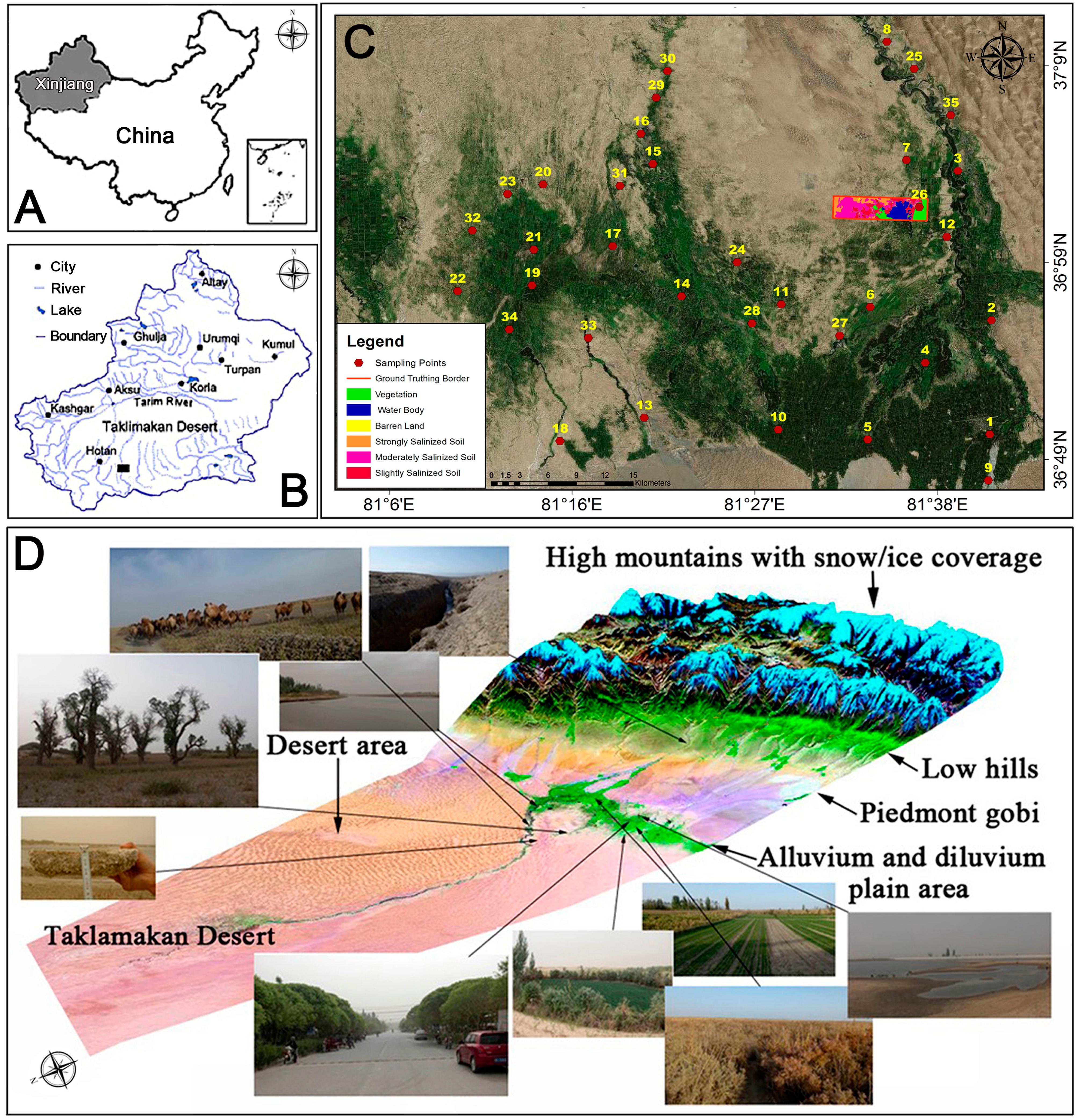
2. Study Site
3. Data
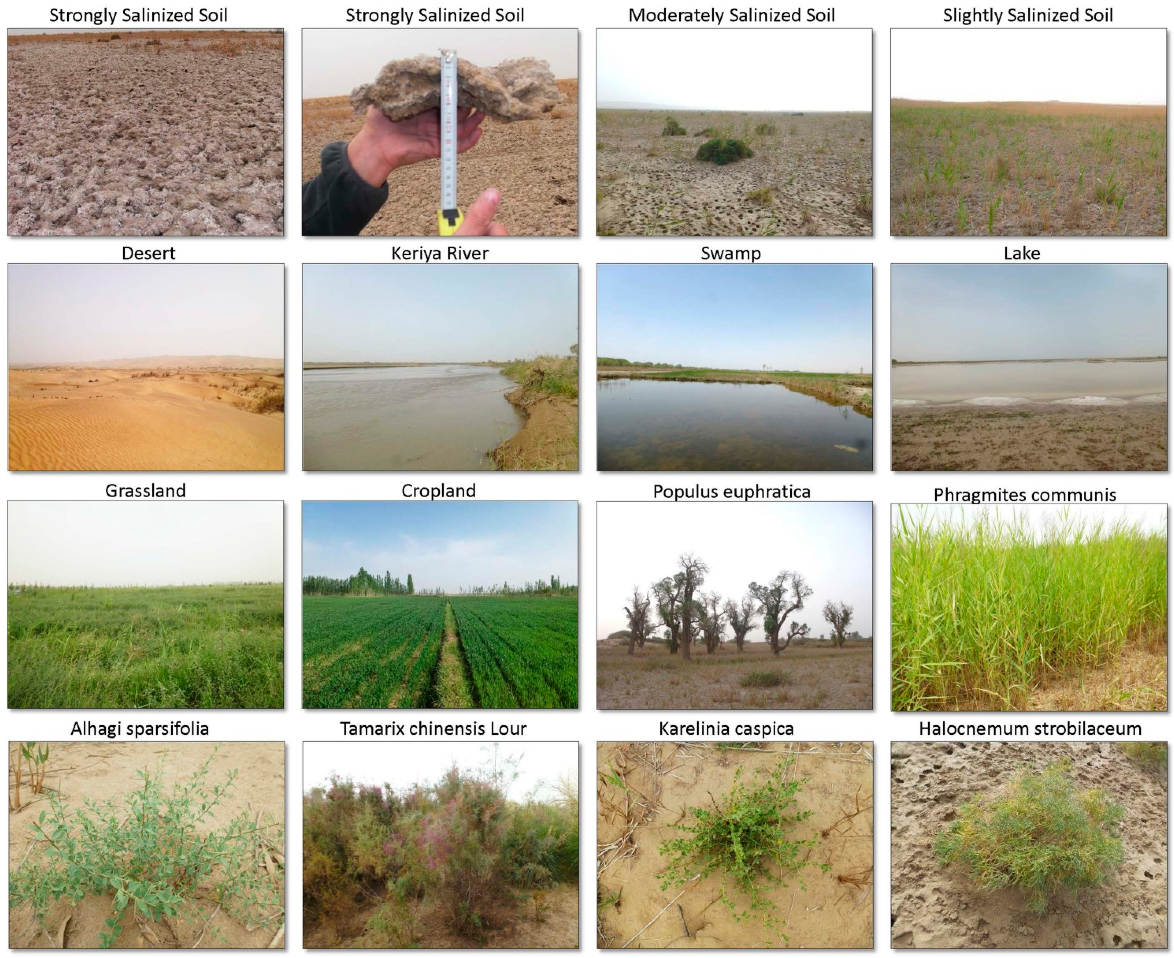
3.1. Field Data

| Abbreviation | Class | Characteristics |
|---|---|---|
| HS | Strongly Salinized soil | almost barren land with vegetation coverage less than 5%, with salt crust of 2~7 cm, top soil soluble salt ≥20 g∙kg−1, water table depth is 0.5~1.5 m |
| MS | Moderately Salinized soil | main vegetation types are Tamarix chinensis Lour, Halocnemum strobilaceum, Halostachys caspica, Phragmites communis, Alhagi pseudalhagi with vegetation coverage of around 5%~15%, with salt crust of 1~4 cm, top soil soluble salt is about 10~20 g∙kg−1, water table depth is 1~2 m |
| SS | Slightly Salinized soil | main vegetation types are Tamarix chinensis Lour, Phragmites communis, Haloxylon ammodendron, Karelinia caspica, Alhagi pseudalhagi with vegetation coverage of around 30%, with thin salt crust (around 0~2 cm), top soil soluble salt is about 5~10 g∙kg−1, water table depth is 1.4~3 m |
| WB | Water Body | river, lake, reservoir, pond and swamp |
| VG | Vegetation | grassland, cropland, Euphrates Poplar forests, dense shrubland |
| BL | Barren land | gobi, desert |
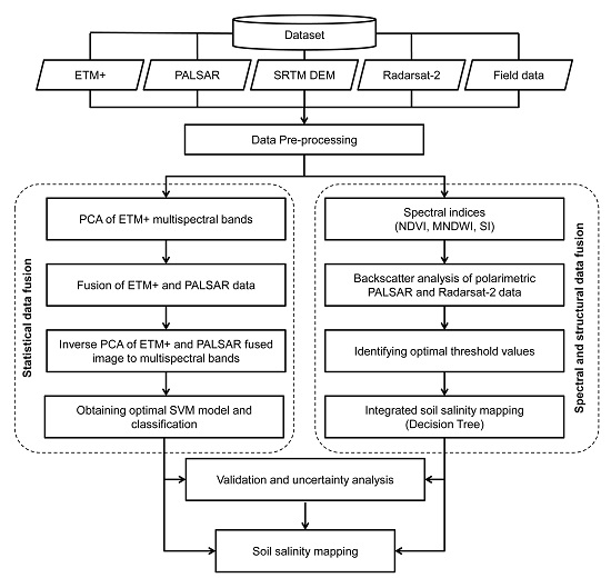
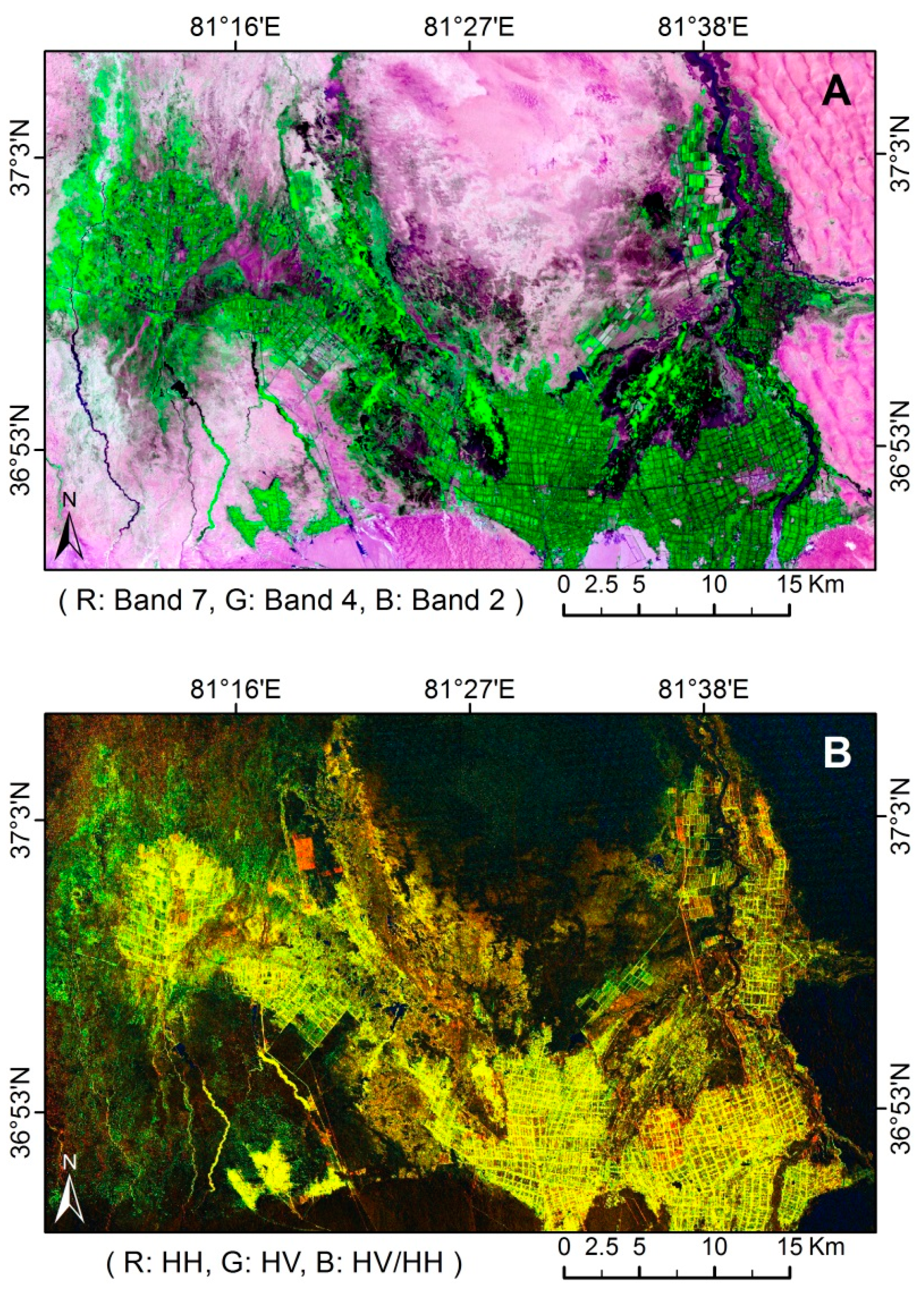
3.2. Remote Sensing Data


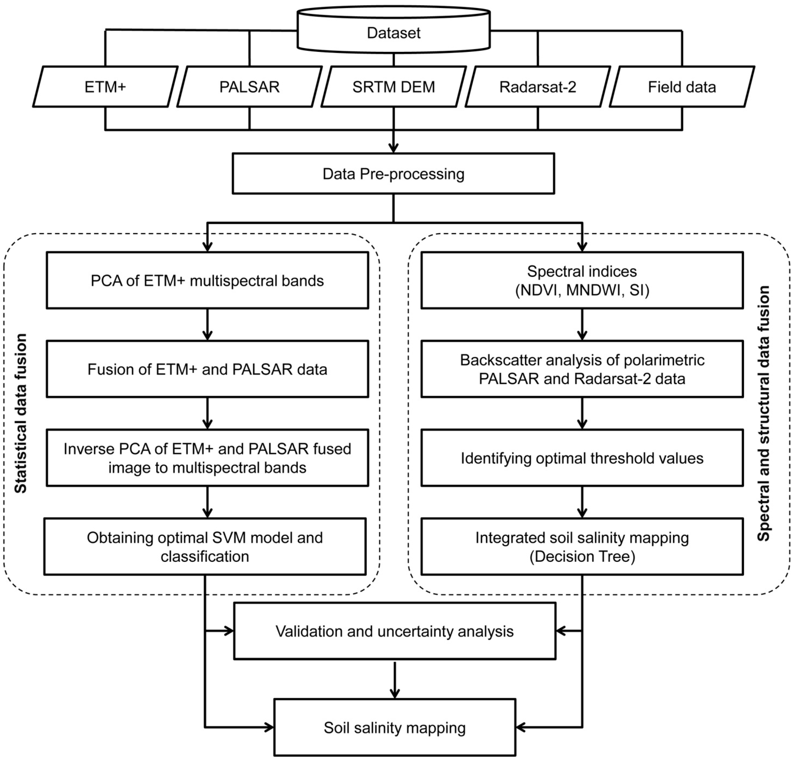
4. Methods
4.1. Spectral Indices
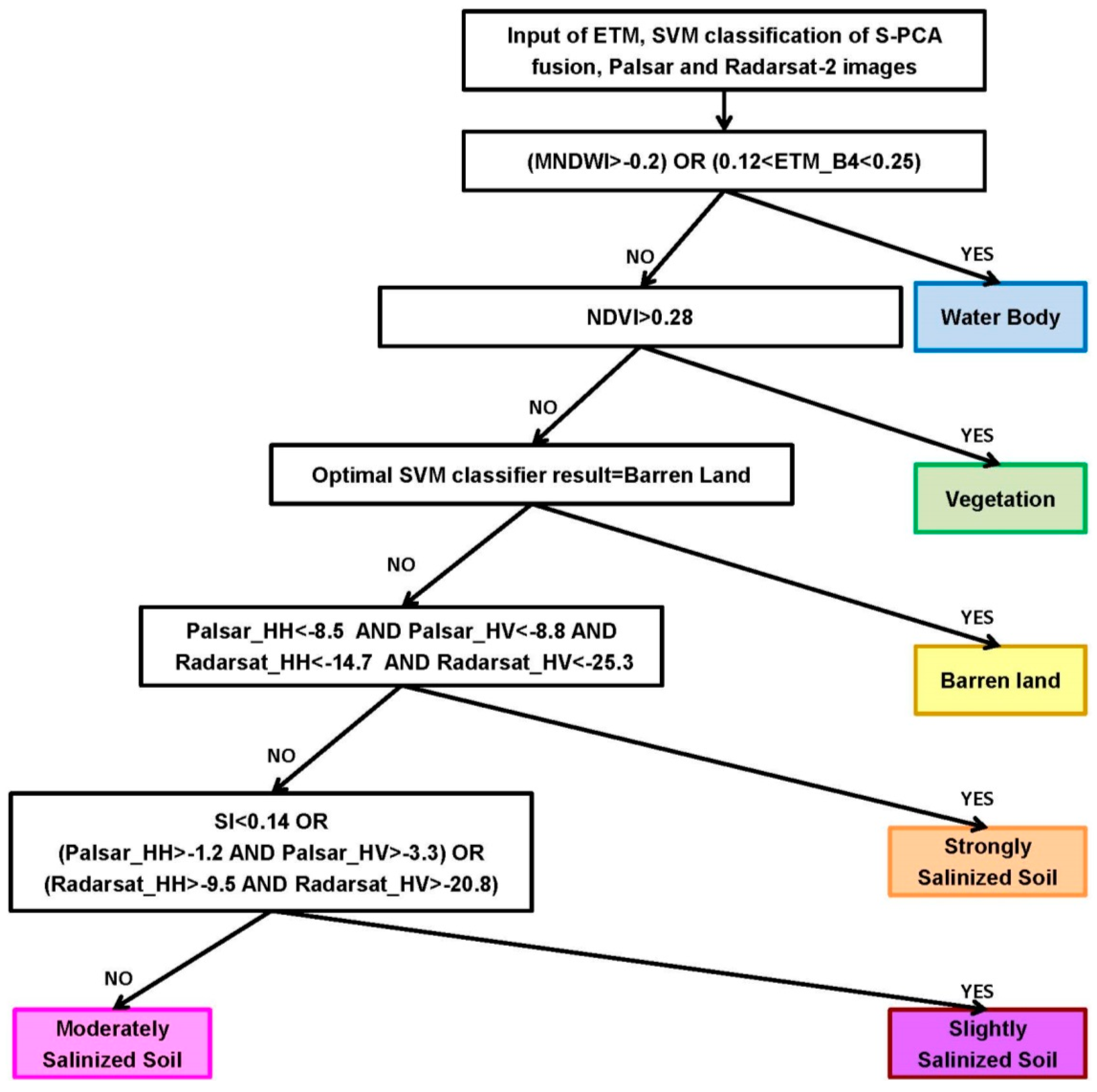
- Normalized difference vegetation index (NDVI). In the Keriya River basin, NDVI value of most vegetation types (grassland, cropland, forests and shrubland) is greater than 0.28, while the other non-vegetated land cover types were less than 0.3. Therefore, the vegetated and non-vegetated land cover types could be distinguished using NDVI threshold.
- Modified normalized difference water index (MNDWI) [35]. The MNDWI was modified after the NDWI as follows:where “Green” stands for a green band and “MIR” stands for a middle infrared band in the Landsat ETM+ images, representing ETM+ band 2 and band 5, respectively. The analysis on the study area showed that the MNDWI index could accurately separate water bodies from other land-cover types.MNDWI = (Green − MIR)/(Green + MIR)
4.2. Coregistration of Passive Reflective and Active Microwave Data
4.3. Data Fusion
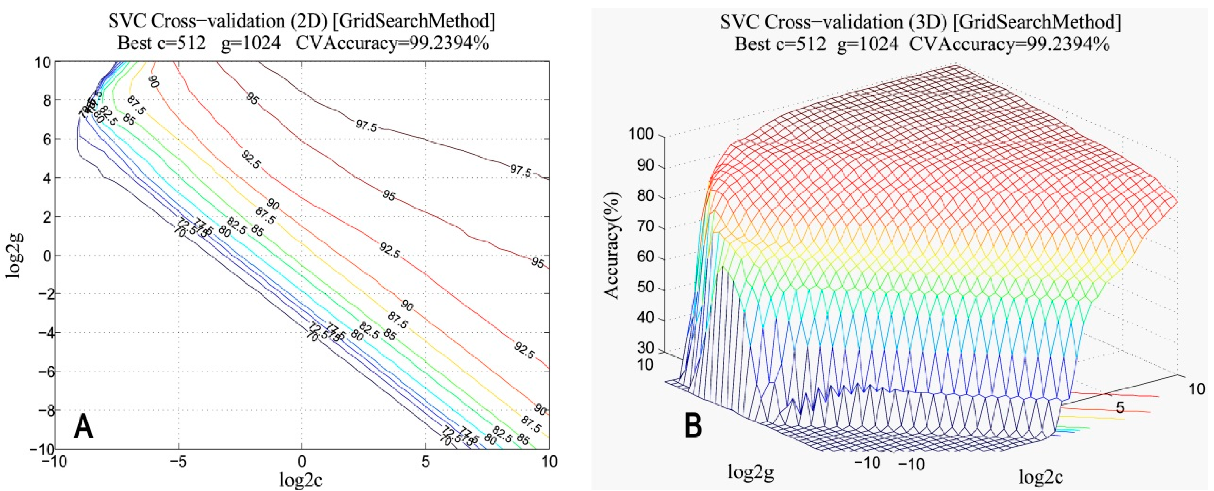
4.4. Support Vector Machine (SVM) Classification
4.5. Decision Tree
4.6. Accuracy Assessment
5. Results
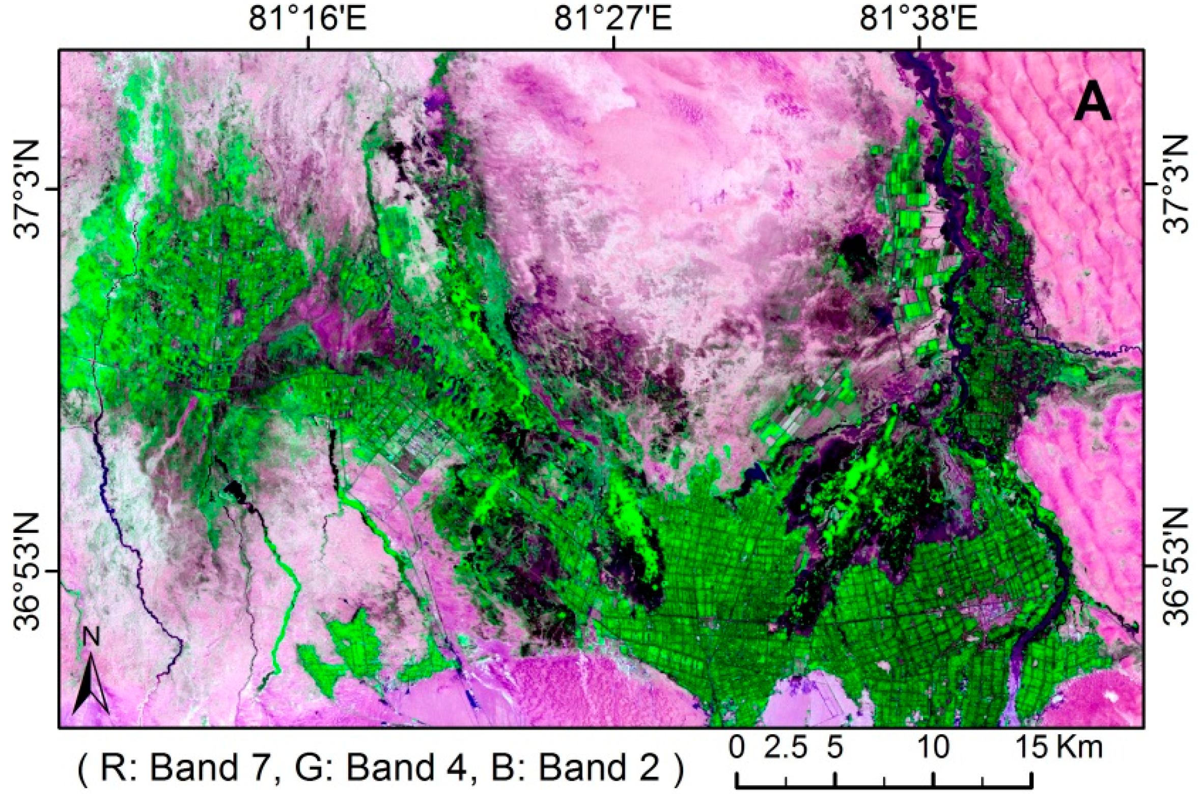
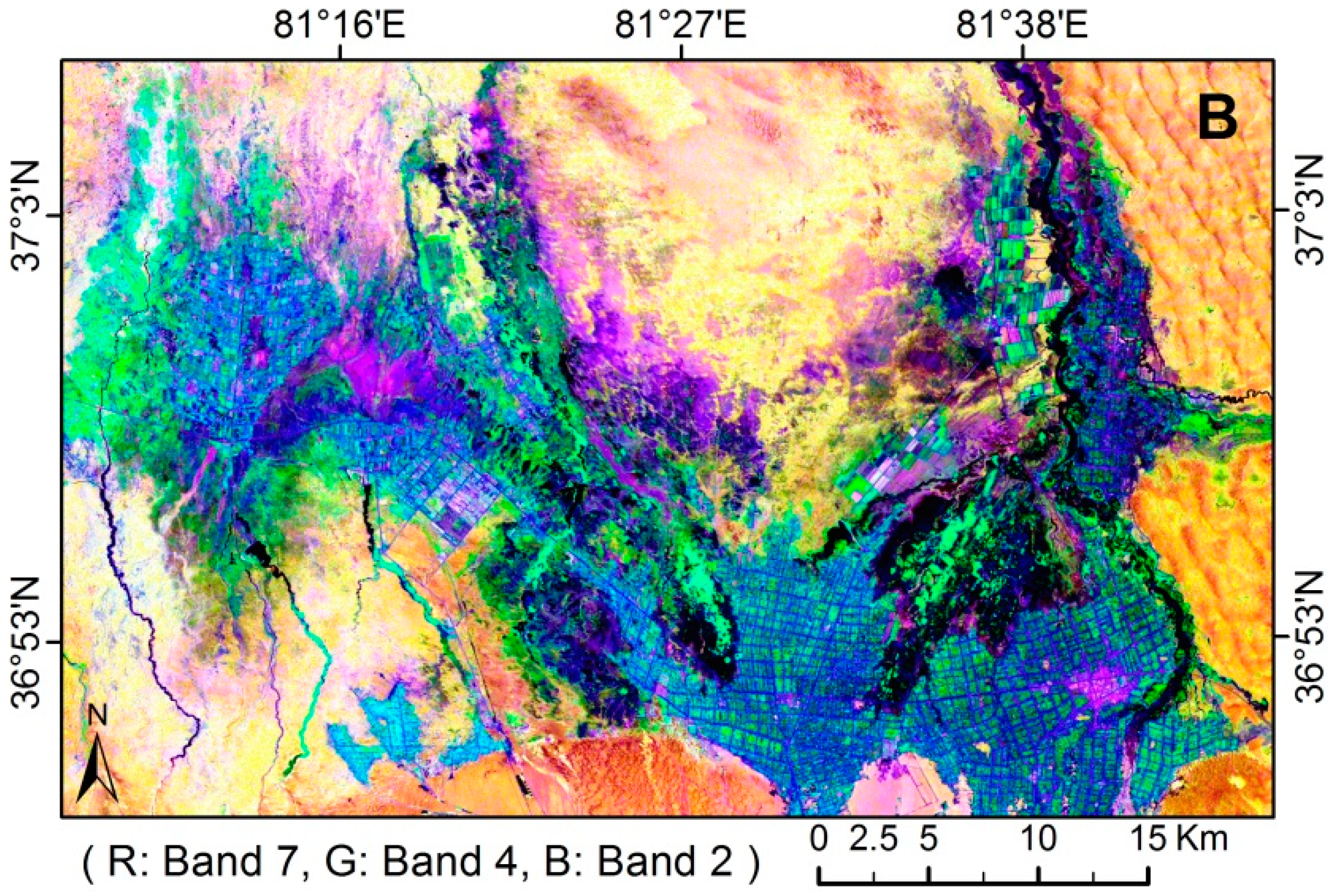
5.1. Data Fusion


5.2. SVM Classification and Accuracy
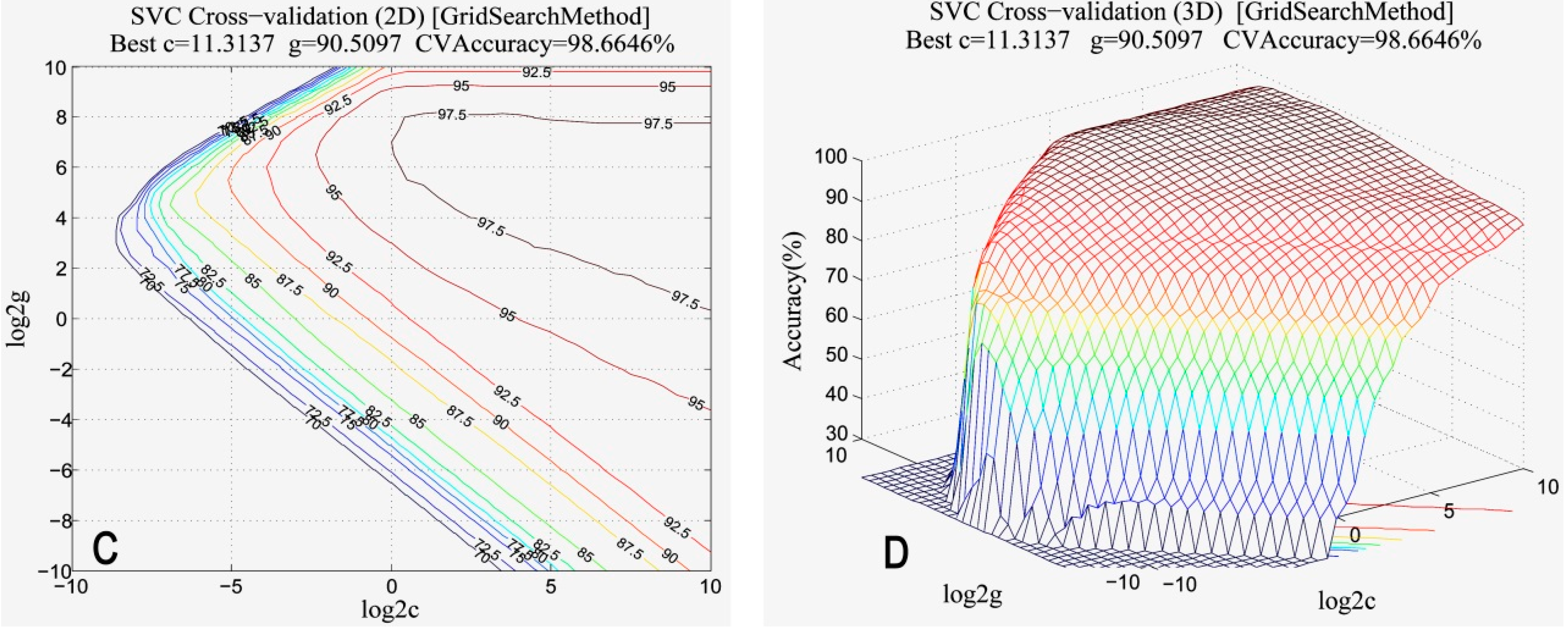
5.2.1. Optimal SVM Parameters

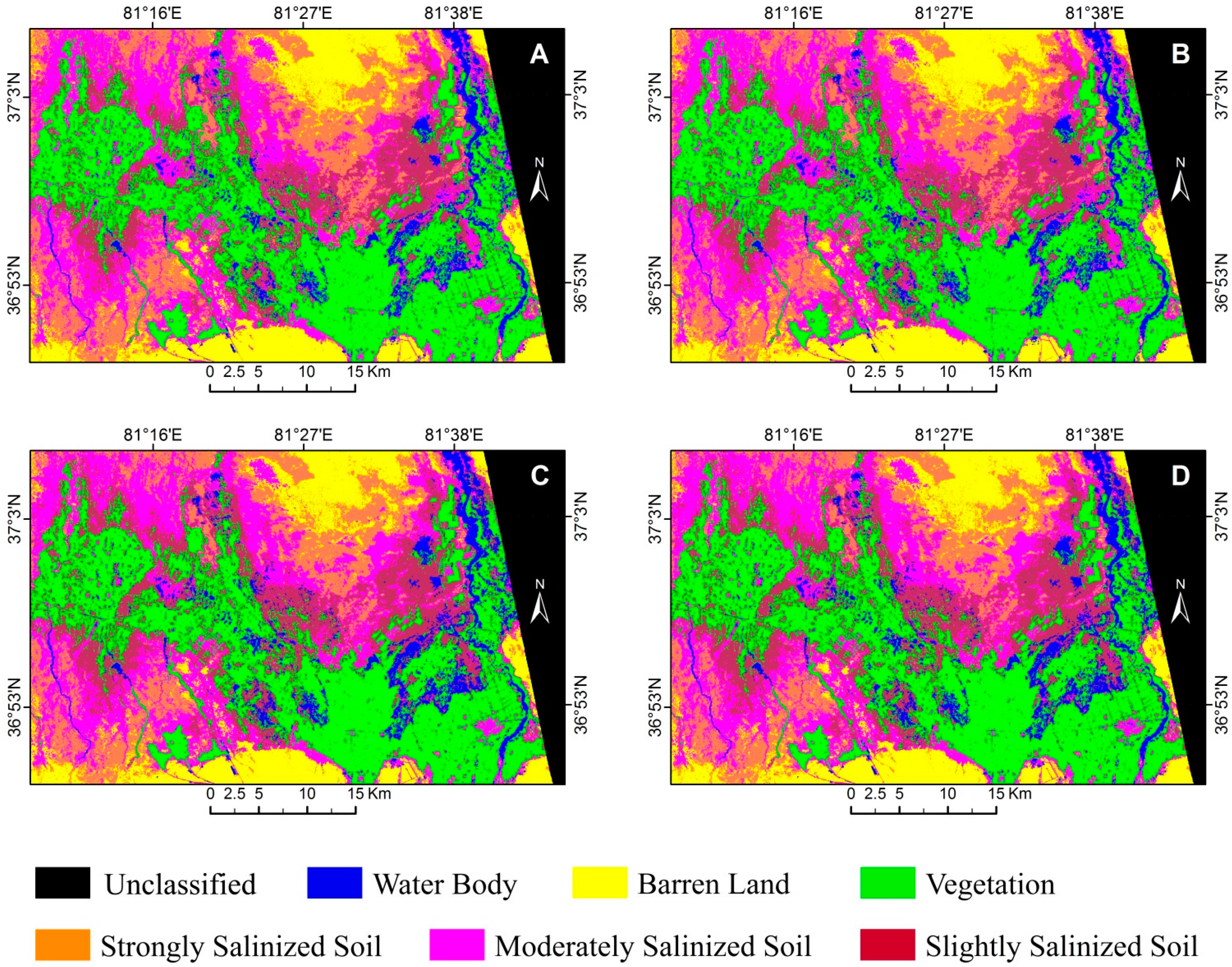
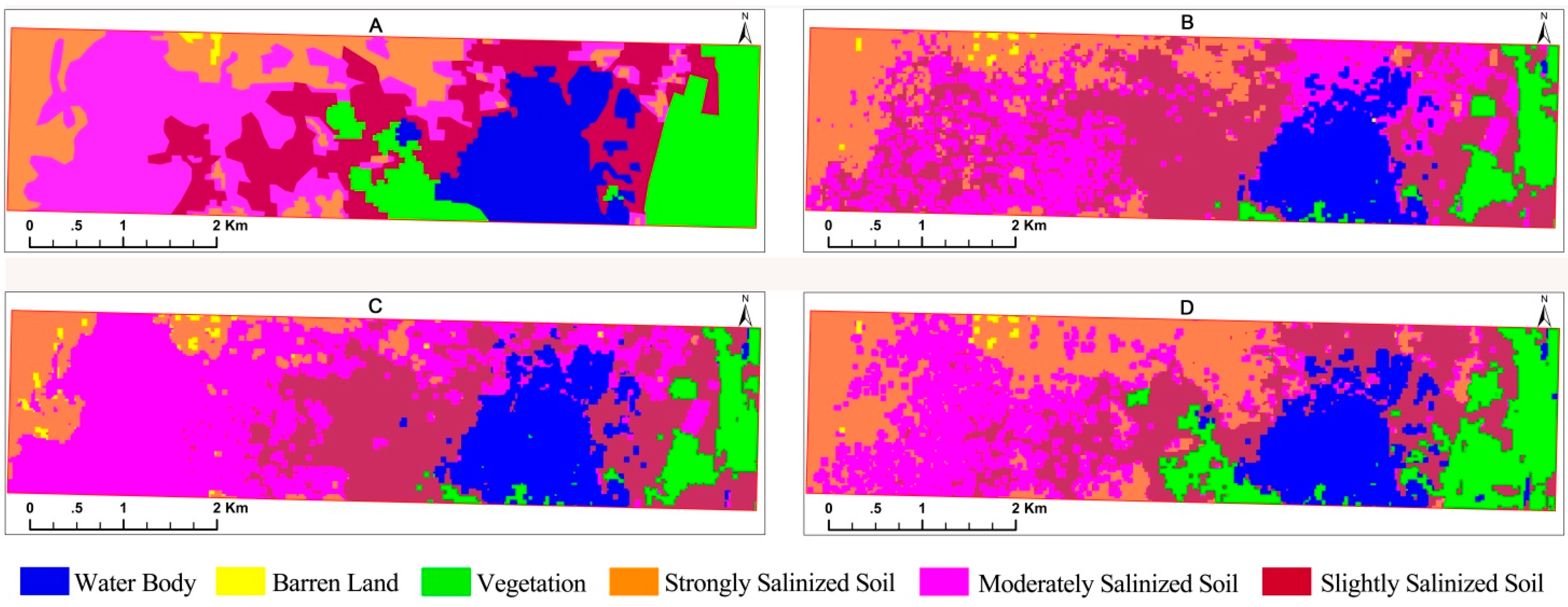
5.2.2. SVM Classification
5.2.3. Classification Accuracy
| Class | WB | BL | VG | HS | MS | SS | Prod Acc | User Acc |
|---|---|---|---|---|---|---|---|---|
| WB | 96.84 | 0 | 0 | 0 | 0.94 | 2.9 | 96.84 | 94.03 |
| BL | 0 | 96.65 | 0 | 1.4 | 0.29 | 0 | 96.65 | 97.52 |
| VG | 0.26 | 0 | 97.33 | 0 | 0 | 0 | 97.33 | 99.85 |
| HS | 0 | 1.7 | 0 | 96.31 | 19.91 | 0.06 | 96.31 | 83.58 |
| MS | 1.27 | 1.65 | 0.03 | 2.16 | 65.74 | 17.71 | 65.74 | 78.67 |
| SS | 1.64 | 0 | 2.63 | 0.13 | 13.12 | 79.33 | 79.33 | 78.57 |
| Overall Accuracy = 87.981% | ||||||||
| Kappa Coefficient = 0.8541 | ||||||||
| Class | WB | BL | VG | HS | MS | SS | Prod Acc | User Acc |
|---|---|---|---|---|---|---|---|---|
| WB | 99.08 | 0 | 0 | 0 | 1.82 | 4 | 99.08 | 91.24 |
| BL | 0 | 97.64 | 0 | 5.75 | 1.43 | 0 | 97.64 | 90.39 |
| VG | 0.2 | 0 | 98.37 | 0 | 0 | 0.52 | 98.37 | 99.43 |
| HS | 0 | 1.51 | 0.02 | 91.33 | 11.75 | 0 | 91.33 | 88.82 |
| MS | 0.03 | 0.85 | 0.08 | 2.92 | 83.28 | 13.9 | 83.28 | 85.1 |
| SS | 0.69 | 0 | 1.53 | 0 | 1.72 | 81.57 | 81.57 | 94.75 |
| Overall Accuracy = 91.25% | ||||||||
| Kappa Coefficient = 0.8938 | ||||||||
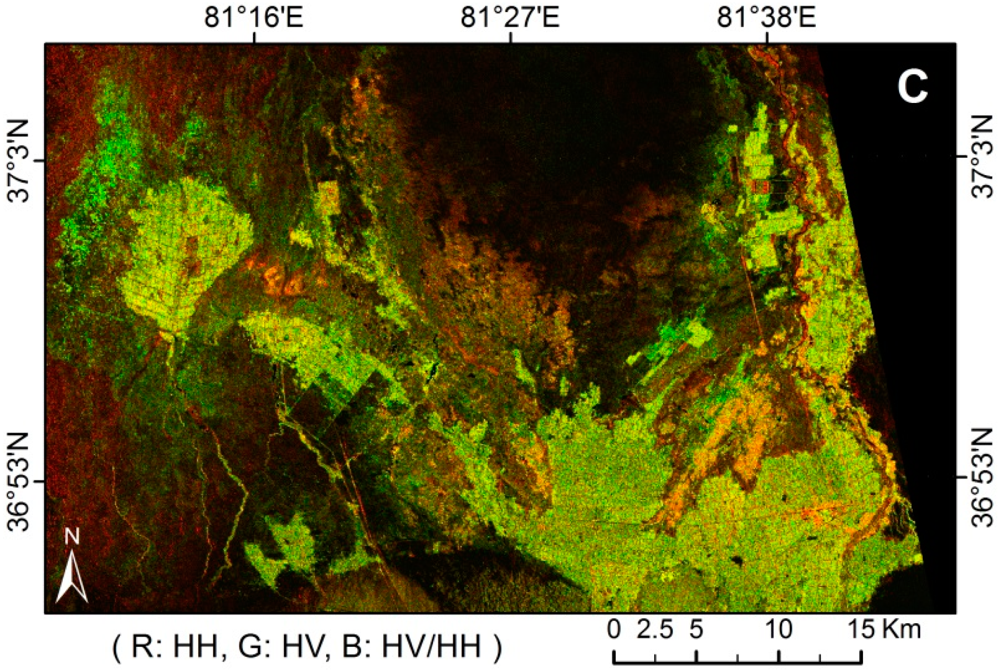
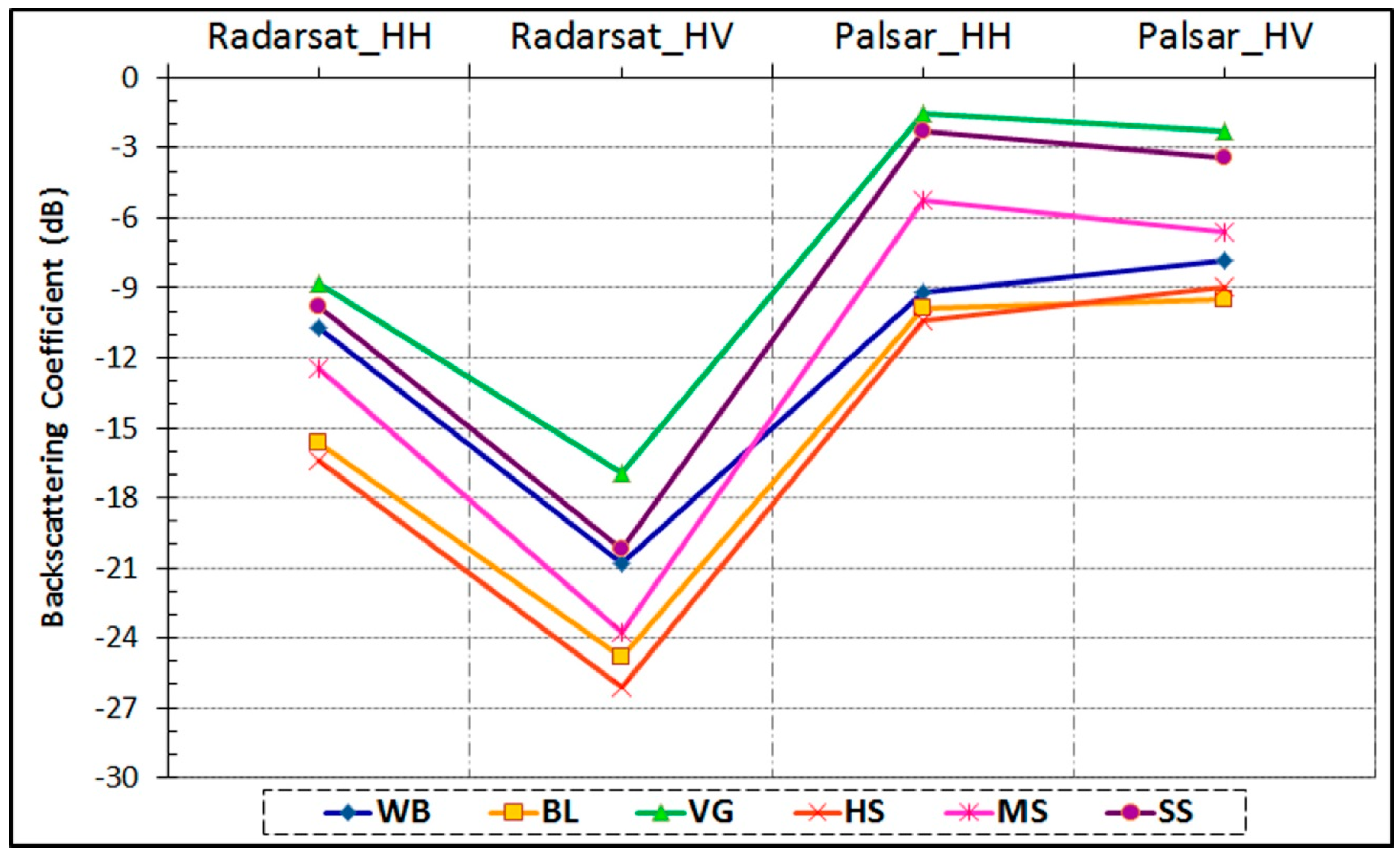
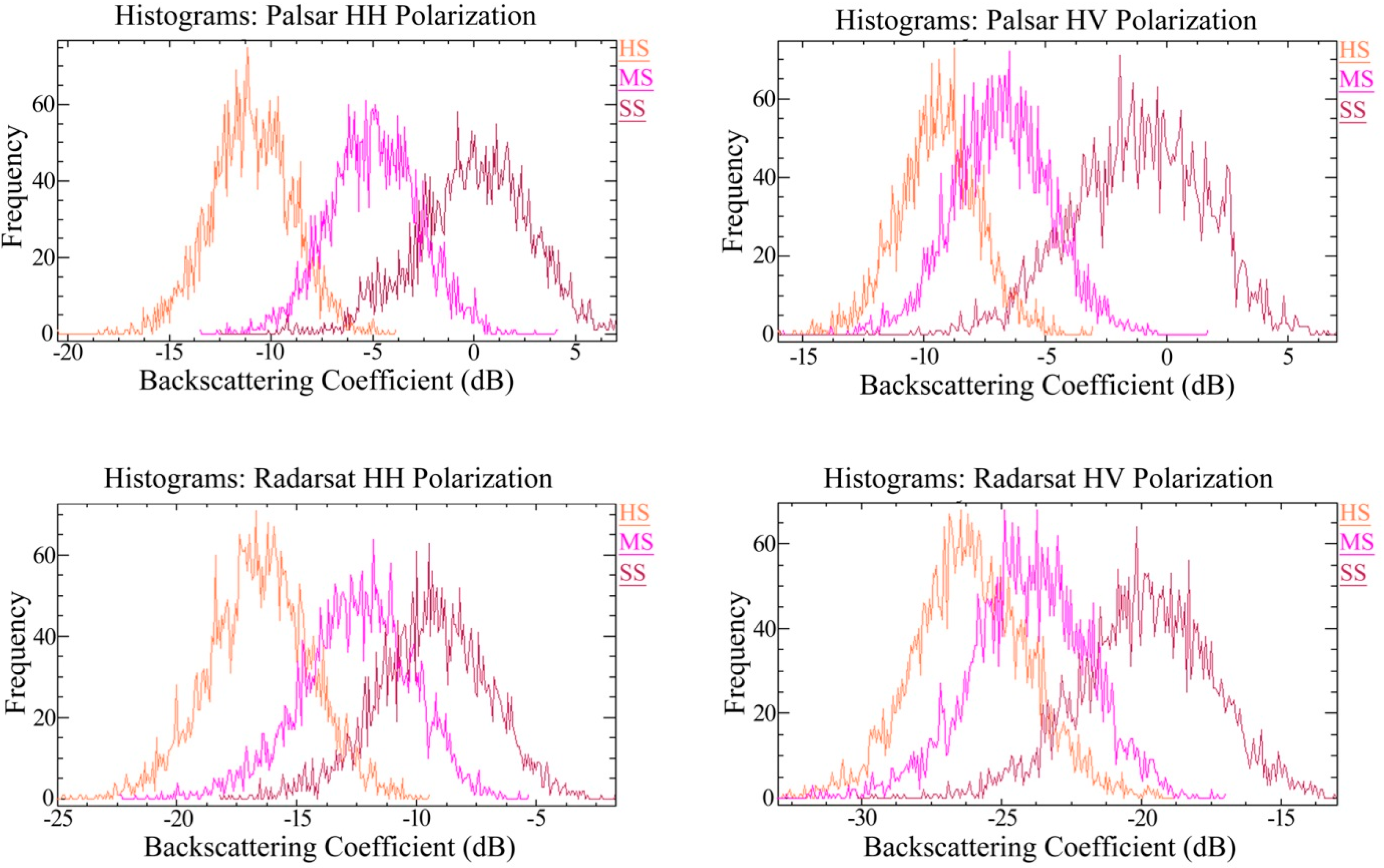
5.3. Backscattering Feature of Polarimetric PALSAR and Radarsat-2 Data


5.4. Decision Tree Classification and Accuracy


| Class | WB | BL | VG | HS | MS | SS | Prod Acc | User Acc. |
|---|---|---|---|---|---|---|---|---|
| WB | 99.57 | 0 | 0 | 0 | 1.72 | 0.64 | 99.57 | 95.85 |
| BL | 0 | 97 | 0 | 1.37 | 0.29 | 0 | 97.00 | 97.56 |
| VG | 0.23 | 0 | 97.98 | 0 | 0 | 5.45 | 97.98 | 95.36 |
| HS | 0 | 2.27 | 0.15 | 94.96 | 9.41 | 0.23 | 94.96 | 90.31 |
| MS | 0 | 0.74 | 0.05 | 3.64 | 86.85 | 9.69 | 86.85 | 87.81 |
| SS | 0.2 | 0 | 1.83 | 0.03 | 1.72 | 83.99 | 83.99 | 94.83 |
| Overall Accuracy = 93.01% | ||||||||
| Kappa Coefficient = 0.9151 | ||||||||

6. Discussion
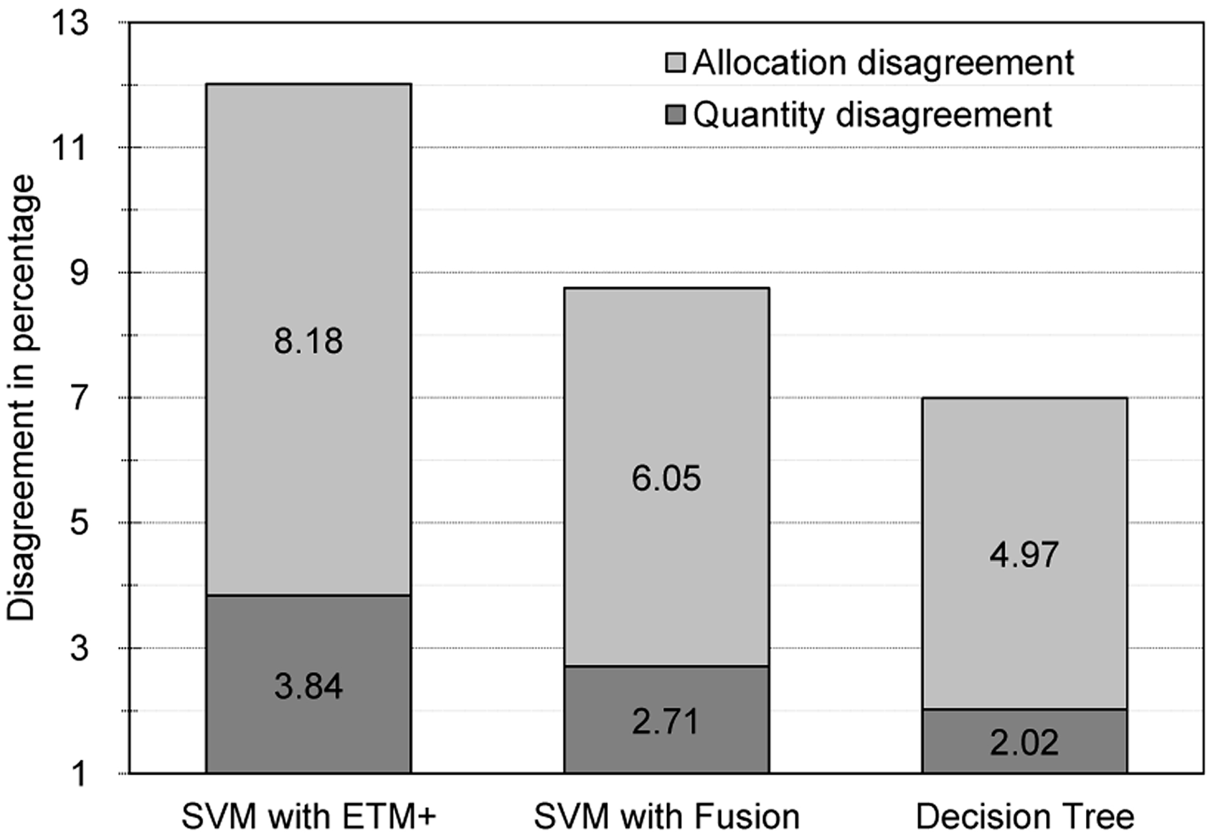
6.1. Comparison between SVM and DT Classification Method
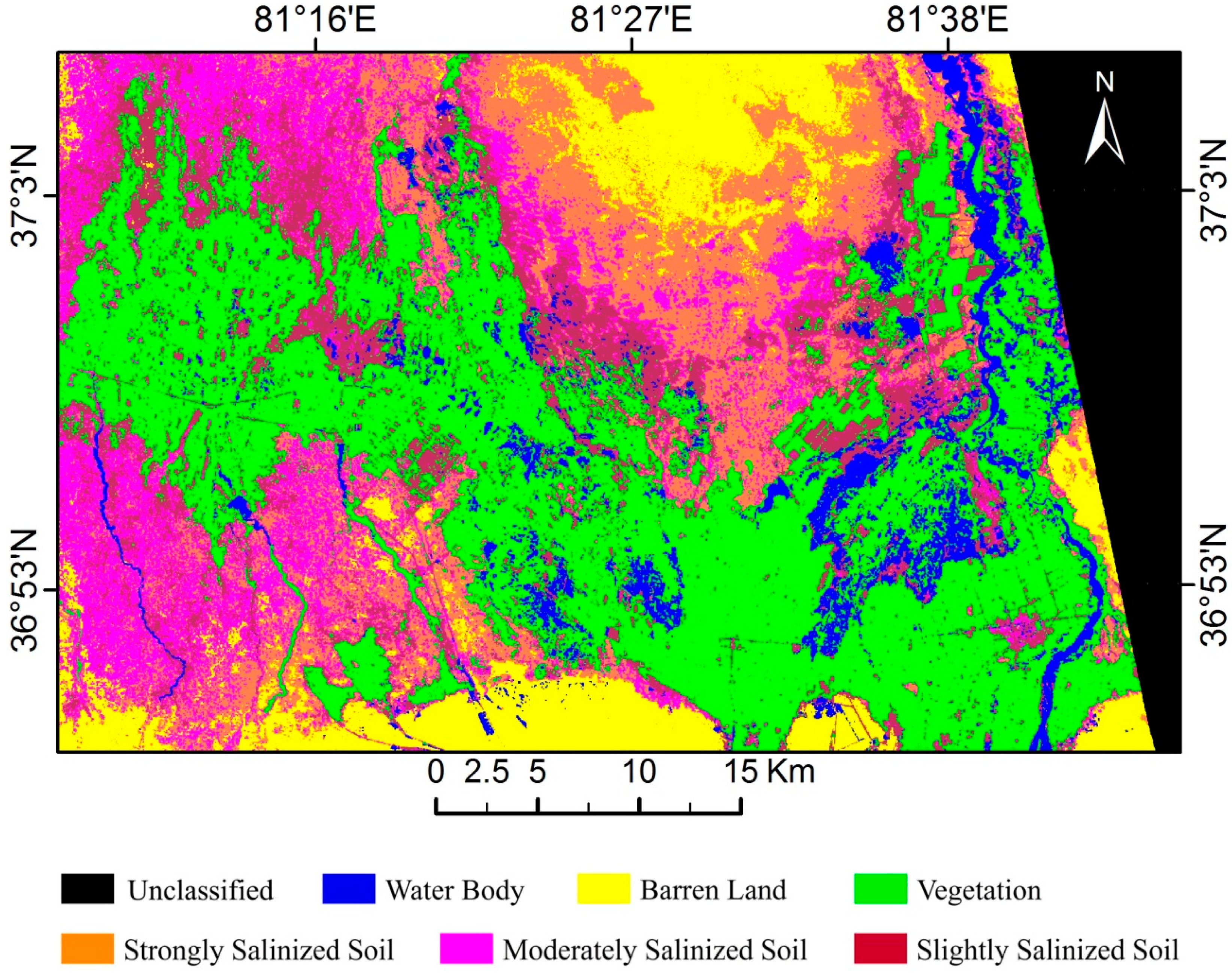
6.2. Area of Salinized Soil
| Water Body | Vegetation | Barren Land | Strongly Salinized Soil | Moderately Salinized Soil | Slightly Salinized Soil | |
|---|---|---|---|---|---|---|
| Class area (%) | 6.932 | 33.817 | 17.826 | 10.706 | 19.864 | 10.856 |
| Class area (hectare) | 13,347.48 | 65,114.68 | 34,322.92 | 20,613.84 | 38,247.56 | 20,902.40 |
6.3. Uncertainty Analysis
7. Conclusions
Acknowledgments
Author Contributions
Conflicts of Interest
References
- Farifteh, J.; Farshad, A.; George, R.J. Assessing salt-affected soils using remote sensing, solute modelling, and geophysics. Geoderma 2006, 130, 191–206. [Google Scholar] [CrossRef]
- Metternicht, G.I.; Zinck, J.A. Remote sensing of soil salinity: Potentials and constraints. Remote Sens. Environ. 2003, 85, 1–20. [Google Scholar] [CrossRef]
- Wu, J.; Li, P.; Qian, H.; Fang, Y. Assessment of soil salinization based on a low-cost method and its influencing factors in a semi-arid agricultural area, northwest China. Environ. Earth Sci. 2014, 71, 3465–3475. [Google Scholar] [CrossRef]
- Li, Y.; Zhao, K.; Ding, Y.; Ren, J. An empirical method for soil salinity and moisture inversion in West of Jilin. In Proceedings of the 2013 the International Conference on Remote Sensing, Environment and Transportation Engineering (RSETE 2013), Nanjing, China, 26–28 July 2013; pp. 19–21.
- Wang, H.; Jia, G. Satellite-based monitoring of decadal soil salinization and climate effects in a semi-arid region of China. Adv. Atmos. Sci. 2012, 29, 1089–1099. [Google Scholar] [CrossRef]
- Metternicht, G.I. Analysing the relationship between ground-based reflectance and environmental indicators of salinity processes in the Cochabamba valleys (Bolivia). Int. J. Ecol. Environ. Sci. 1998, 24, 359–370. [Google Scholar]
- Metternicht, G.; Zinck, J.A. Spatial discrimination of salt- and sodium-affected soil surfaces. Int. J. Remote Sens. 1997, 18, 2571–2586. [Google Scholar] [CrossRef]
- Nawar, S.; Buddenbaum, H.; Hill, J. Digital mapping of soil properties using multivariate statistical analysis and ASTER data in an arid region. Remote Sens. 2015, 7, 1181–1205. [Google Scholar] [CrossRef]
- Allbed, A.; Kumar, L.; Sinha, P. Mapping and modelling spatial variation in soil salinity in the Al Hassa Oasis based on remote sensing indicators and regression techniques. Remote Sens. 2014, 6, 1137–1157. [Google Scholar] [CrossRef]
- Eldeiry, A.A.; Garcia, L.A. Comparison of ordinary kriging, regression kriging, and cokriging techniques to estimate soil salinity using Landsat images. J. Irrig. Drain. Eng. 2010, 136, 355–364. [Google Scholar] [CrossRef]
- Aldabaa, A.A.A.; Weindorf, D.C.; Chakraborty, S.; Sharma, A.; Li, B. Combination of proximal and remote sensing methods for rapid soil salinity quantification. Geoderma 2015, 239, 34–46. [Google Scholar] [CrossRef]
- Masoud, A.A. Predicting salt abundance in slightly saline soils from Landsat ETM+ imagery using spectral mixture analysis and soil spectrometry. Geoderma 2014, 217, 45–56. [Google Scholar] [CrossRef]
- Nawar, S.; Buddenbaum, H.; Hill, J.; Kozak, J. Modeling and mapping of soil salinity with reflectance spectroscopy and Landsat data using two quantitative methods (PLSR and MARS). Remote Sens. 2014, 6, 10813–10834. [Google Scholar] [CrossRef]
- Sidike, A.; Zhao, S.; Wen, Y. Estimating soil salinity in Pingluo County of China using QuickBird data and soil reflectance spectra. Int. J. Appl. Earth Obs. Geoinf. 2014, 26, 156–175. [Google Scholar] [CrossRef]
- Fan, X.; Liu, Y.; Tao, J.; Weng, Y. Soil salinity retrieval from advanced multi-spectral sensor with partial least square regression. Remote Sens. 2015, 7, 488–511. [Google Scholar] [CrossRef]
- Jin, P.; Li, P.; Wang, Q.; Pu, Z. Developing and applying novel spectral feature parameters for classifying soil salt types in arid land. Ecol. Indic. 2015, 54, 116–123. [Google Scholar] [CrossRef]
- Sreenivas, K.; Venkataratnam, L.; Rao, P.V.N. Dielectric properties of salt-affected soils. Int. J. Remote Sens. 1995, 16, 641–649. [Google Scholar] [CrossRef]
- Gharechelou, S.; Tateishi, R.; Sumantyo, J. Interrelationship analysis of L-band backscattering intensity and soil dielectric constant for soil moisture retrieval using PALSAR data. Adv. Remote Sens. 2015, 4, 15–24. [Google Scholar] [CrossRef]
- Rhoades, J.D. Electrical Conductivity Methods for Measuring and Mapping Soil Salinity; Academic Press: Waltham, MA, USA, 1993. [Google Scholar]
- Shao, Y.; Hu, Q.; Guo, H.; Lu, Y.; Dong, Q.; Han, C. Effect of dielectric properties of moist salinized soils on backscattering coefficients extracted from RADARSAT image. IEEE Trans. Geosci. Remote Sens. 2003, 41, 1879–1888. [Google Scholar] [CrossRef]
- Ghulam, A.; Porton, I.; Freeman, K. Detecting subcanopy invasive plant species in tropical rainforest by integrating optical and microwave (InSAR/PolInSAR) remote sensing data, and a decision tree algorithm. ISPRS J. Photogramm. Remote Sens. 2014, 88, 174–192. [Google Scholar] [CrossRef]
- Ghulam, A. Monitoring tropical forest degradation in Betampona Nature Reserve, Madagascar, using multisource remote sensing data fusion. IEEE J. Sel. Top. Appl. Earth Obs. Remote Sens. 2014, 7, 1–12. [Google Scholar] [CrossRef]
- Mu, Q.; Zi-an, Z.; Hong, M. Survey on the Arable Land Resource of Xinjiang Based on Remote Sensing; Science and Technology Publishing House of Xinjiang: Urumqi, China, 2005. [Google Scholar]
- Tashpolat, T.; Fei, Z.; Jianli, D. Study on the spatial information on salinized soil of typical oases in arid areas. Arid L. Geogr. 2007, 4, 544–551. [Google Scholar]
- Yang, X. The oases along the Keriya River in the Taklamakan Desert, China, and their evolution since the end of the last glaciation. Environ. Geol. 2001, 41, 314–320. [Google Scholar]
- Ling, H.; Xu, H.; Zhang, Q. Nonlinear analysis of runoff change and climate factors in the headstream of Keriya River, Xinjiang. Geogr. Res. 2012, 31, 792–802. (in Chinese). [Google Scholar]
- Yuquan, L. The climatic characteristics and its changing tendency in the Taklimakan desert. J. Desert Res. 1990, 2, 9–19. [Google Scholar]
- Scaramuzza, P.; Micijevic, E.; Chander, G. SLC Gap-Filled Products Phase One Methodology. Available online: https://landsat.usgs.gov/documents/SLC_Gap_Fill_Methodology.pdf (accessed on 13 April 2015).
- Lopes, A.; Touzi, R.; Nezry, E. Adaptive speckle filters and scene heterogeneity. IEEE Trans. Geosci. Remote Sens. 1990, 28, 992–1000. [Google Scholar] [CrossRef]
- Holecz, F.; Meier, E.; Piesbergen, J.; Nisch, D.; Moreira, J. Rigorous derivation of backscattering coefficient. IEEE Geosc. Remote Sens. Soc. Newsletter. 1994, 92, 6–14. [Google Scholar]
- Sarmap, S.A. Synthetic Aperture Radar and SARscape: SAR Guidebook; Sarmap SA: Purasca, Switzerland, 2009. [Google Scholar]
- Ulaby, F.T.; Dobson, M.C. Handbook of Radar Scattering Statistics for Terrain; Artech House: Norwood, MA, USA, 1989. [Google Scholar]
- Chander, G.; Markham, B.L.; Helder, D.L. Summary of current radiometric calibration coefficients for Landsat MSS, TM, ETM+, and EO-1 ALI sensors. Remote Sens. Environ. 2009, 113, 893–903. [Google Scholar] [CrossRef]
- Vermote, E.F.; Tanré, D.; Deuzé, J.L.; Herman, M.; Morcrette, J.J. Second simulation of the satellite signal in the solar spectrum, 6S: An overview. IEEE Trans. Geosci. Remote Sens. 1997, 35, 675–686. [Google Scholar] [CrossRef]
- Xu, H. A Study on information extraction of water body with the Modified Normalized Difference Water Index (MNDWI). J. Remote Sens. 2005, 9, 589–595. [Google Scholar]
- Khan, N.M.; Rastoskuev, V.V.; Sato, Y.; Shiozawa, S. Assessment of hydrosaline land degradation by using a simple approach of remote sensing indicators. Agri. Water Manag. 2005, 77, 96–109. [Google Scholar] [CrossRef]
- Khan, N.M.; Sato, Y. Monitoring hydro-salinity status and its impact in irrigated semi-arid areas using IRS-1B LISS-II data. Asian J. Geoinform 2001, 1, 63–73. [Google Scholar]
- Wang, F.; Chen, X.; Luo, G.; Ding, J.; Chen, X. Detecting soil salinity with arid fraction integrated index and salinity index in feature space using Landsat TM imagery. J. Arid Land 2013, 5, 340–353. [Google Scholar] [CrossRef]
- Douaoui, A.E.K.; Nicolas, H.; Walter, C. Detecting salinity hazards within a semiarid context by means of combining soil and remote-sensing data. Geoderma 2006, 134, 217–230. [Google Scholar] [CrossRef]
- Khan, N.M.; Sato, Y. Environmental land degradation assessment in semi-arid Indus basin area using IRS-1B LISS-II data. In Proceedings of the IEEE 2001 International Geoscience and Remote Sensing Symposium, Sydney, Ausralia, 9–13 July 2001; Volume 5, pp. 2100–2102.
- Campbell, N.A.; Wu, X. Gradient cross correlation for sub-pixel matching. In Proceedings of the Congress of the International Society for Photogrammetry and Remote Sensing, Beijing, China, 7 July 2008; pp. 1065–1070.
- Zhou, J.; Civco, D.L.; Silander, J.A. A wavelet transform method to merge Landsat TM and SPOT panchromatic data. Int. J. Remote Sens. 1998, 19, 743–757. [Google Scholar] [CrossRef]
- Vapnik, V.N. The Nature of Statistical Learning Theory; Springer-Verlag: Berlin, Germany, 1995. [Google Scholar]
- Keerthi, S.S.; Lin, C.-J. Asymptotic behaviors of support vector machines with Gaussian kernel. Neural Comput. 2003, 15, 1667–1689. [Google Scholar] [CrossRef] [PubMed]
- Chang, C.-C.; Lin, C.-J. LIBSVM: A library for support vector machines. ACM Trans. Intell. Syst. Technol. 2011, 2, 1–27. [Google Scholar] [CrossRef]
- Andrew, M.; Ustin, S.L. The role of environmental context in mapping invasive plants with hyperspectral image data. Remote Sens. Environ. 2008, 112, 4301–4317. [Google Scholar] [CrossRef]
- Friedl, M.A.; Brodley, C.E. Decision tree classification of land cover from remotely sensed data. Remote Sens. Environ. 1997, 61, 399–409. [Google Scholar] [CrossRef]
- Hansen, M.; Dubayah, R.; Defries, R. Classification trees: An alternative to traditional land cover classifiers. Int. J. Remote Sens. 1996, 17, 1075–1081. [Google Scholar] [CrossRef]
- Elnaggar, A.A.; Noller, J.S. Application of remote-sensing data and decision-tree analysis to mapping salt-affected soils over large areas. Remote Sens. 2009, 2, 151–165. [Google Scholar] [CrossRef]
- Pontius, R.G.; Millones, M. Death to Kappa: Birth of quantity disagreement and allocation disagreement for accuracy assessment. Int. J. Remote Sens. 2011, 32, 4407–4429. [Google Scholar] [CrossRef]
- Congalton, R.G.; Green, K. Assessing the Accuracy of Remotely Sensed Data: Principles and Practices; CRC press: Boca Raton, FL, USA, 2010. [Google Scholar]
- Congalton, R.G. A review of assessing the accuracy of classifications of remotely sensed data. Remote Sens. Environ. 1991, 37, 35–46. [Google Scholar] [CrossRef]
- Badreldin, N.; Goossens, R. Monitoring land use/land cover change using multi-temporal Landsat satellite images in an arid environment: A case study of El-Arish, Egypt. Arab. J. Geosci. 2014, 7, 1671–1681. [Google Scholar] [CrossRef]
- Jia, H.F.; Liu, X. Principle and Application of Environmental Remote Sensing; Tsinghua University Press: Beijing, China, 2006. [Google Scholar]
© 2015 by the authors; licensee MDPI, Basel, Switzerland. This article is an open access article distributed under the terms and conditions of the Creative Commons Attribution license (http://creativecommons.org/licenses/by/4.0/).
Share and Cite
Nurmemet, I.; Ghulam, A.; Tiyip, T.; Elkadiri, R.; Ding, J.-L.; Maimaitiyiming, M.; Abliz, A.; Sawut, M.; Zhang, F.; Abliz, A.; et al. Monitoring Soil Salinization in Keriya River Basin, Northwestern China Using Passive Reflective and Active Microwave Remote Sensing Data. Remote Sens. 2015, 7, 8803-8829. https://doi.org/10.3390/rs70708803
Nurmemet I, Ghulam A, Tiyip T, Elkadiri R, Ding J-L, Maimaitiyiming M, Abliz A, Sawut M, Zhang F, Abliz A, et al. Monitoring Soil Salinization in Keriya River Basin, Northwestern China Using Passive Reflective and Active Microwave Remote Sensing Data. Remote Sensing. 2015; 7(7):8803-8829. https://doi.org/10.3390/rs70708803
Chicago/Turabian StyleNurmemet, Ilyas, Abduwasit Ghulam, Tashpolat Tiyip, Racha Elkadiri, Jian-Li Ding, Matthew Maimaitiyiming, Abdulla Abliz, Mamat Sawut, Fei Zhang, Abdugheni Abliz, and et al. 2015. "Monitoring Soil Salinization in Keriya River Basin, Northwestern China Using Passive Reflective and Active Microwave Remote Sensing Data" Remote Sensing 7, no. 7: 8803-8829. https://doi.org/10.3390/rs70708803