
River Detection in Remotely Sensed Imagery Using Gabor Filtering and Path Opening

 , ,
, ,
Abstract
:
1. Introduction
2. Method
2.1. Pre-Process
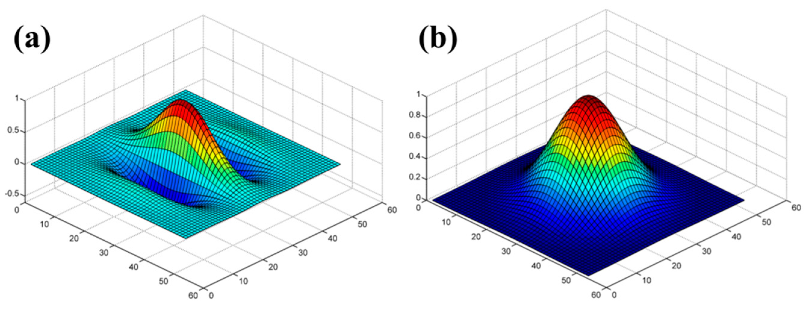
2.2. Gabor Filtering

2.3. Path Opening


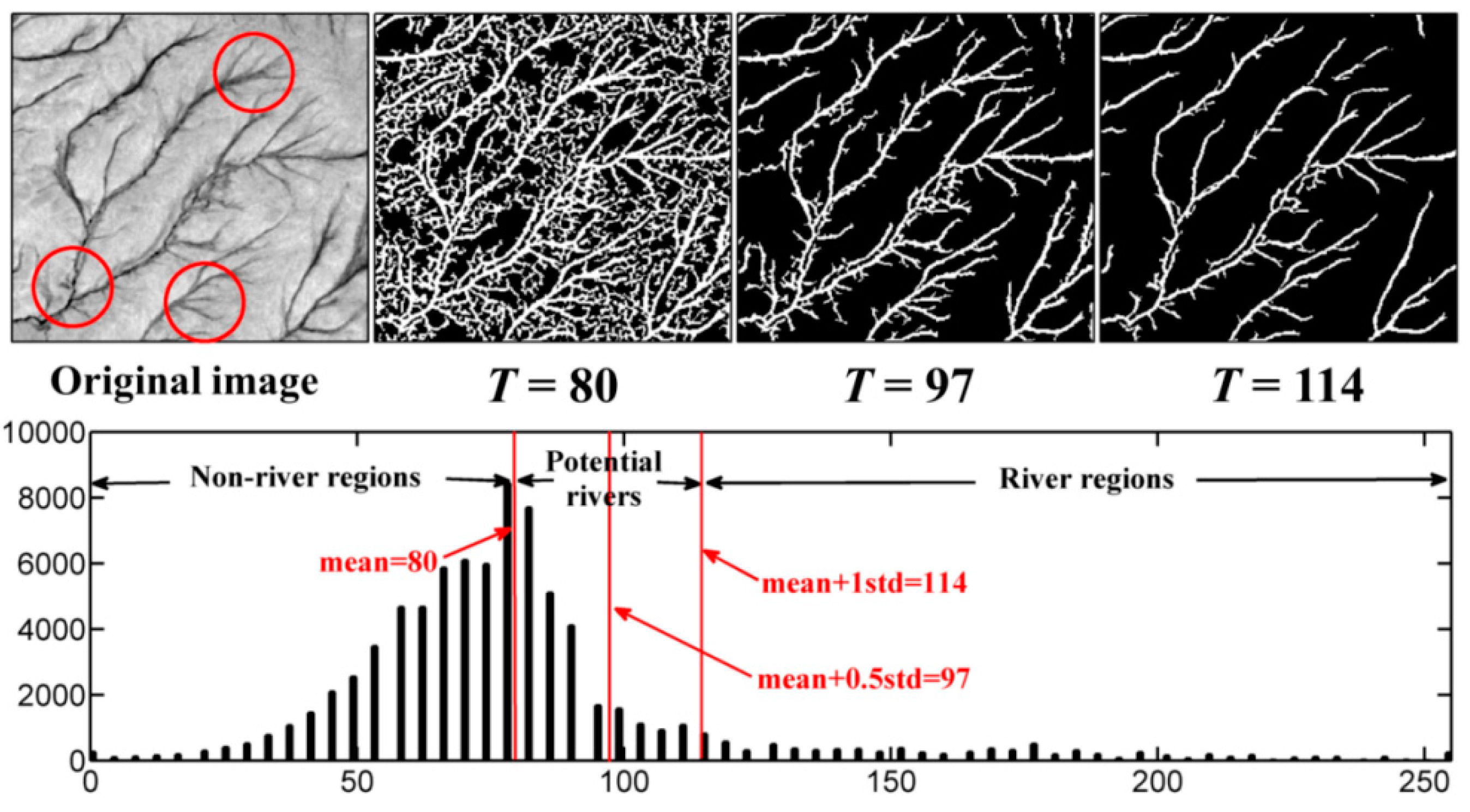
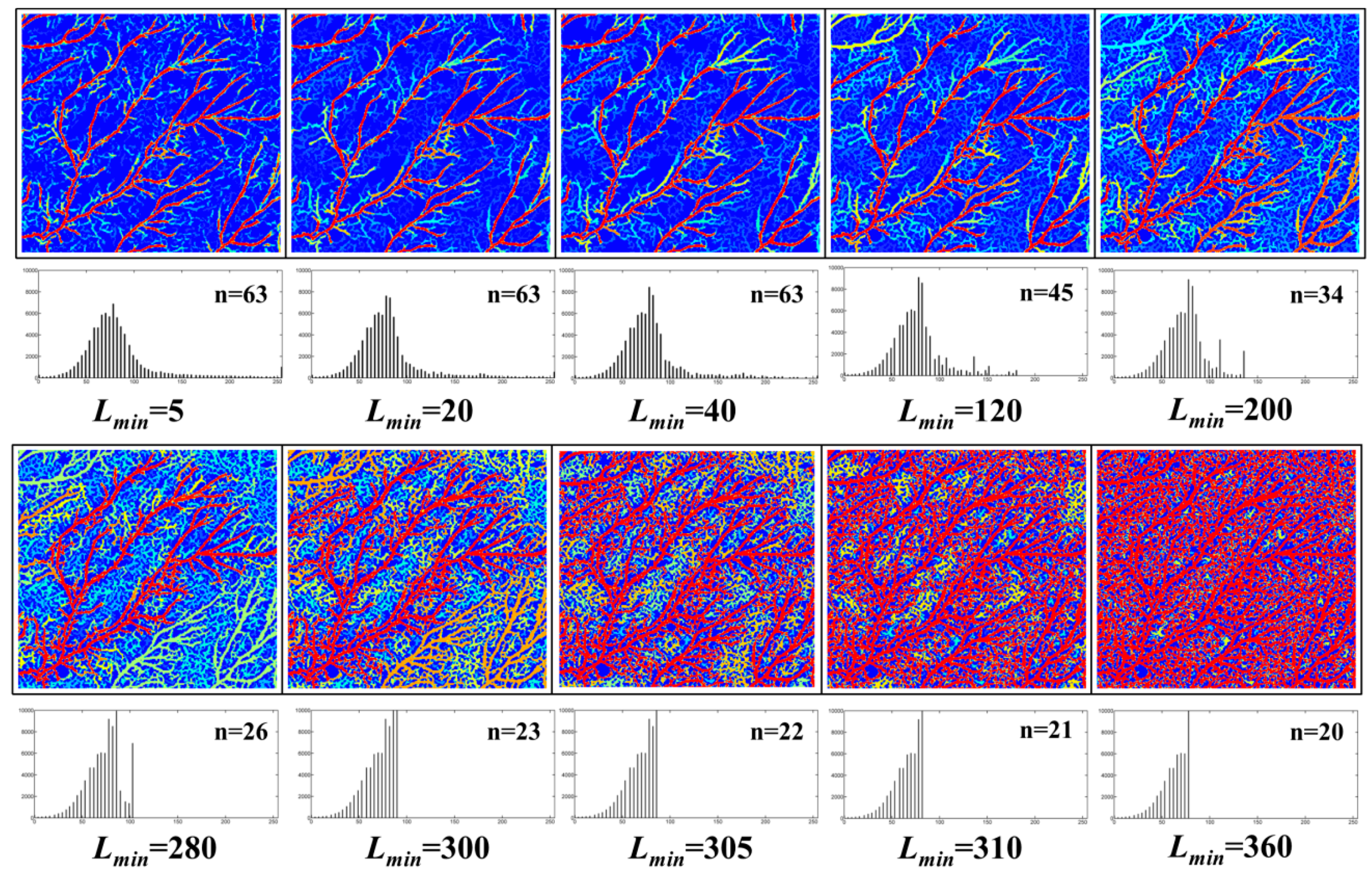
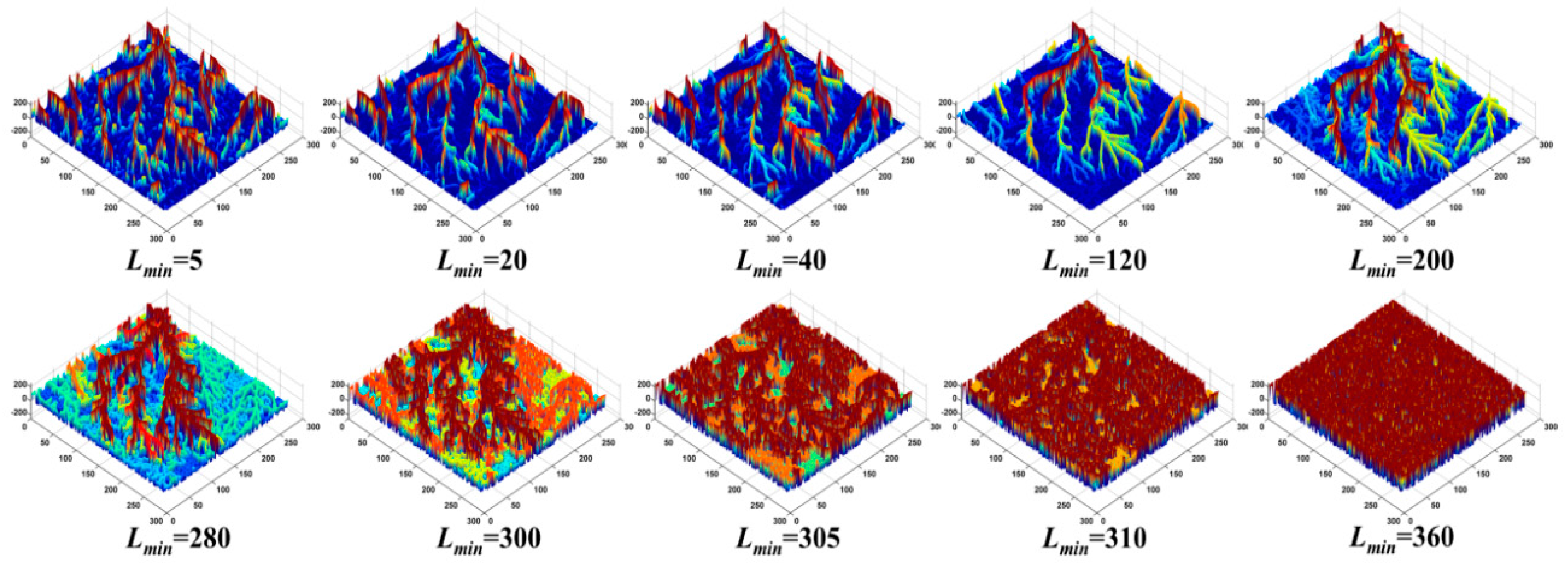
2.4. Thresholding

3. Experimental Results
3.1. Implementation
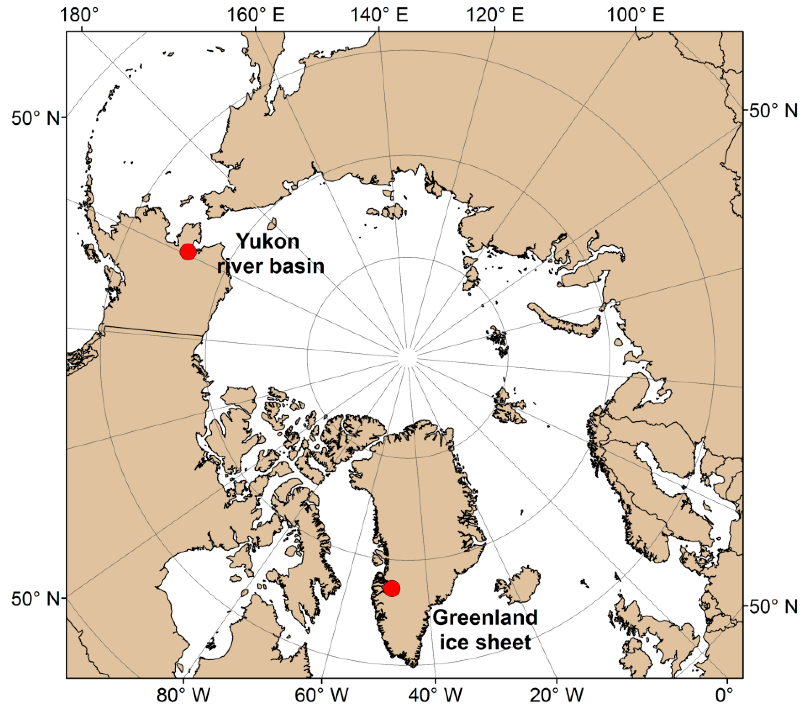
3.2. Study Areas
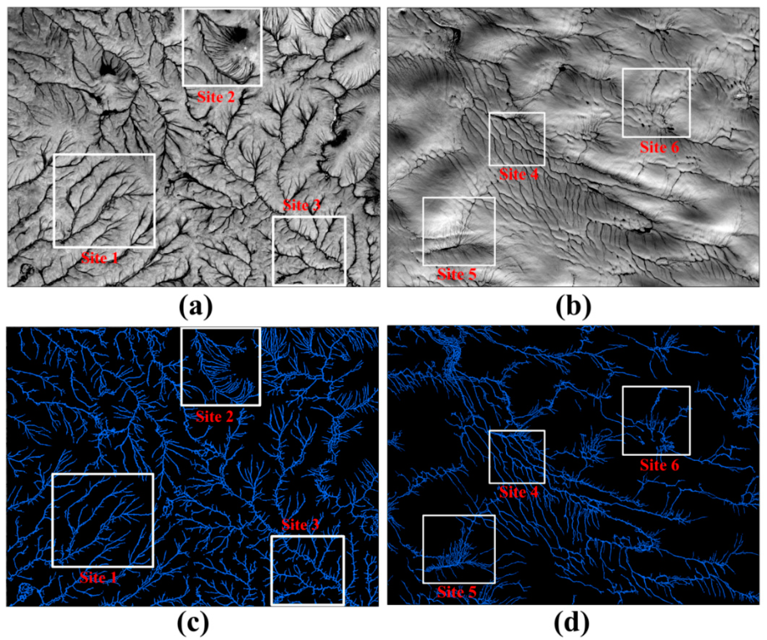
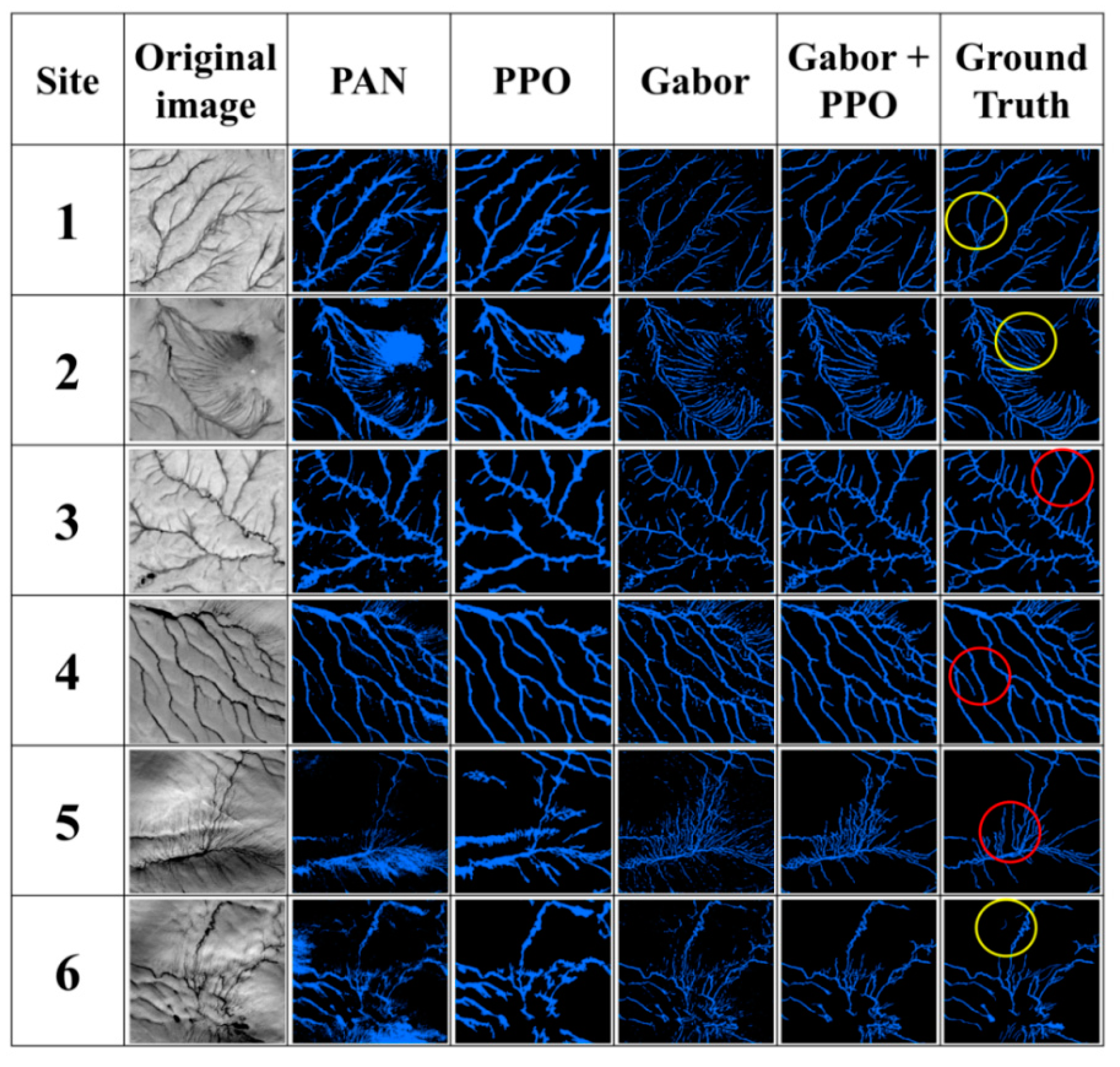
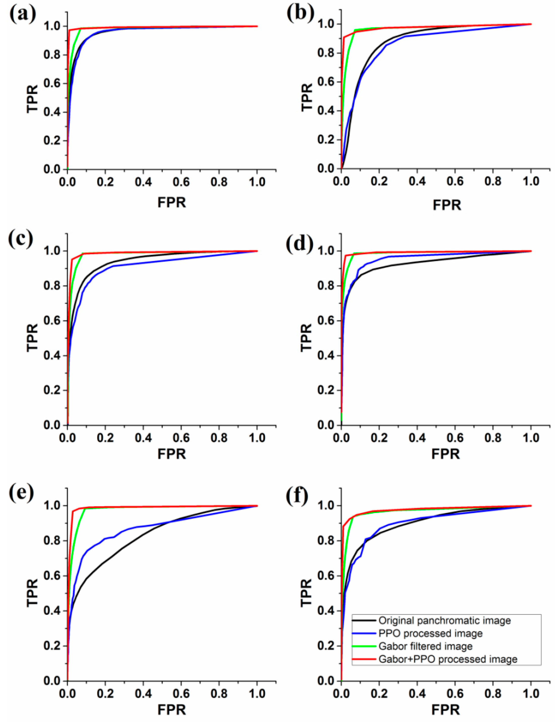
3.3. Detection Accuracy Evaluation


| Image | Site 1 | Site 2 | Site 3 | ||||||
|---|---|---|---|---|---|---|---|---|---|
| Acc | TPR | FPR | Acc | TPR | FPR | Acc | TPR | FPR | |
| Original panchromatic image | 89.92 | 91.33 | 10.27 | 83.65 | 77.67 | 15.31 | 90.59 | 81.16 | 7.68 |
| PPO processed image | 91.19 | 87.84 | 8.35 | 85.09 | 65.93 | 11.57 | 89.68 | 72.17 | 7.11 |
| Gabor filtered image | 95.47 | 76.15 | 1.89 | 94.06 | 82.11 | 3.85 | 94.56 | 74.85 | 1.83 |
| Gabor+PPO processed image | 98.88 | 97.27 | 0.90 | 97.55 | 90.90 | 1.29 | 97.26 | 95.26 | 2.38 |
| Image | Site 4 | Site 5 | Site 6 | ||||||
|---|---|---|---|---|---|---|---|---|---|
| Acc | TPR | FPR | Acc | TPR | FPR | Acc | TPR | FPR | |
| Original panchromatic image | 92.09 | 79.83 | 5.48 | 88.57 | 56.08 | 8.46 | 85.67 | 80.51 | 13.86 |
| PPO processed image | 92.58 | 78.59 | 4.64 | 88.23 | 74.36 | 10.51 | 88.29 | 71.21 | 10.16 |
| Gabor filtered image | 95.08 | 94.19 | 4.74 | 93.47 | 90.83 | 6.29 | 95.23 | 85.96 | 3.93 |
| Gabor+PPO processed image | 97.77 | 97.48 | 2.17 | 97.18 | 96.82 | 2.78 | 98.09 | 88.24 | 1.02 |
3.4. Impacts of Global Thresholding

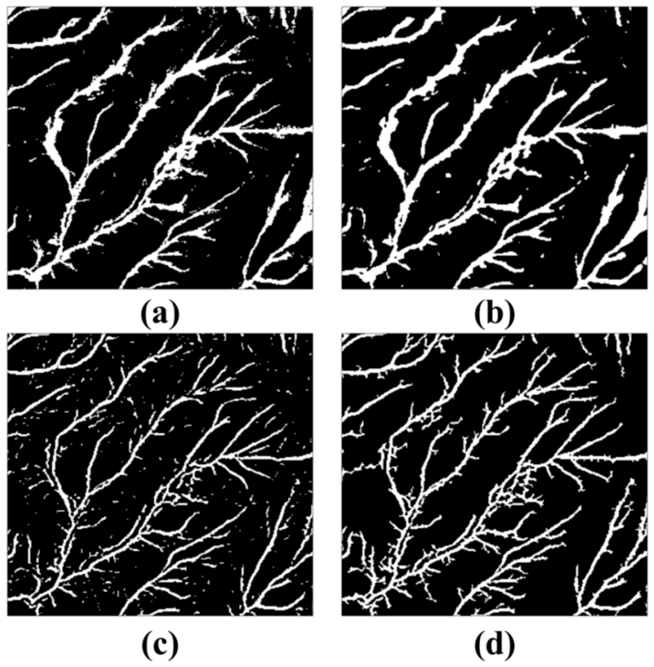
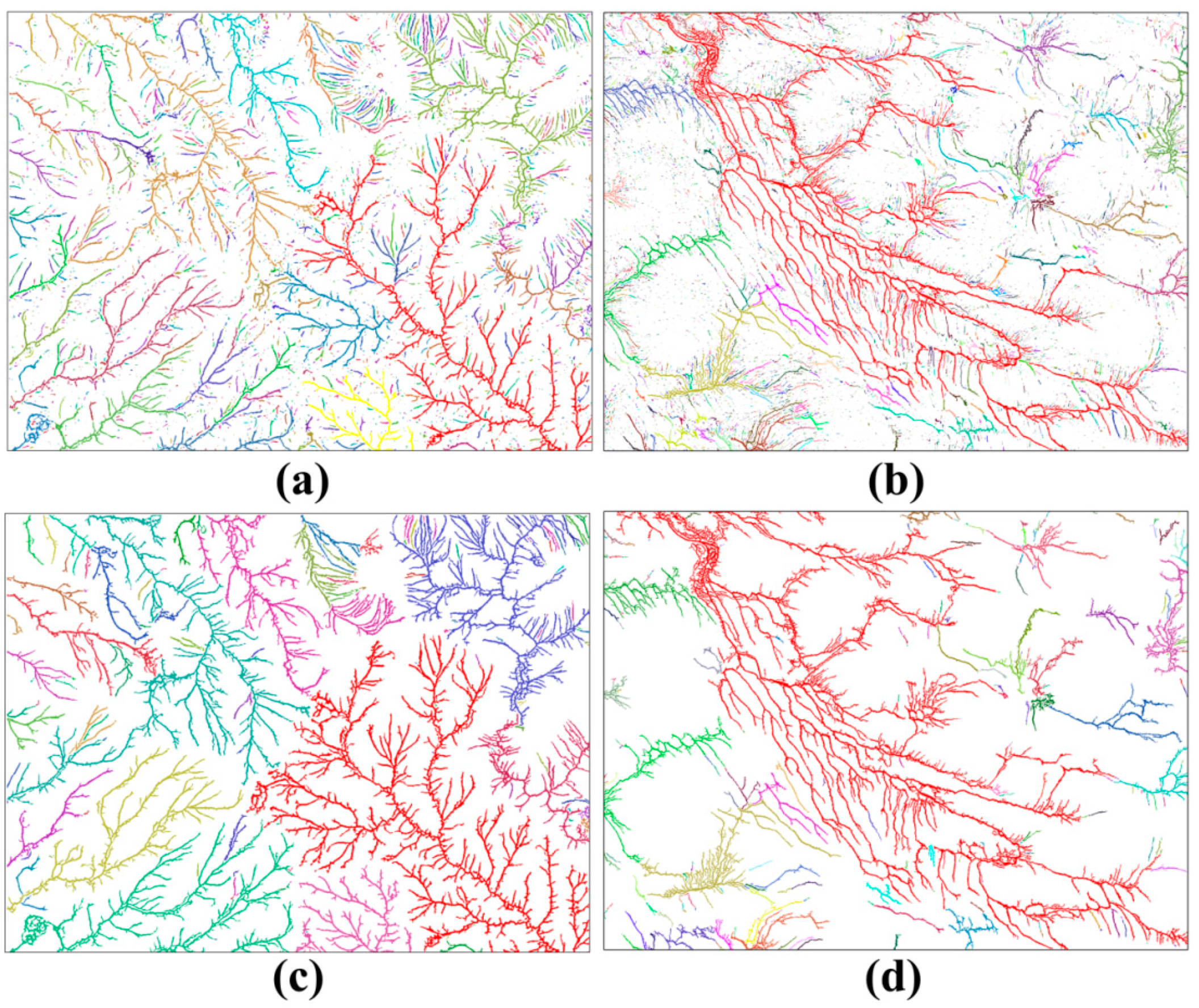
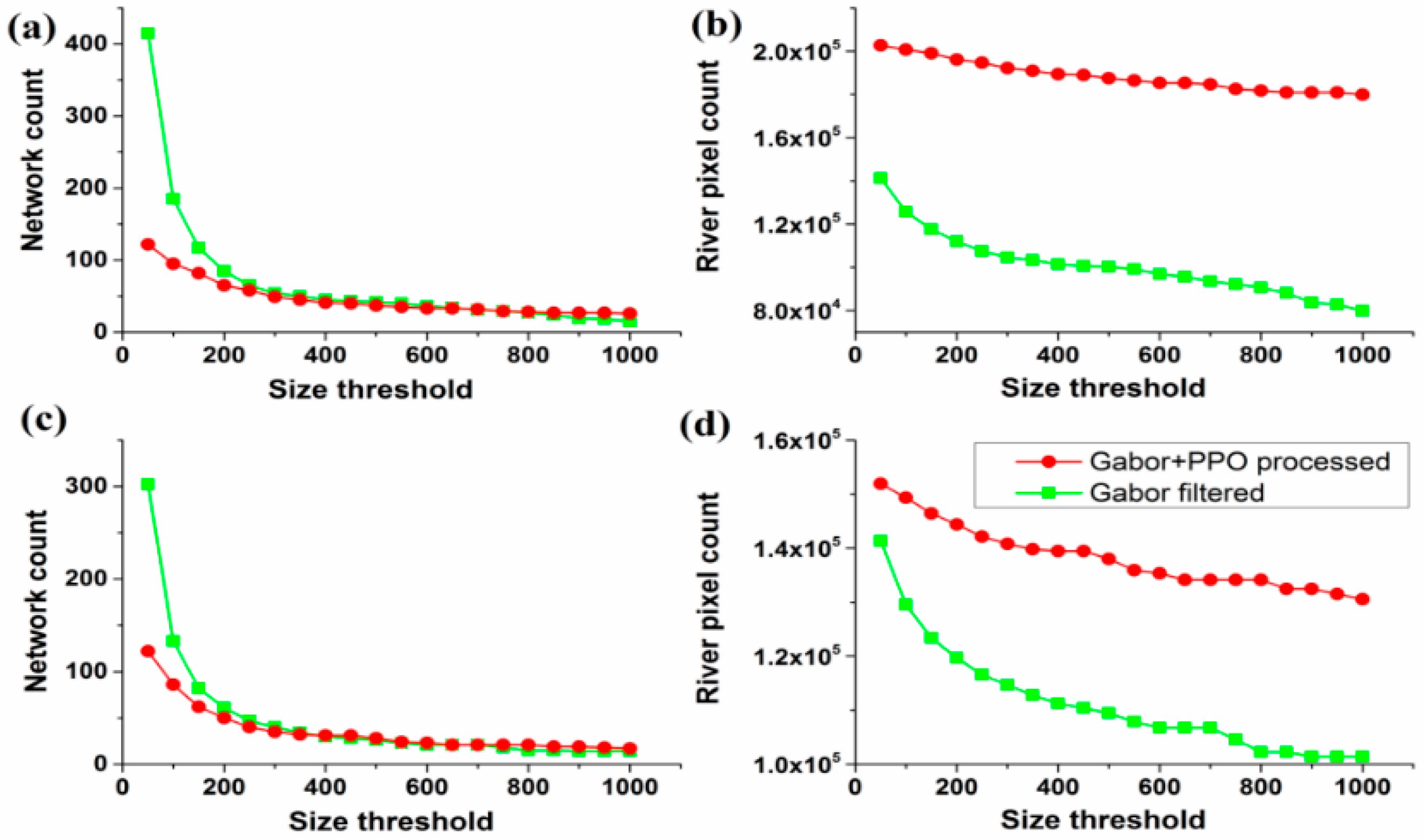
3.5. River Network Continuity Evaluation

| Study Area | Image | Network Count | River Pixel Count | Average Pixel Count per River Network |
|---|---|---|---|---|
| Yukon Basin | Gabor filtered | 5548 | 179,009 | 32 |
| Gabor+PPO processed | 251 | 204,189 | 814 | |
| Greenland Ice Sheet | Gabor filtered | 12,303 | 201,308 | 16 |
| Gabor+PPO processed | 357 | 154,695 | 433 |

4. Discussion and Conclusion
Acknowledgements
Author Contributions
Conflicts of Interest
References
- Vörösmarty, C.J.; Fekete, B.M.; Meybeck, M.; Lammers, R.B. Global system of rivers: Its role in organizing continental land mass and defining land-to-ocean linkages. Glob. Biogeochem. Cycles 2000, 14, 599–621. [Google Scholar] [CrossRef]
- Rosgen, D.L. A classification of natural rivers. CATENA 1994, 22, 169–199. [Google Scholar] [CrossRef]
- Downing, J.A.; Cole, J.J.; Duarte, C.M.; Middelburg, J.J.; Melack, J.M.; Prairie, Y.T.; Kortelainen, P.; Striegl, R.G.; McDowell, W.H.; Tranvik, L.J. Global abundance and size distribution of streams and rivers. Inland Waters 2012, 2, 229–236. [Google Scholar] [CrossRef]
- Yang, K.; Smith, L.C. Supraglacial streams on the greenland ice sheet delineated from combined spectral-shape information in high-resolution satellite imagery. IEEE Geosci. Remote Sens. Lett. 2013, 10, 801–805. [Google Scholar] [CrossRef]
- Mason, D.C.; Scott, T.R.; Wang, H. Extraction of tidal channel networks from airborne scanning laser altimetry. ISPRS J. Photogramm. Remote Sens. 2006, 61, 67–83. [Google Scholar] [CrossRef]
- Trigg, M.A.; Bates, P.D.; Wilson, M.D.; Schumann, G.; Baugh, C. Floodplain channel morphology and networks of the middle amazon river. Water Resour. Res. 2012, 48, W10504. [Google Scholar] [CrossRef]
- Alsdorf, D.E.; Rodriguez, E.; Lettenmaier, D.P. Measuring surface water from space. Rev. Geophys. 2007, 45. [Google Scholar] [CrossRef]
- Zhang, Y. A method for continuous extraction of multispectrally classified urban rivers. Photogramm. Eng. Remote Sens. 2000, 66, 991–999. [Google Scholar]
- McFeeters, S.K. The use of the normalized difference water index (NDWI) in the delineation of open water features. Int. J. Remote Sens. 1996, 17, 1425–1432. [Google Scholar] [CrossRef]
- Shao, Y.; Guo, B.; Hu, X.; Di, L. Application of a fast linear feature detector to road extraction from remotely sensed imagery. IEEE J. Sel. Topics Appl. Earth Observ. Remote Sens. 2011, 4, 626–631. [Google Scholar] [CrossRef]
- Fraz, M.M.; Remagnino, P.; Hoppe, A.; Uyyanonvara, B.; Rudnicka, A.R.; Owen, C.G.; Barman, S.A. Blood vessel segmentation methodologies in retinal images—A survey. Comput. Methods Programs. Biomed. 2012, 108, 407–433. [Google Scholar] [CrossRef] [PubMed]
- Quackenbush, L.J. A review of techniques for extracting linear features from imagery. Photogramm. Eng. Remote Sens. 2004, 70, 1383–1392. [Google Scholar] [CrossRef]
- Ding, X.; Li, X. Monitoring of the water-area variations of lake dongting in China with envisat ASAR images. Int. J. Appl. Earth Obs. Geoinf. 2011, 13, 894–901. [Google Scholar] [CrossRef]
- Ding, X.; Li, X. Shoreline movement monitoring based on SAR images in Shanghai, China. Int. J. Remote Sens. 2014, 35, 3994–4008. [Google Scholar] [CrossRef]
- Ding, X.; Nunziata, F.; Li, X.; Migliaccio, M. Performance analysis and validation of waterline extraction approaches using single- and dual-polarimetric SAR data. IEEE J. Sel. Top. Appl. Earth Observ. Remote Sens. 2015, 8, 1019–1027. [Google Scholar] [CrossRef]
- Liu, Z.; Khan, U.; Sharma, A. A new method for verification of delineated channel networks. Water Resour. Res. 2014, 50, 2164–2175. [Google Scholar] [CrossRef]
- Andreadis, K.M.; Schumann, G.J.P.; Pavelsky, T. A simple global river bankfull width and depth database. Water Resour. Res. 2013, 49, 7164–7168. [Google Scholar] [CrossRef]
- Lehner, B.; Grill, G. Global river hydrography and network routing: Baseline data and new approaches to study the world’s large river systems. Hydrol. Process. 2013, 27, 2171–2186. [Google Scholar] [CrossRef]
- Pavelsky, T.M.; Durand, M.T.; Andreadis, K.M.; Edward Beighley, R.; Paiva, R.C.D.; Allen, G.H.; Miller, Z.F. Assessing the potential global extent of SWOT river discharge observations. J. Hydrol. 2014, 519, 1516–1525. [Google Scholar] [CrossRef]
- Li, J.; Wong, D.W.S. Effects of DEM sources on hydrologic applications. Comput. Environ. Urban Syst. 2010, 34, 251–261. [Google Scholar] [CrossRef]
- Li, S.; MacMillan, R.A.; Lobb, D.A.; McConkey, B.G.; Moulin, A.; Fraser, W.R. Lidar DEM error analyses and topographic depression identification in a hummocky landscape in the prairie region of Canada. Geomorphology 2011, 129, 263–275. [Google Scholar] [CrossRef]
- Kenward, T.; Lettenmaier, D.P.; Wood, E.F.; Fielding, E. Effects of digital elevation model accuracy on hydrologic predictions. Remote Sens. Environ. 2000, 74, 432–444. [Google Scholar] [CrossRef]
- Rinne, E.J.; Shepherd, A.; Palmer, S.; van den Broeke, M.R.; Muir, A.; Ettema, J.; Wingham, D. On the recent elevation changes at the Flade Isblink Ice Cap, Northern Greenland. J. Geophys. Res. Earth 2011, 116. [Google Scholar] [CrossRef]
- Schenk, T.; Csatho, B.; van der Veen, C.; McCormick, D. Fusion of multi-sensor surface elevation data for improved characterization of rapidly changing outlet glaciers in Greenland. Remote Sens. Environ. 2014, 149, 239–251. [Google Scholar] [CrossRef]
- Allen, G.H.; Barnes, J.B.; Pavelsky, T.M.; Kirby, E. Lithologic and tectonic controls on bedrock channel form at the northwest Himalayan front. J. Geophys. Res. -Earth 2013, 118, 1806–1825. [Google Scholar] [CrossRef]
- Lampkin, D.J.; Amador, N.; Parizek, B.R.; Farness, K.; Jezek, K. Drainage from water-filled crevasses along the margins of Jakobshavn Isbræ: A potential catalyst for catchment expansion. J. Geophys. Res. -Earth 2013, 118, 795–813. [Google Scholar] [CrossRef]
- Fairfield, J.; Leymarie, P. Drainage networks from grid digital elevation models. Water Resour. Res. 1991, 27, 709–717. [Google Scholar] [CrossRef]
- Pavelsky, T.M.; Smith, L.C. Rivwidth: A software tool for the calculation of river widths from remotely sensed imagery. IEEE Geosci. Remote Sens. Lett. 2008, 5, 70–73. [Google Scholar] [CrossRef]
- Lawford, R.; Strauch, A.; Toll, D.; Fekete, B.; Cripe, D. Earth observations for global water security. Curr. Opin. Environ. Sustain. 2013, 5, 633–643. [Google Scholar] [CrossRef]
- Brierley, G.; Fryirs, K.; Cullum, C.; Tadaki, M.; Huang, H.Q.; Blue, B. Reading the landscape: Integrating the theory and practice of geomorphology to develop place-based understandings of river systems. Prog. Phys. Geogr. 2013, 37. [Google Scholar] [CrossRef]
- Mertes, L.A.K. Remote sensing of riverine landscapes. Freshw. Biol. 2002, 47, 799–816. [Google Scholar] [CrossRef]
- Marcus, W.A.; Fonstad, M.A. Remote sensing of rivers: The emergence of a subdiscipline in the river sciences. Earth Surf. Proc. Land. 2010, 35, 1867–1872. [Google Scholar] [CrossRef]
- Benstead, J.P.; Leigh, D.S. An expanded role for river networks. Nat. Geosci. 2012, 5, 678–679. [Google Scholar] [CrossRef]
- Dillabaugh, C.R.; Niemann, K.O.; Richardson, D.E. Semi-automated extraction of rivers from digital imagery. Geoinformatica 2002, 6, 263–284. [Google Scholar] [CrossRef]
- Pai, N.; Saraswat, D. A geospatial tool for delineating streambanks. Environ. Modell. Softw. 2013, 40, 151–159. [Google Scholar] [CrossRef]
- Lau, T.; Franklin, W.R. River network completion without height samples using geometry-based induced terrain. Cartogr. Geogr. Inf. Sci. 2013, 40, 316–325. [Google Scholar] [CrossRef]
- Klemenjak, S.; Waske, B.; Valero, S.; Chanussot, J. Automatic detection of rivers in high-resolution SAR data. IEEE J. Sel. Topics Appl. Earth Observ. Remote Sens. 2012, 5, 1364–1372. [Google Scholar] [CrossRef]
- Güneralp, İ.; Filippi, A.M.; Hales, B.U. River-flow boundary delineation from digital aerial photography and ancillary images using support vector machines. Gisci. Remote Sens. 2013, 50, 1–25. [Google Scholar]
- Jiang, H.; Feng, M.; Zhu, Y.; Lu, N.; Huang, J.; Xiao, T. An automated method for extracting rivers and lakes from Landsat imagery. Remote Sens. 2014, 6, 5067–5089. [Google Scholar] [CrossRef]
- Yang, K.; Li, M.; Liu, Y.; Cheng, L.; Duan, Y.; Zhou, M. River delineation from remotely sensed imagery using a multi-scale classification approach. IEEE J. Sel. Top. Appl. Earth Observ. Remote Sens. 2014, 7, 4726–4737. [Google Scholar] [CrossRef]
- Welikala, R.A.; Dehmeshki, J.; Hoppe, A.; Tah, V.; Mann, S.; Williamson, T.H.; Barman, S.A. Automated detection of proliferative diabetic retinopathy using a modified line operator and dual classification. Comput. Methods. Prog. Biomed. 2014, 114, 247–261. [Google Scholar] [CrossRef] [PubMed]
- Pizer, S.M.; Amburn, E.P.; Austin, J.D.; Cromartie, R.; Geselowitz, A.; Greer, T.; ter Haar Romeny, B.; Zimmerman, J.B.; Zuiderveld, K. Adaptive histogram equalization and its variations. Comput. Vis. Graph. Image. Process. 1987, 39, 355–368. [Google Scholar] [CrossRef]
- Zhou, G.; Cui, Y.; Chen, Y.; Yang, J.; Rashvand, H.; Yamaguchi, Y. Linear feature detection in polarimetric SAR images. IEEE Trans. Geosci. Remote Sens. 2011, 49, 1453–1463. [Google Scholar] [CrossRef]
- Oliveira, H.; Correia, P.L. Automatic road crack detection and characterization. IEEE Trans. Intell. Transp. Syst. 2013, 14, 155–168. [Google Scholar] [CrossRef]
- Chaudhuri, S.; Chatterjee, S.; Katz, N.; Nelson, M.; Goldbaum, M. Detection of blood vessels in retinal images using two-dimensional matched filters. IEEE Trans. Med. Imag. 1989, 8, 263–269. [Google Scholar] [CrossRef] [PubMed]
- Zhang, B.; Zhang, L.; Zhang, L.; Karray, F. Retinal vessel extraction by matched filter with first-order derivative of gaussian. Comput. Biol. Med. 2010, 40, 438–445. [Google Scholar] [CrossRef] [PubMed]
- Liu, J.; Feng, D. Two-dimensional multi-pixel anisotropic gaussian filter for edge-line segment (ELS) detection. Image Vis. Comput. 2014, 32, 37–53. [Google Scholar] [CrossRef]
- Rangayyan, R.M.; Ayres, F.J.; Oloumi, F.; Oloumi, F.; Eshghzadeh-Zanjani, P. Detection of blood vessels in the retina with multiscale Gabor filters. J. Electron. Imaging 2008, 17. [Google Scholar] [CrossRef]
- Lau, T.; Franklin, W.R. Completing fragmentary river networks via induced terrain. Cartogr. Geogr. Inf. Sci. 2011, 38, 162–174. [Google Scholar]
- Yang, K.; Li, M.; Liu, Y.; Jiang, C. Multi-points fast marching: A novel method for road extraction. In Proceedings of the 2010 18th International Conference on Geoinformatics 2010, Beijing, China, 18–20 June 2010; pp. 1–5.
- Heijmans, H.; Buckley, M.; Talbot, H. Path openings and closings. J. Math. Imaging Vis. 2005, 22, 107–119. [Google Scholar] [CrossRef]
- Valero, S.; Chanussot, J.; Benediktsson, J.A.; Talbot, H.; Waske, B. Advanced directional mathematical morphology for the detection of the road network in very high resolution remote sensing images. Pattern Recogn. Lett. 2010, 31, 1120–1127. [Google Scholar] [CrossRef] [Green Version]
- Morard, V.; Dokladal, P.; Decenciere, E. Parsimonious path openings and closings. IEEE Trans. Image Process. 2014, 23, 1543–1555. [Google Scholar] [CrossRef] [PubMed]
- Fawcett, T. An introduction to ROC analysis. Pattern Recogn. Lett. 2006, 27, 861–874. [Google Scholar] [CrossRef]
- Nijssen, B.; O’Donnell, G.M.; Lettenmaier, D.P.; Lohmann, D.; Wood, E.F. Predicting the discharge of global rivers. J. Clim. 2001, 14, 3307–3323. [Google Scholar] [CrossRef]
© 2015 by the authors; licensee MDPI, Basel, Switzerland. This article is an open access article distributed under the terms and conditions of the Creative Commons Attribution license (http://creativecommons.org/licenses/by/4.0/).
Share and Cite
Yang, K.; Li, M.; Liu, Y.; Cheng, L.; Huang, Q.; Chen, Y. River Detection in Remotely Sensed Imagery Using Gabor Filtering and Path Opening. Remote Sens. 2015, 7, 8779-8802. https://doi.org/10.3390/rs70708779
Yang K, Li M, Liu Y, Cheng L, Huang Q, Chen Y. River Detection in Remotely Sensed Imagery Using Gabor Filtering and Path Opening. Remote Sensing. 2015; 7(7):8779-8802. https://doi.org/10.3390/rs70708779
Chicago/Turabian StyleYang, Kang, Manchun Li, Yongxue Liu, Liang Cheng, Qiuhao Huang, and Yangming Chen. 2015. "River Detection in Remotely Sensed Imagery Using Gabor Filtering and Path Opening" Remote Sensing 7, no. 7: 8779-8802. https://doi.org/10.3390/rs70708779