Detecting Change Dates from Dense Satellite Time Series Using a Sub-Annual Change Detection Algorithm

Abstract

Multi-temporal satellite images are available at very high revisit frequency, allowing the characterization of land-cover transitions and trajectories in greater detail. However, most change detection methods aim to capture a snapshot of land cover, for instance on an annual scale, which do not describe changes that occurred between the annual time points. In this study, we present a sub-annual change detection (SCD) approach to detect change dates from dense satellite time series. SCD estimates change dates by analyzing differences between two consecutive annual segments in two steps. To validate the proposed method, SCD was applied to real and simulated time series of MODIS 16-day NDVI from 2000 to 2012 for MODIS tile h11v05 and a sub-area in southeast Ohio, USA. The results show that SCD can successfully detect from dense time series the dates of changes representing land-cover transitions among various vegetated land covers. In addition, SCD can achieve comparable accuracy on the date of abrupt land-cover changes for the real time series tested in the study area when compared with the trend and seasonal changes identified by a Breaks for Additive Seasonal and Trend (BFAST) method. Future effort will be given to apply the proposed approach to various remotely sensed time series for other areas with extreme climates.

1. Introduction

Land-use and land-cover change by modification of the Earth’s land surface over time highlights interactions between the human and physical environment [1,2]. In order to understand the environmental and social impacts of the changes and project future changes and potential impacts, it is essential to quantify the intensity of land-cover changes over time. Remote sensing has become the preferred method for detecting land-cover changes over time due to its advantages of consistent and repeatable procedures [3,4]. Remotely sensed data provides continuous, quantitative, and spatially explicit observations, which can characterize a variety of land-cover types and transitions between different types [3,4].

Abrupt land-cover change (shortened to land-cover change hereafter) refers to the conversion of land-cover from one class (e.g., forest) to another class (e.g., grassland). Land-cover change over a period of time, or land-cover trajectory, can be constructed from satellite images acquired at multiple time points [5,6,7]. With the recent advances in earth observations, dense time series of satellite images become widely available, such as MODIS (Moderate Resolution Imaging Spectroradiometer) data, which allows researchers to address land-cover trajectories in a continuous time frame. Continuous mapping, moving beyond the annual land-cover “snapshot” at a discrete time point, can provide more complete information at each available time point than the traditional annual map. With the improved capacity of multi-temporal satellite data, more and more studies have put effort to analyze long time series to characterize land-cover change trajectories [6,8,9]. Kaufmann and Seto [8] proposed a method based on panel econometric techniques to determine the time points of land-cover change in a time series of Landsat Thematic Mapper (TM) images. Changes were identified by comparing a pixel’s digital number (DN) values to those of land-cover changes predicted from regressions for each possible date. This method provides an approach different from conventional change detection but it was not designed to detect changes from high-resolution time series. Recently, a regression-based approach was developed to detect trajectories of forest disturbance and recovery using yearly time series images [5,9]. This approach fits a sequence of straight lines to the observed spectral profiles extracted and eliminates noise. The change detection methods developed at yearly resolution, however, cannot be directly applied to time series data at higher temporal resolution (e.g., monthly) for most vegetated land covers due to the confusion with seasonal variations in vegetation phenology (except for vegetation with little seasonal variation), and thus they are not able to capture accurate change points at scales less than one year.

The major challenge for detecting changes in dense satellite time series is to distinguish land-cover change from seasonal phenological variation. Methods have been developed for change point detection in statistics by identifying the points where significant differences between probability distributions are generated over different intervals [10] and in signal processing by data segmentation techniques [11,12,13]. These methods were developed for use with signal data and are not well adapted to image time series and land-cover changes which have fewer observations per cycle and smoother transitions at change points compared to common signal data. In fact, methods of detecting dates of land-cover change from image time series have been rarely explored. Goodwin and Collett [14] employed dense time series of Landsat images to map the event of fire by detecting the negative outliers relative to the median-smoothed time series. Verbesselt et al. [15] proposed a Breaks for Additive Seasonal and Trend (BFAST) method to analyze the dynamics of time series using the MODIS 16-day NDVI (normalized difference of vegetation index) product from 2000 to 2008. They demonstrate that time series can be decomposed into trend, seasonal, and remainder components and the time and number of changes can be detected at high temporal resolution (i.e., 16 days). In a recent study, Jamali et al. [16] proposed a user-friendly program, Detecting Breakpoints and Estimating Segments in Trend (DBEST), to characterize the time and magnitude of changes in vegetation trends from NDVI time series using a segmentation algorithm. They tested the program with bimonthly NDVI time series at 8-km spatial resolution.

The objective of this study is to develop a new approach for detecting change points of abrupt land-cover changes at sub-annual scale using dense time series of satellite observations. We propose a sub-annual change detection approach to detect the dates of change (change dates, henceforth) and account for seasonal variations in time series of image data. Using reference and simulated time series of MODIS 16-day NDVI from 2000 to 2012, we assessed the performance of the proposed method on the accuracy of change date detection and compared the results with the trend and seasonal changes detected by the BFAST [15] method.

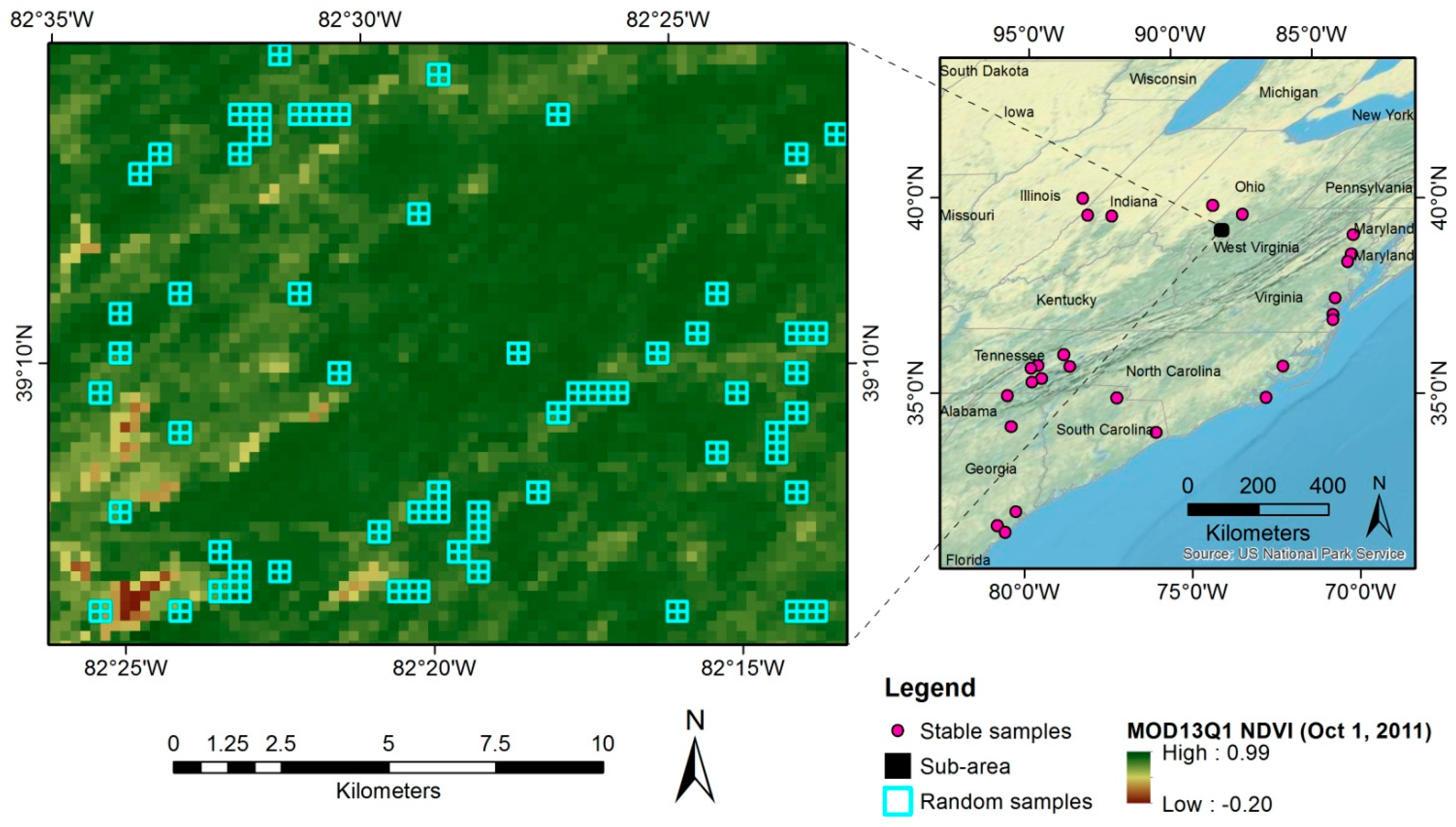
Figure 1. The locations of stable samples (no land-cover change), sub-area, and random samples in the sub-area. The image renders the MOD13Q1 NDVI acquired on 1 October 2011 shown in the extent of the sub-area.

Figure 1. The locations of stable samples (no land-cover change), sub-area, and random samples in the sub-area. The image renders the MOD13Q1 NDVI acquired on 1 October 2011 shown in the extent of the sub-area.

2. MODIS NDVI Time Series

The change date detection method was developed for dense time series of remotely sensed data. We demonstrate the method on a 13-year time series of MODIS NDVI 16-day L3 data at 250-meter resolution (MOD13Q1), which were acquired for the tile h11v05 (Figure 1) from February 2000 to April 2012. Each time series consists of a total of 281 observations, which were placed sequentially in the time domain of each pixel. The MODIS NDVI products are computed from atmospherically corrected, bi-directional surface reflectances that have been masked for water, clouds, heavy aerosols, and cloud shadows. Documentation of MOD13Q1, the processing algorithm, and quality assurance system can be found at NASA’s MODIS website [17]. The quality assurance (QA) data in the product are provided for each pixel based on examination and accuracy estimation using input and output data, system noise, and algorithmic specifications [17,18]. The advantages of using NDVI for change date detection is that land-cover changes may be emphasized by NDVI compared to the spectral values [19,20].

3. Method

Our method analyzes time series at different temporal scales to detect change points within a time series. The change points represent abrupt land-cover change, which is different from seasonal variation. A time series was first pre-processed with simple smoothing techniques to remove noise and obtain an uninterrupted data stream. Then statistical methods are applied to the time series to detect change points. We use the time series of MODIS NDVI data as an example, although the method is not limited to MODIS data. 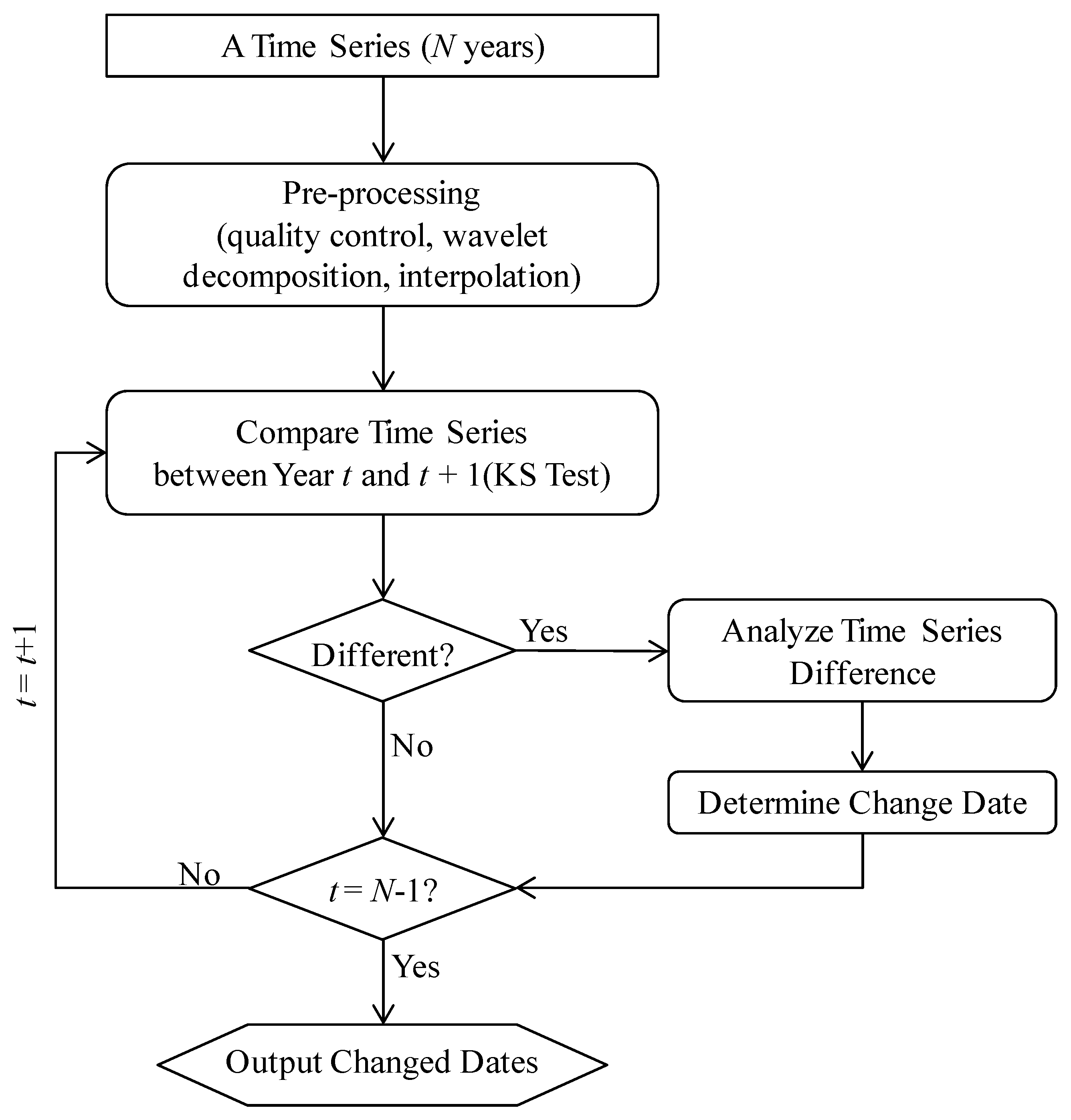Figure 2 illustrates the flow of the proposed method, which is detailed in the following sections.

Figure 2. Flow chart of the proposed method for detecting change date in a time series.

Figure 2. Flow chart of the proposed method for detecting change date in a time series.

3.1. Pre-Processing

Noise in a time series is brought about by cloud contamination and other factors such as snow or device malfunction. Pre-processing is necessary to reduce this noise because it may conceal actual trends in a time series. We employed the QA data to remove low quality observations by retaining the time points in a time series flagged as “good quality” (values computed from a day with high quality without the nadir view requirement; [17]). In addition to the QA data, a test for sudden drops was conducted to retain good quality values throughout the time series [21]. The application of this test ensures data quality, especially when QA information is imperfect or missing. The test searches forward and rejects points that have both low value and follow a value, which is greater than 20% of the difference between the low value and its previous high value. 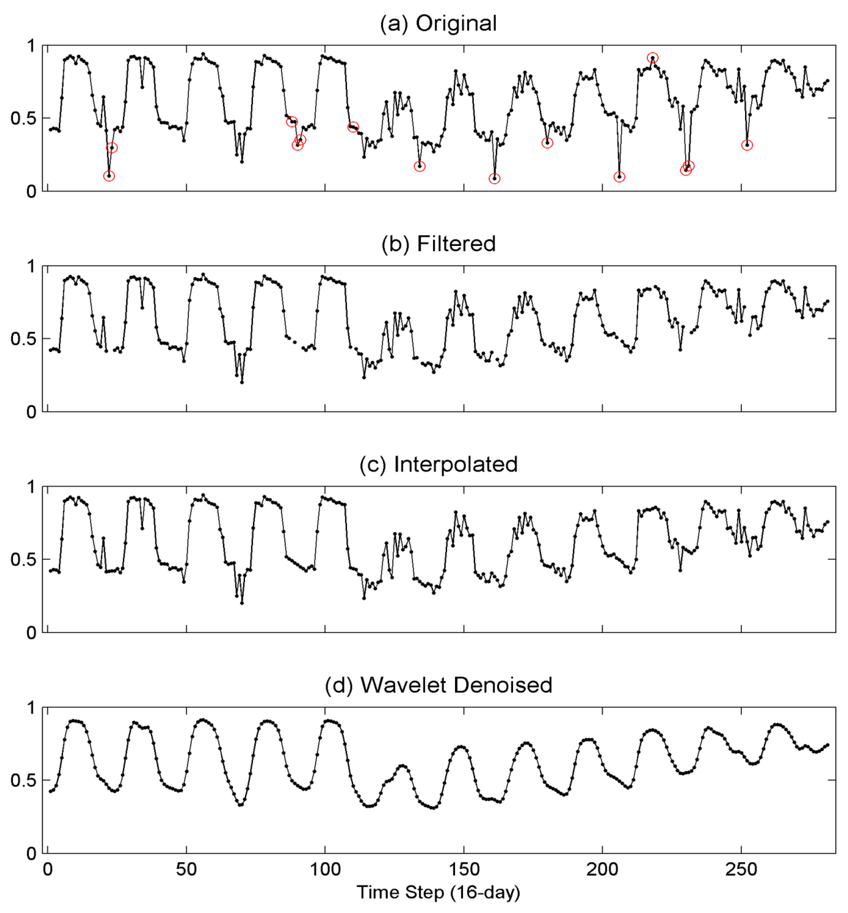This technique is designed to record the process of transitioning from cloudy to clear sky conditions [21]. It can preserve the values recording the gradual process of re-growth from fire or drought, which were not represented by sudden falls and rises (sudden drops) in NDVI. By utilizing the QA data and implementing the test for sudden drops, the observation points contaminated by various noises were detected and discarded from the time series. The values at those points were then filled by implementing a simple three-point moving average interpolation (Figure 3a–c).

Figure 3. Pre-processing procedures implemented on a NDVI time series: (a) original time series (the red circles mark the time points that are filtered based on QA data); (b) time series retained after filtering based on QA data; (c) time series with linear interpolation on filtered points; and (d) time series attained after wavelet decomposition.

Figure 3. Pre-processing procedures implemented on a NDVI time series: (a) original time series (the red circles mark the time points that are filtered based on QA data); (b) time series retained after filtering based on QA data; (c) time series with linear interpolation on filtered points; and (d) time series attained after wavelet decomposition.

Next, we utilized a wavelet decomposition technique to reduce high frequency or random noise and smooth the time series while preserving local details [22]. A four-level Haar wavelet decomposition [23] was applied to decompose the time series into four components, each with a set of approximation parameters at different levels. The time series was smoothed by being reconstructed from the low frequency component at the fourth level. Figure 3d shows the reconstructed time series, which greatly reduced noise due to cloudy conditions or random noise compared with the original time series (Figure 3a).

3.2. Detecting Change Dates

To detect the points in a time series when land-cover changed, we developed a sub-annual approach that detects changes in two steps. In the first step, annual time series were compared to detect years that have different characteristics from neighboring years. Within those “changed years”, the second step detects the observation points that do not follow seasonal patterns. The two steps were conducted at “year” and “date” levels hierarchically and sequentially. Such a hierarchical approach has been similarly employed in data segmentation techniques [11]; it saves computational cost and shows flexibility by being able to modify results with updated observations. The details for each step are described in the following sections.

3.2.1. Step 1: Detecting Change between Years

The smoothed time series was divided into segments by calendar year such that each segment contained records acquired in one year. One record for every 16-day interval equals 23 observations for the MODIS NDVI time series. The first and the last years did not have 23 records because the observations in the beginning of 2000 and the end of 2012 were unavailable. Between a pair of neighboring years, we conducted a two-sample Kolmogorov–Smirnov (KS) test to determine if the two time series showed different characteristics. The KS test is a non-parametric test with the null hypothesis that the two samples are from the same continuous distribution. The test is a distribution-free test and commonly used to detect structural change in a time series [24,25,26]. The mathematical explanation for the KS test can be found in Massey [27].

The two-sample KS test compares the first and second years in a time series and then moves on to subsequent years. The null hypothesis is valid only when the two time series represent the same land cover because (1) both non-random noise (cloud cover, snow, device malfunction, etc.) and random noise (high frequency noise) were already removed in the pre-processing step; and (2) the annual variability of the NDVI time series was likely to be consistent with homogenous land cover. In other words, if the null hypothesis of the KS test is rejected, the time series of the second year represents a different land cover compared to the first year; otherwise, no land cover changed during the second year. The null hypothesis is rejected based on a predefined significance level, denoted by α. If a change is detected in a year, the algorithm flags it for further analysis in the next step. Otherwise, the KS test moves on to the second and third years.

3.2.2. Step 2: Detecting Change within Years

Step 2 is implemented to detect change points if a year was flagged with change in Step 1; otherwise, this step is skipped. The goal is to find the time point where the NDVI values deviate from the previous part. The procedure compares the time series of a flagged year with the year before and seeks a shift point in deviation. We refer to a point in a time series as a date hereafter, represented by a temporal index in a year. Consider a time series having n observation records each year for m years. Let $\mathit{X}=\left\{X_{i,t}\right\}$ denote the observation value (e.g., NDVI) on date t in year i with $i\in M=\left\{1,2,\mathrm{...},m\right\}$ and $t\in T=\left\{1,2,\mathrm{...},n\right\}$, where n is the number of records in each year (n = 23 for the 16-day NDVI time series). The absolute difference $\mathbf{D}=\left\{D_{i-1,i,t}|i\in M,t\in T\right\}$ is calculated between the two years on each date t as

$${\mathit{D}}_{i-1,i,t}=\left|X_{i-1,t}-X_{i,t}\right|$$

(1)

The change from one land-cover type to another will cause an abrupt shift toward greater value in D on the change date. This jump ought not to occur only on a single date but also on the following days with similar greater deviation. The reason is that a change in land cover is likely low frequency in a certain period of time and distinct from recurrent intra-annual variations. Specifically, suppose year i be flagged in Step 1, the date t* in year i will be determined as the change date if it satisfies two criteria at the same time:

$$\begin{array}{l}\text{i) }{D}_{i-1,i,t\ast -p}<\kappa \text{, }\forall p=1,2,3,\mathrm{...},t\ast -1\\ \text{ii) }{D}_{i-1,i,t\ast +p}>\kappa \text{, }\forall p=0,1,2,\mathrm{...},p*\end{array}$$

(2)

where $\text{κ}$ is a threshold, and p* is the least number of records that show deviation after the change date. We determined p* to be 3, based on some trial and error experiments. The threshold $\kappa$ is calculated by multiplying a scale factor (β) and the maximum of the absolute difference ($D_{\max }$):

$$\text{κ}=\text{β}\cdot D_{\max }$$

(3)

where the value of the scale factor β is determined during the training process.

Once a change date t* is detected in year i, the algorithm returns to the yearly scale and implements Step 1 for the next two consecutive years. In the cases that a change date t* is detected in the year i – 1 of two consecutive years, only the records acquired on dates from t* + 1 to n in years i – 1 and i will be utilized to calculate D and tested against the two criteria in Equation (2).

3.3. Algorithm Training

Two parameters in the proposed algorithm are user-defined: the significance level α for the KS test in Step 1 and the scale factor β for determination of the change date in Step 2. The significance level is usually valued at 0.1, 0.05, or 0.01 [27], while the scale factor is a positive number reasonably smaller than 4. A grid search technique was used to select the values of the two parameters with training samples. The values in the grid search ranged from 0.01 to 0.1 with an incretion of 0.005 for significance level and from 1 to 3 with an incretion of 0.05 for the scale factor. The parameters were determined when the both lowest root mean squared error (RMSE, refer to Section 3.4) for the time of detected change and lowest RMSE for the number of changes were obtained.

3.4. Accuracy Assessment

The accuracy of the proposed method was assessed for two variables: the number of detected changes and the time of a detected change. The latter was measured in units of “step”, with each step equaling 16 days in this study. To measure the difference between estimated values and reference values, root mean squared error (RMSE) and mean signed error (MSE) are calculated for each variable:

$$\mathrm{RMSE}=\sqrt{\frac{1}{n}{\displaystyle \sum _{k=1}^n{\left({\widehat{Y}}_k-Y_k\right)}^2}}$$

(4)

and

$$\mathrm{MSE}=\frac{1}{n}{\displaystyle \sum _{k=1}^n\left({\widehat{Y}}_k-Y_k\right)}$$

(5)

where n is the number of samples and ${\widehat{Y}}_k$ is an estimate of the true value $Y_k$ for the kth sample. Specifically, $Y_k$ and ${\widehat{Y}}_k$ correspond to the true and estimated number of detected changes or the true and estimated time of a detected change. For the time of detected change, only the samples that have changes are used to compute the two indices. Samples that have changes but not detected by the method indicate omission errors, which were calculated as a percentage relative to the total number of time series tested. Similarly, stable time series that were labeled as changed are regarded as false changes indicating commission errors.

4. Validation

4.1. Validation Datasets

We used two datasets of time series to test the accuracy of change date detection: one representing portions of International Geosphere–Biosphere Program (IGBP) [28] land-cover classes and the other a set of randomly selected pixels in the study area. Validation of multi-temporal change detection methods requires independent reference data for a broad range of potential changes and thus is often not straightforward [15]. We extracted MODIS NDVI time series for known stable IGBP land-cover classes with which changes were simulated. The simulated time series is capable of representing a variety of land-cover changes. The second dataset was obtained independently; real NDVI time series were obtained for pixels, which were randomly selected within the study area. The reference change dates were identified from Landsat TM images that are available during the time period. In the next two sections, we describe the two datasets for validation.

4.1.1. IGBP Stable Samples and Simulated Changes

We acquired the reference land-cover labels for 402 pixels in MODIS tile h11v05 from the Land Cover and Surface Climate Group at Boston University. All pixels represent stable land cover from 2000 to 2012. The reference dataset were derived from and systematically maintained by manual interpretation of Landsat Thematic Mapper (TM) data, Landsat 7 data, orthorectified Geocover 2000 imagery, augmented by ancillary map data and Google Earth^© imagery [29,30]. The dataset includes six IGBP land-cover classes (Table 1).

Table 1. IGBP (International Geosphere–Biosphere Program) land-cover classes and definitions (modified from [30]).

Index	IGBP Land-Cover Class	Definition
1	Deciduous broadleaf forest	Lands dominated by woody vegetation with a percent cover >60% and height exceeding 2 m.
2	Mixed forest	Lands dominated by trees with a percent cover >60% and height exceeding 2 m. Consists of tree communities with interspersed mixtures or mosaics of evergreen needleleaf, evergreen broadleaf, deciduous needleleaf, and deciduous broadleaf forest, none of which exceeds 60% of landscape.
3	Woody savannas	Lands with herbaceous and other understory systems, and with forest canopy cover between 30% and 60%. The forest cover height exceeds 2 m.
4	Permanent wetlands	Lands with a permanent mixture of water and herbaceous or woody vegetation. The vegetation can be present either in salt, brackish, or fresh water.
5	Croplands	Lands covered with temporary crops followed by harvest and a bare soil period (e.g., single and multiple cropping systems). Note that perennial woody crops will be classified as the appropriate forest or shrub land-cover type.
6	Croplands/natural vegetation mosaic	Lands with a mosaic of croplands, forests, shrubland, and grasslands in which no one component comprises more than 60% of the landscape.

Table 1. IGBP (International Geosphere–Biosphere Program) land-cover classes and definitions (modified from [30]).

Index	IGBP Land-Cover Class	Definition
1	Deciduous broadleaf forest	Lands dominated by woody vegetation with a percent cover >60% and height exceeding 2 m.
2	Mixed forest	Lands dominated by trees with a percent cover >60% and height exceeding 2 m. Consists of tree communities with interspersed mixtures or mosaics of evergreen needleleaf, evergreen broadleaf, deciduous needleleaf, and deciduous broadleaf forest, none of which exceeds 60% of landscape.
3	Woody savannas	Lands with herbaceous and other understory systems, and with forest canopy cover between 30% and 60%. The forest cover height exceeds 2 m.
4	Permanent wetlands	Lands with a permanent mixture of water and herbaceous or woody vegetation. The vegetation can be present either in salt, brackish, or fresh water.
5	Croplands	Lands covered with temporary crops followed by harvest and a bare soil period (e.g., single and multiple cropping systems). Note that perennial woody crops will be classified as the appropriate forest or shrub land-cover type.
6	Croplands/natural vegetation mosaic	Lands with a mosaic of croplands, forests, shrubland, and grasslands in which no one component comprises more than 60% of the landscape.

Based on the six stable land-cover classes, we simulated land-cover changes by combining truncated time series that represent stable land cover. Specifically, let $\mathit{w}=\left\{w_j|j=1,\mathrm{...},C\right\}$ denote the set of land-cover classes and $\left(Y_1^{w_j},Y_2^{w_j},\mathrm{...},Y_n^{w_j}\right)$ denote a time series of class w_j with n observations in a time period of T. A change from class w₁ to class w₂ may be simulated as

$$\left(Y_1^{w_1},\mathrm{...},Y_{t*-1}^{w_1},Y_{t*}^{w_2},Y_{t*+1}^{w_2},\mathrm{...},Y_n^{w_2}\right),$$

(6)

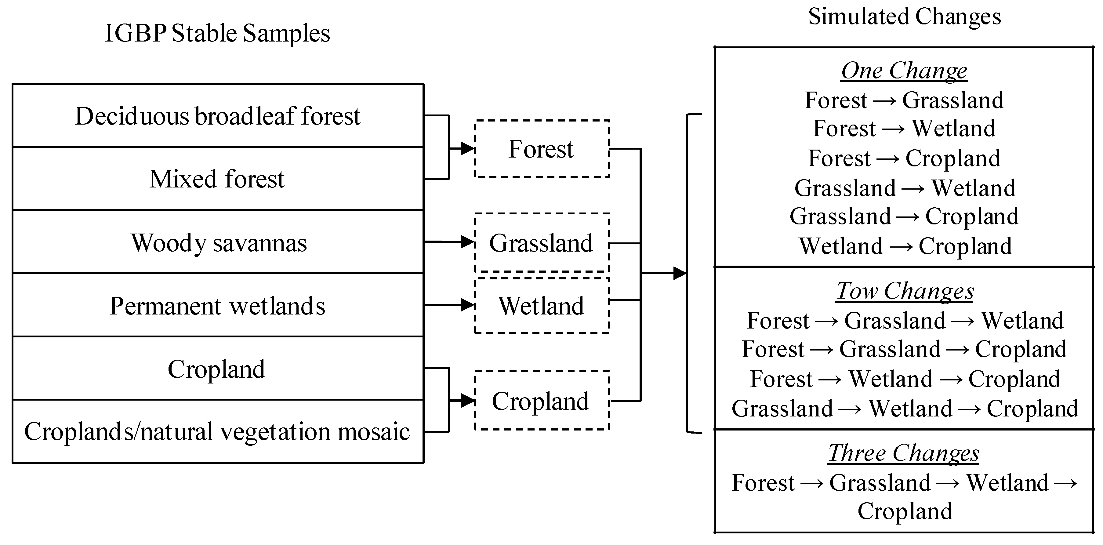
where $t^{\ast }\in \left\{1,2,\mathrm{...},n\right\}$ is the index of the change date. The index $t^{\ast }$ can be simulated by drawing a random number from $\left\{1,2,\mathrm{...},n\right\}$. In addition, the simulated land-cover changes were assumed to obey the rules of a logical transition as defined in Cai et al. [31]. For instance, the simulated time series represent land-cover changes such as forest disturbance (e.g., forest → grassland) or human activities (e.g., grassland → cropland). We have simulated six types of land-cover changes containing one change, four types containing two changes, and one type containing three changes within the same time period of the real NDVI time series. Totally, 1200 time series were simulated for each change intensity level. The stable time series used to simulate changes were randomly selected in each simulation process from the pool of time series of corresponding land-cover classes out of the four grouped classes (Figure 4).

Figure 4. IGBP (International Geosphere–Biosphere Program) stable samples (left); grouped land-cover types (middle) and simulated changes (right).

Figure 4. IGBP (International Geosphere–Biosphere Program) stable samples (left); grouped land-cover types (middle) and simulated changes (right).

The stable IGBP time series were stratified for the six land-cover classes and randomly partitioned into two halves, one for algorithm training and the other for accuracy assessment. Similarly, the simulated time series were randomly partitioned into two halves with stratification for the three change intensities and corresponding change types.

4.1.2. Independent Random Samples

A sub-area encompassing the southern part of Vinton County in southeast Ohio (Figure 1) was selected to validate the performance of the proposed algorithm. According to previous studies [7,32], the land-cover change in this area is highly dynamic as a result of human activities such as logging and reforestation, industrial mining and abandonment, and agricultural use and abandonment. The sub-area contains 60 × 80 columns/rows on a 250-m MODIS image, from which 244 pixels were randomly selected. Major land-cover changes contained in these time series include transitions from forest to bare soil/mining field, forest to cropland, forest to bare soil/mining field and then to grassland, bare soil to grassland, and shrubs to bare soil/mining field. At each of the 244 pixels, the change date(s) of the time series were manually identified to serve as “ground truth” by visual inspection. A series of 94 Landsat images were downloaded from the USGS Landsat archive for the period from 2000 to 2011, including Landsat 5 TM scenes from 2000 to 2011 and Landsat 7 ETM+ scenes from 1999 to 2003. Only images with clear skies over the sub-area were selected. When identifying change dates from the Landsat time series, we tried to convert the time index between Landsat and MODIS as accurately as possible. Nevertheless, it is challenge to obtain the actual “truth”, and the Landsat images do not correspond perfectly to MODIS images in many cases because quite a few of the Landsat images were unavailable due to cloud contamination and/or satellite malfunction. In addition, the exact change date may be confused given that the MODIS 16-day composite data could miss land-cover changes if the changes occurred within the 16-day composite period [17].

4.2. Comparison with BFAST

The proposed method (sub-annual change detection (SCD)) was compared with BFAST developed in Verbesselt et al. [15]. The R package for BFAST version 1.5.7 (published on 28 August 2014) [15,33] was used in R version 3.0.3 (×64) to detect change dates in a time series for comparison. We set the h parameter in BFAST function as 0.08185, which represents the minimal number of observations in each segment (23) divided by the total length of the time series (281). For comparison, we used all trend and seasonal breakpoints detected by BFAST to calculate the accuracy indices.

4.3. Sensitivity Analysis

To analyze the influence of noise and change intensity, we utilized asymmetric Gaussian function to simulate a set of time series representing stable and changes [34,35]. TIMESAT [34,35] was used to analyze the phenological characteristics for each class and nine seasonality parameters were estimated based on the time series in each class. With the estimated seasonality parameters, we simulated time series representing six land-cover classes. Furthermore, we generated land-cover changes with various types and change intensity levels. For each time series generated with asymmetric Gaussian function, we added white noise generated with a normal distribution of zero mean and a series of variance varying from 0.005 to 0.07 with an increment step of 0.005, in order to simulate the noise in NDVI observations. In addition, we added cloud contamination by randomly replace white noise with −0.1 NDVI. Totally, we simulated 600 stable time series with 100 for each of the six land-cover classes. The performance was evaluated by the ratio of false changes. Meanwhile, we simulated 1800 changed time series with 600 for each of the three change intensity levels. The RMSE of change date, RMSE of number of changes, and omission errors were calculated to analyze the sensitivity to noise at different change intensity levels.

The pre-processing step of SCD offers a smoothed time series by identifying cloud conditions and removing white noises with wavelet decomposition. To test the effect of the smoothing techniques used in SCD, we selected a range of decomposition levels, which were used to reconstruct time series from wavelet decomposition, and tested on the 244 independent time series. The decomposition levels range from 0 (no wavelet decomposition applied) to 20, where a greater decomposition level offers smoother time series.

5. Results and Discussion

5.1. IGBP Stable Time Series

Table 2 shows results of applying SCD and BFAST to the IGBP stable time series (i.e., no land-cover change over time) for each land-cover type. The values of the two parameters in SCD were 0.01 for the significance level (α) and 2 for the scale factor (β) based on training with one-fifth of the stable time series. False changes using SCD are very few (zero or one) for each land-cover type given the size of test samples. In contrast, the BFAST method detected more false changes. This indicates that the SCD does not tend to flag false land-cover change.

Table 2. Summary of the results for the stable samples.

IGBP Land-Cover Class	Sample Size		False Change (pixel)
	Train	Test	SCD	BFAST
Deciduous broadleaf forest	30	29	2	22
Mixed forest	39	39	1	26
Woody savannas	11	10	0	1
Permanent wetlands	15	15	0	7
Croplands	103	103	1	48
Croplands/natural vegetation mosaic	4	4	0	0
All	202	200	4	104
Overall accuracy			98%	48%

Notes: train = training samples; test = testing samples; SCD = the proposed sub-annual change detection method; Overall accuracy is calculated as the ration of the overall false changes to the total number of tested stable time series.

Table 2. Summary of the results for the stable samples.

IGBP Land-Cover Class	Sample Size		False Change (pixel)
	Train	Test	SCD	BFAST
Deciduous broadleaf forest	30	29	2	22
Mixed forest	39	39	1	26
Woody savannas	11	10	0	1
Permanent wetlands	15	15	0	7
Croplands	103	103	1	48
Croplands/natural vegetation mosaic	4	4	0	0
All	202	200	4	104
Overall accuracy			98%	48%

Notes: train = training samples; test = testing samples; SCD = the proposed sub-annual change detection method; Overall accuracy is calculated as the ration of the overall false changes to the total number of tested stable time series.

5.2. IGBP Simulated Time Series

Table 3 shows the results of applying SCD to the simulated time series, which represents 11 land-cover change types. The values of 0.075 for α and 1.0 for β were selected with training process. For the time series with intensity at one change, the RMSE of detected change date ranged from 4.6 to 8.2 steps across the six change types, with an overall of 6.8 steps (equivalent to 156 days). The MSE of detected change date ranged from 0.4 to 3.8 steps with an overall of 1.9 steps, indicating slightly overestimated change dates (later than the actual change dates). The RMSE of the number of changes varied around 2 and MSE varied around 1, which means the number of detected changes was overestimated for all six change types. The overall ratio of omission error is 11.2, or 67 out of 600 time series equivalently. Among the six change types, the change from grassland to wetland is associated with the greatest RMSE of detected change date and the most omission errors. A possible reason is that grassland and wetland likely have similar phenological characteristics and similar NDVI values in our dataset (refer to supplementary file). In addition, the time series of grassland and wetland were more sensitive to noise than the other classes (refer to Section 5.3). The change from forest to cropland had the second largest omission errors, which is possibly due to the greater inter-annual variation in the time series for forest or cropland, which can be confused with land-cover change occasionally.

For the time series with intensity at two changes, the RMSE of detected change date ranged from 7 to 9 steps across the four change types. The overall RMSE of detected change date is about 1 step greater than the overall RMSE for the time series with intensity at one change. The MSE of detected change date ranged from −1.9 to 3.0 steps with an overall of 0.6 steps, indicating slightly overestimation about the actual change date. The RMSE from 1.5 to 1.8 with an overall of 1.6, and MSE of the number of change ranged from 0.4 to 0.9, which are more accurate when compared with the results for the intensity at one change. In addition, the overall ratio of omission error is also smaller than that for the time series with intensity at one change. The results are interesting because the four change types simulated for the intensity at two changes are actually four different combinations of the six change types simulated for the intensity at one change; and the accuracy values are in certain degree mimic the average of the accuracy values for the associated change types.

One change type was simulated for time series with intensity at three changes. The values of the five indices are close to the overall values of the indices for the time series with intensity at two changes.

Table 3. Summary of the results for the simulated time series with changes.

Number of Changes	Land-Cover Transitions (Sample Size)	Time Steps		Number		Omission Error (%)
		RMSE	MSE	RMSE	MSE
1	forest → grassland (100)	6.6	2.8	2.3	1.5	1.2
	forest → wetland (100)	7.7	3.8	2.2	1.3	1.8
	forest → cropland (100)	7.7	1.8	1.7	0.7	3.5
	grassland → wetland (100)	8.2	0.5	2.1	0.8	4.0
	grassland → cropland (100)	6.7	0.4	1.3	0.9	0.2
	wetland → cropland (100)	4.6	1.8	1.9	1.4	0.5
	Overall (600)	6.8	1.9	2.0	1.1	11.2
2	forest → grassland → wetland (150)	9.0	-1.9	1.7	0.4	3.7
	forest → grassland → cropland (150)	7.3	0.5	1.6	0.7	1.0
	forest →wetland →cropland (150)	7.5	0.1	1.8	0.9	1.3
	grassland →wetland →cropland (150)	8.1	3.0	1.5	0.7	0.3
	Overall (600)	8.0	0.6	1.6	0.7	6.3
3	forest → grassland → wetland → cropland (600)	7.2	0.3	1.9	0.5	7.3

Note: Time steps stands for the time of detected change in the unit of step, i.e., 16 days; number stands for the number of changes.

Table 3. Summary of the results for the simulated time series with changes.

Number of Changes	Land-Cover Transitions (Sample Size)	Time Steps		Number		Omission Error (%)
		RMSE	MSE	RMSE	MSE
1	forest → grassland (100)	6.6	2.8	2.3	1.5	1.2
	forest → wetland (100)	7.7	3.8	2.2	1.3	1.8
	forest → cropland (100)	7.7	1.8	1.7	0.7	3.5
	grassland → wetland (100)	8.2	0.5	2.1	0.8	4.0
	grassland → cropland (100)	6.7	0.4	1.3	0.9	0.2
	wetland → cropland (100)	4.6	1.8	1.9	1.4	0.5
	Overall (600)	6.8	1.9	2.0	1.1	11.2
2	forest → grassland → wetland (150)	9.0	-1.9	1.7	0.4	3.7
	forest → grassland → cropland (150)	7.3	0.5	1.6	0.7	1.0
	forest →wetland →cropland (150)	7.5	0.1	1.8	0.9	1.3
	grassland →wetland →cropland (150)	8.1	3.0	1.5	0.7	0.3
	Overall (600)	8.0	0.6	1.6	0.7	6.3
3	forest → grassland → wetland → cropland (600)	7.2	0.3	1.9	0.5	7.3

Note: Time steps stands for the time of detected change in the unit of step, i.e., 16 days; number stands for the number of changes.

5.3. Results of Sensitivity Analysis

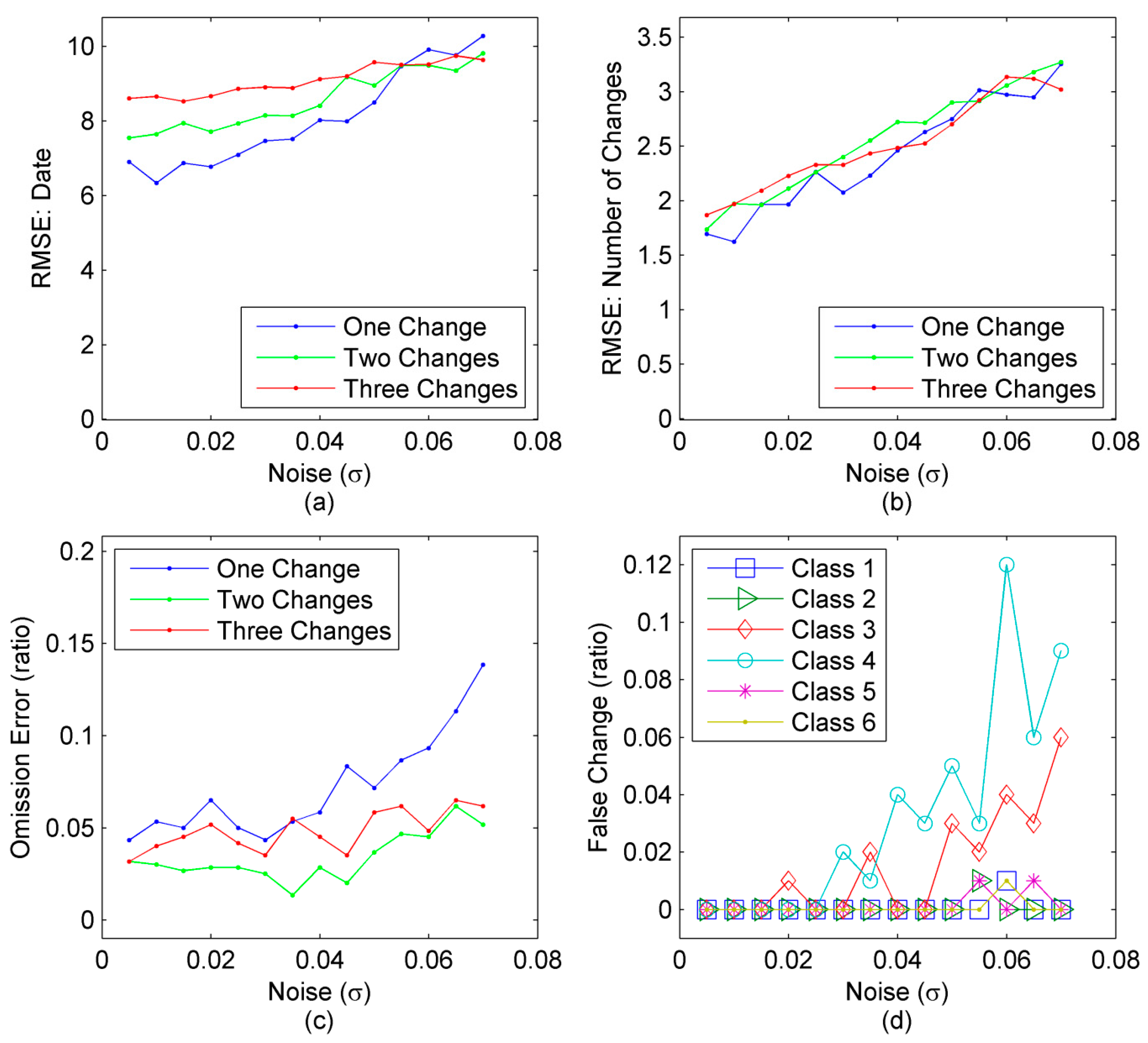
Figure 5a–c illustrates the effect of noise on SCD when it was applied to the time series with simulated land-cover changes. When noise level increased, accuracy decreased. For the change intensity, the RMSE of change date (Figure 5a) became greater from one change to three changes at noise level (represented by sigma σ) smaller than 0.05, but varied little across the three change intensities at noise level greater than 0.05. On the other hand, the omission errors (Figure 5c) are greater and increased more rapidly with noise for time series with intensity at one change than two or three changes. Meanwhile, the RMSE of the number of change does not show much difference among the three change intensities even when noise level increased; the variability of the RMSE for the intensity at one change is slightly larger than the other two change intensities (Figure 5b). It is noted that the simulated time series with intensity at one change consist of six change types characterized with large variability among time series and thus were more sensitive to noise, compared to the simulated time series with intensity at three changes which only represent one change type.

Figure 5d shows the influence of noise on the performance of SCD when it was applied to the stable time series, assessed by the ratio of false change to the total number of stable time series for each land-cover class. For all six classes, the ratio of false change increased slightly, e.g., from 0 to 0.01–0.12, when the noise level increased from 0.01 to 0.07. The ratio of false change in the class of broadleaf deciduous forest, cropland, mixed forest and cropland mosaic (class 1, 2, 5 and 6) shows very small variation with noise. In contrast, the ratios for the class of woody savanna and permanent wetland (class 3 and 4) have great variations when the noise level is greater than 0.02.

Figure 5. The influence of noise and change intensity on the RMSE of change time (a); RMSE of number of changes (b); and omission errors (c) of simulated time series, and the influence of noise on stable time series represented by the ratio of false change calculated for Classes 1–6 (d). In each plot, the X-axis represents the standard deviation (σ) of white noise added to the time series.

Figure 5. The influence of noise and change intensity on the RMSE of change time (a); RMSE of number of changes (b); and omission errors (c) of simulated time series, and the influence of noise on stable time series represented by the ratio of false change calculated for Classes 1–6 (d). In each plot, the X-axis represents the standard deviation (σ) of white noise added to the time series.

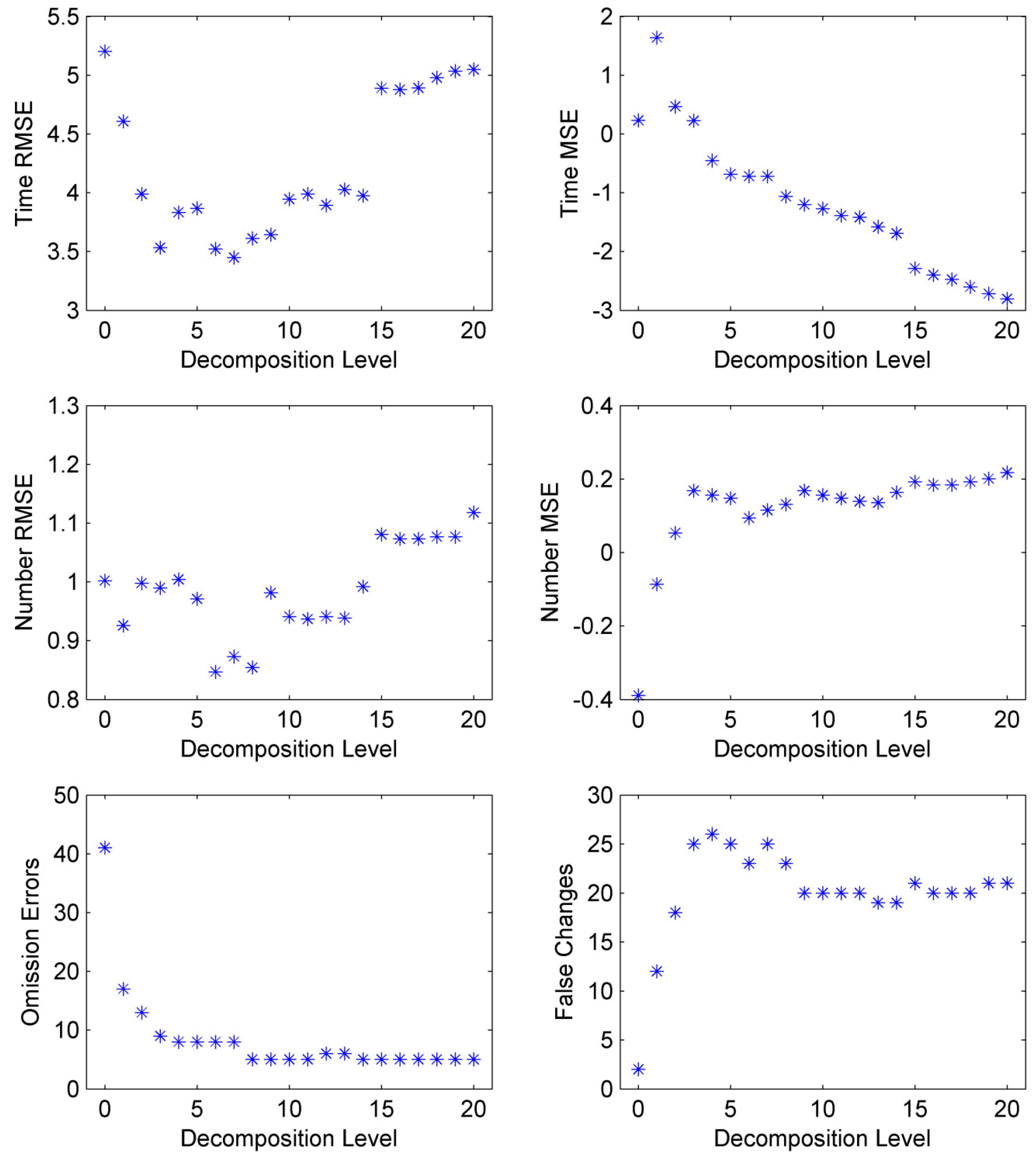
Figure 6 shows the smoothing effect on six accuracy indices when SCD is applied to the 244 independent time series in the sub-area. When the smoothing level increased from 0 to 5, the RMSE of change date, the RMSE of the number of changes, and omission errors decreased rapidly, indicating greater accuracy of the detected change date and number of changes; meanwhile, the MSE of the number of changes increased from negative to positive, or from underestimation to overestimation, and the number of false changes increased. When the smoothing level increased from 6 to 20, the RMSE of change date rebounded to the values without smoothing, the RMSE of the number of changes increased to greater values, and the MSE of change date became more negative, while the other indices had little variation. Briefly, the smoothing process at low or intermediate level (i.e., level ≤ 5) improved the accuracy of the detected changes with sacrifice of false changes, but too much smoothing reduced the accuracy of the detected change date and did not improve the accuracy of other indices.

Figure 6. Plots of smoothing effect on the accuracy indices, which were calculated based on independent random samples. The accuracy indices as shown on the Y-axis are the RMSE and MSE of time step (Time RMSE and Time MSE), the RMSE and MSE of the number of changes (Number RMSE and Number MSE), the omission errors of changes in percentage (Omission Errors) and the false changes in stable time series in percentage (False Changes). The X-axis is the wavelet decomposition level, which is used to reconstruct time series from wavelet decomposition.

Figure 6. Plots of smoothing effect on the accuracy indices, which were calculated based on independent random samples. The accuracy indices as shown on the Y-axis are the RMSE and MSE of time step (Time RMSE and Time MSE), the RMSE and MSE of the number of changes (Number RMSE and Number MSE), the omission errors of changes in percentage (Omission Errors) and the false changes in stable time series in percentage (False Changes). The X-axis is the wavelet decomposition level, which is used to reconstruct time series from wavelet decomposition.

5.4. Independent Random Samples

Results for the random samples extracted from the sub-area are shown in Table 4. The values of the two parameters used in the simulated time series (refer to Section 4.3) were utilized to generate results for the random samples. Within the 244 samples, 77 time series represent changed land cover and 167 represent stable land cover. The SCD had greater omission errors than BFAST for changed land cover, but fewer false changes for stable land cover. Such results indicate the SCD is more conservative compared to BFAST and tends to detect real change instead of false change with some degree of omissions. For the changed time series, SCD has a MSE of 0.06 for the number of detected changes and BFAST a MSE of 0.22, which is consistent with the characteristics indicated by omission errors. SCD generated a RMSE of 0.84 for the number of detected changes, which is very close to the RMSE for BFAST.

Table 4. Summary of the results for the random samples in the sub-area.

Method	Stable (167)	Changed (77)					Computational Time (Second)
	False Change (pixel)	Omission Error (pixel)	Time Step		Number
			RMSE	MSE	RMSE	MSE
SCD	21	15	4.05	−0.26	0.93	0.10	16
BFAST	49	6	6.02	0.25	0.86	0.20	635

Note: in the first row, stable represents stable land-cover samples, and changed represents changed land-cover samples, and the number in the parenthesis is the number of samples; time step stands for the time of detected changes in the unit of step (16 days), and number stands for the number of detected changes.

Table 4. Summary of the results for the random samples in the sub-area.

Method	Stable (167)	Changed (77)					Computational Time (Second)
	False Change (pixel)	Omission Error (pixel)	Time Step		Number
			RMSE	MSE	RMSE	MSE
SCD	21	15	4.05	−0.26	0.93	0.10	16
BFAST	49	6	6.02	0.25	0.86	0.20	635

Note: in the first row, stable represents stable land-cover samples, and changed represents changed land-cover samples, and the number in the parenthesis is the number of samples; time step stands for the time of detected changes in the unit of step (16 days), and number stands for the number of detected changes.

The SCD was more accurate in determining the time of detected change compared to BFAST. SCD generated a RMSE of 4 steps, or the equivalent of about two months from the actual change time, whereas the BFAST had a RMSE of six steps, which is equivalent to more than three months. According to the MSE, the time of detected change estimated by both methods was later than the actual time in most cases, though SCD generated smaller bias than BFAST.

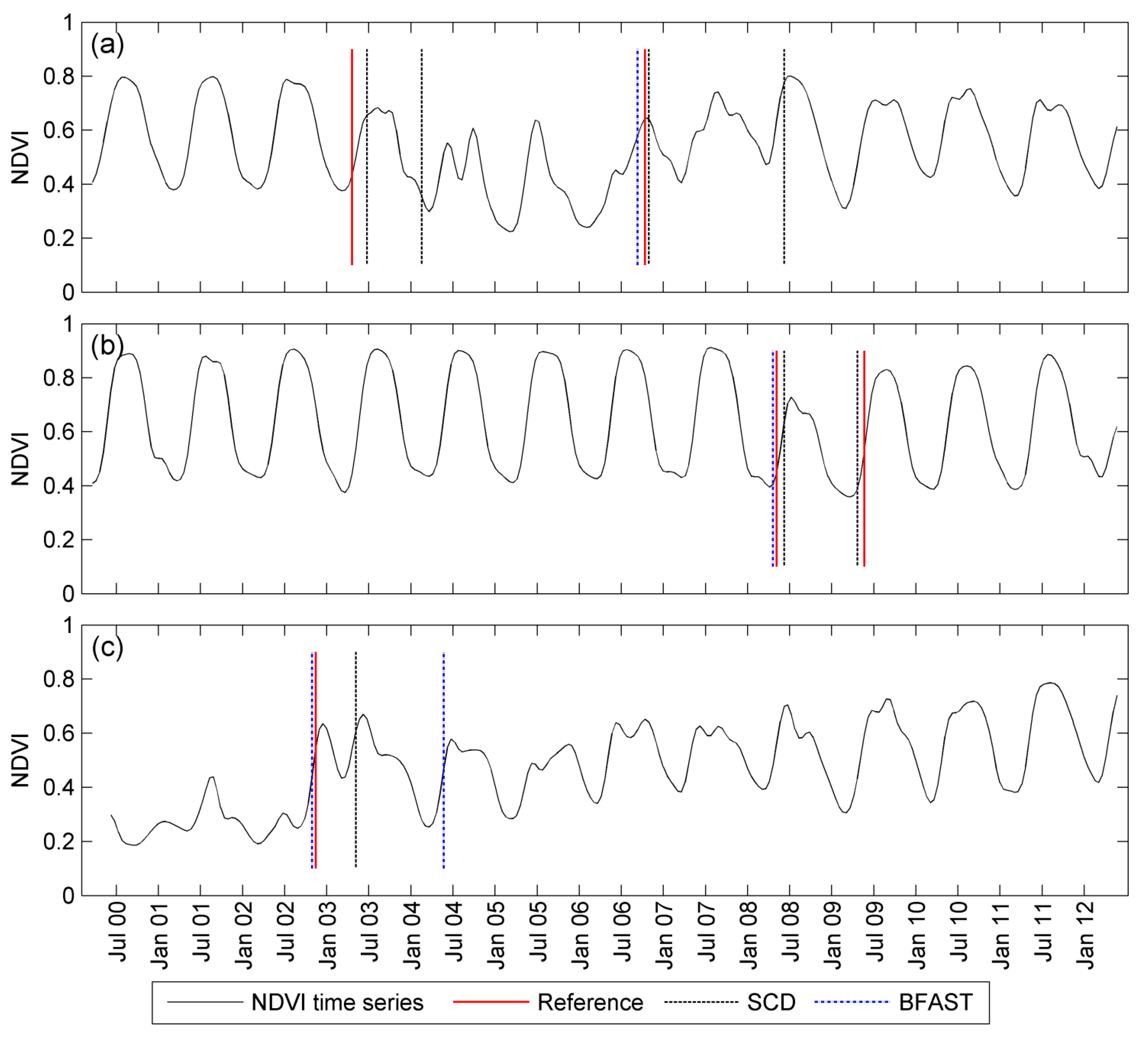
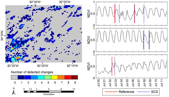
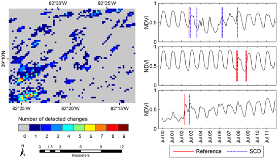
Figure 7 shows the examples of changes detected in the time series for three pixels. The time series in Figure 7a recorded the changes from forest to bare soil earlier in the period (i.e., the forest had been cleared for industrial mining) and a return of grassland years later. According to visual inspection of the Landsat time series data, the two changes occurred in April 2003 and October 2006. SCD detected four changes, two of which matched the time of the actual changes identified from the time series of Landsat images. The other two also corresponded to observable shifts in NDVI values, though they may not have been associated with land-cover changes, or at least the changes were not recorded by the Landsat images. In contrast, BFAST only detected one change, the time of which was close to the second observed change in October 2006. Figure 7b shows a time series with similar land-cover trajectories, from forest to bare soil and then to grassland, as the time series in Figure 7a. SCD detected both change dates and they are close to the reference dates, which is more accurate than the result of BFAST for this time series. The time series shown in Figure 7c recorded a change from bare soil to grassland, where the change date detected by SCD is less accurate than the first change date detected by BFAST. The examples illustrate how SCD can be used to detect land-cover changes in a time series.

The computation time required for the two methods is also reported in Table 4. The proposed SCD method cost much less time for processing 244 time series compared to the BFAST algorithm. Computation time may be a critical issue when large number of time series need to be analyzed, such as with global datasets.

Figure 7. Examples of detected changes for three 16-day NDVI time series (smoothed) extracted from three MODIS pixels at 250 m resolution in southeast Ohio (tile h11v05). The corresponding land-cover changes are forest → bare soil → grassland (a,b) and bare soil → grassland (c).

Figure 7. Examples of detected changes for three 16-day NDVI time series (smoothed) extracted from three MODIS pixels at 250 m resolution in southeast Ohio (tile h11v05). The corresponding land-cover changes are forest → bare soil → grassland (a,b) and bare soil → grassland (c).

5.5. Spatial Patterns in the Sub Area

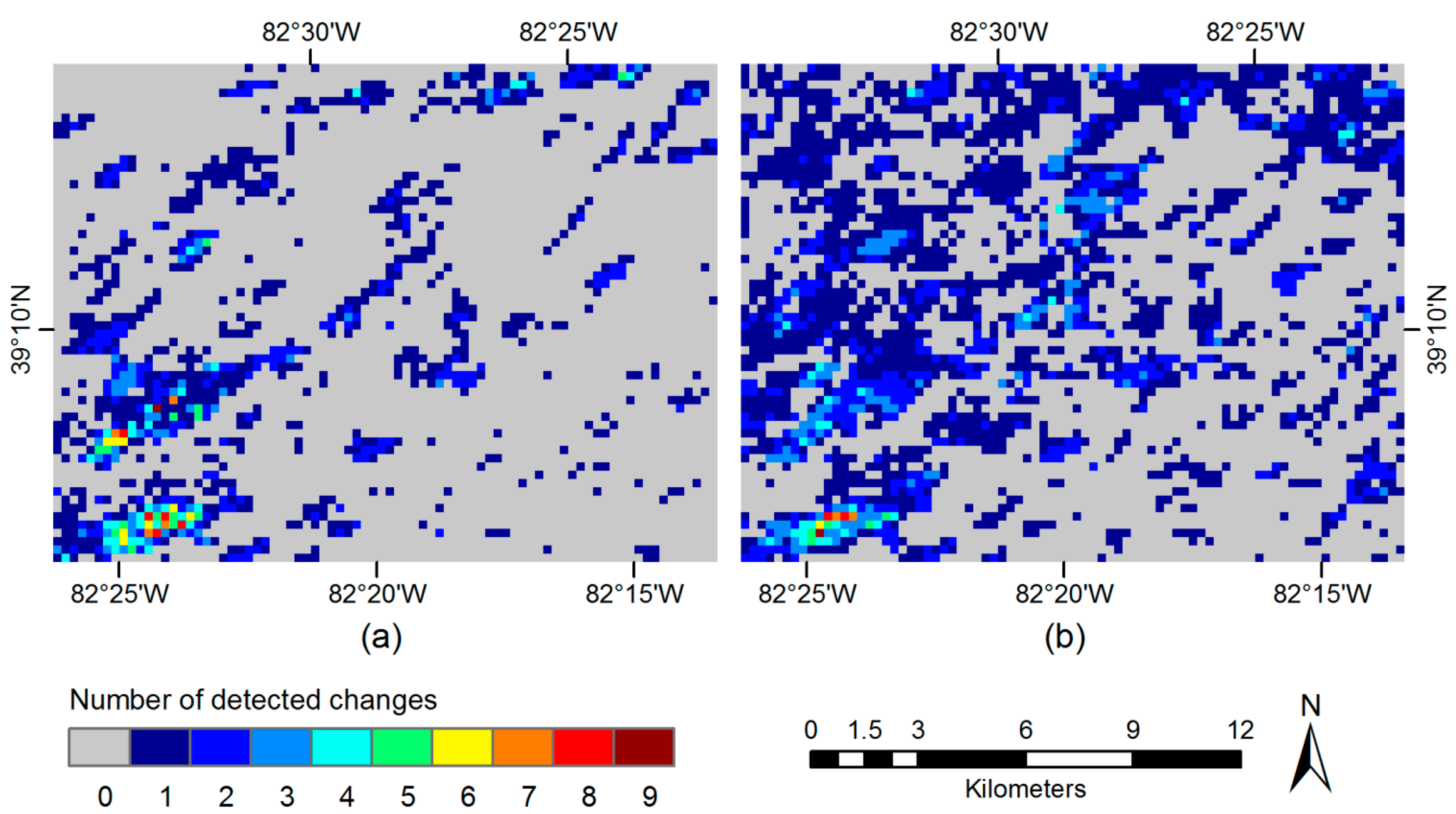
The SCD and BFAST methods were applied to all time series in the sub-area, and maps of the number of detected changes are shown in Figure 8. On the map generated by SCD, the sub-area was dominated with pixels that did not change from 2000 to 2010. Within the changed areas, most pixels have changed once or twice within the 13 years, which likely corresponds to forest clearing for agricultural activities or urban development. In contrast, the map generated by BFAST has more pixels that changed once or twice than pixels with stable land cover. The southeast parts of both maps showed more changes (i.e., about 3–9 times per pixel), which were likely associated with forest clearing for industrial mining (bare soil) in the early 2000s, abandonment later and return of vegetation (i.e., grassland, shrubland, etc.) in the late 2000s or early 2010s. With the moderate (250 m) spatial resolution of MODIS NDVI data, it could be clearly seen that neighboring pixels exhibited spatial continuity in change frequencies and possibly similar change dates as well.

Figure 8. Maps of detected changes from 2000 to 2012 generated by the proposed method (a) and BFAST (b). The extent of the map corresponds to the sub-area as shown in Figure 1. The color of a pixel is coded by its value according to the color bar on the bottom left. The pixel values equal the number of detected changes during the entire time period. Zero means no change.

Figure 8. Maps of detected changes from 2000 to 2012 generated by the proposed method (a) and BFAST (b). The extent of the map corresponds to the sub-area as shown in Figure 1. The color of a pixel is coded by its value according to the color bar on the bottom left. The pixel values equal the number of detected changes during the entire time period. Zero means no change.

6. Strengths and Limitations of SCD

The increasing availability of dense time series satellite images makes it possible to detect land-cover changes at improved temporal resolutions. Most previous change detection methods are based on bi-temporal or multi-year image data, which can identify changes only at the resolution of years. The proposed SCD method is designed for dense time series and it can detect land-cover changes at the resolution of days. Traditional change detection methods use annual images to avoid seasonal variations, which cannot be directly applied to dense time series. In contrast, SCD accounts for seasonal variations in dense time series and differentiate land-cover change from phenological change in a year. In addition, like BFAST, SCD can detect a variety of land-cover changes rather than focusing on forest changes as in previous studies using dense time series of images (e.g., [6,9]).

The SCD method detects change dates by analyzing time series differences on yearly and 16-day scales coherently. It detects the years that include land-cover changes before detecting change dates by applying a two-sample KS test, which can reduce error in the time of detected change to less than a year. In addition, the SCD method does not require much prior information. The method can be applied to observations spanning any two consecutive years to detect change dates in the second year, regardless of the starting time point; observation records of full year in each one is not required though observations spanning over half a year is necessary to guarantee the accuracy. This is advantageous for detecting change dates in time series with continuously updated observations. In addition, the parameter settings do not need to be calibrated for different land-cover classes or different time periods. Lastly, SCD is computationally efficient by using a hierarchical approach and thus can be easily applied to large data sets.

The two parameters are critical for detecting change dates accurately and can be determined through a training process. The significance level for a KS test determines whether or not changes occurred within a year. The result of the KS test directly affects the accuracy of the number of detected changes and indirectly influences the accuracy of the time of detected change (in which year a change occurred). When a time series has great intra-annual variation, such as crops with rotation or double cropping, accurately detecting land-cover change will be challenging. Changes are sensitive to the significance level in such cases. The other parameter is the scale factor used to determine the change dates in a year. Using the maximum of the absolute difference between two years’ records, it defines the threshold at which a land-cover change can be detected. The value of the scale factor is the same for all time series as selected by the training data, but the maximum is unique for different years or time series. Therefore, the threshold is adaptive to the characteristics of a particular time series in a certain year. The idea of studying the difference between two time series is borrowed from the bands-difference method for traditional change detection. In the SCD, the threshold is used to determine change points in the time domain. The training samples used to determine the parameters in this study consisted of only simulated time series. Real time series with reference information may better serve for training but are very limited in terms of sample size. Future effort will be focused on obtaining more samples of real time series that have more complex changing patterns (i.e., more than three changes) to improve the training process. The SCD also needs further validation with more study sites.

A limitation of the SCD algorithm is that the minimum time period between two neighboring change dates is one year, because we always compare the records on the same dates in two years. Specifically, when a change date is detected in one year, only the records on the dates later than the change date in that year and the following year will be compared, which generates at least a year difference between two change dates. This limit may affect the detection accuracy when actual land-cover changes are more frequent than a year, which, however, is a rare case in the real world. In addition, observations recorded in the same seasons of two years are necessary for SCD to detect the change date in the second year, because SCD compares the seasonal pattern recorded in the two years and searches the change point at which the seasonal pattern started to represent a different land cover. Such requirement on time series can reasonably determine a land-cover change rather than inter-annual variation. Although it is rarely observed, persistent cloud cover would affect the accuracy of the result. In fact, observation records spanning more than six months (i.e., satisfying Nyquist frequency of a year) are necessary to generate meaningful results in the interpolation process.

Year-to-year seasonal changes (or inter-annual variation) commonly exist in NDVI time series, such as changes in lengths of seasons from one year to another, possibly due to drought, floods, different snow onset time, or other harsh conditions. Such inter-annual variations are considered as noise in the sub-annual change detection process and should not be confused with land-cover change. For instance, the results on the stable time series in Table 2 showed small errors in false changes detected by SCD, as well as the fewer false changes in Table 4 compared to BFAST. Because SCD is designed to differentiate abrupt land-cover change from inter-annual variation, it is less influenced by inter-annual variations within stable time series. Nevertheless, certain inter-annual variation could bring about challenge in sub-annual change detection and affect the detection accuracy when the variation is not observed in reference data or determined as abrupt land-cover changes (e.g., due to slow process of modification).

7. Conclusions

A sub-annual change detection (SCD) method was proposed in this study in order to detect dates of abrupt land-cover change on sub-annual scale (i.e., 16-day step) from very dense time series of satellite images. The proposed method divides time series into annual segments and statistically detects changes in each segment. It estimates change dates by analyzing differences between two consecutive annual segments at yearly and time-point scales coherently. Additionally, it does not require prior information about land-cover types or change trajectory, which is often necessary for existing methods. Detected change dates can be used to determine appropriate segments of a time series for land-cover trajectory mapping and also facilitate studies of land surface processes, which require specific information about land surface changes.

The simulated time series with various land-cover classes and change types confirm that the proposed method can be applied to a range of time series representing a wide variety of land surface changes and disturbances. The method was applied to MODIS 16-day NDVI time series (2000–2010) for a study site in southeastern Ohio, USA. The results show that the proposed method is capable of detecting change dates with various types of change trajectories representing the transitions among different vegetated land-cover classes. The results were also compared with the BFAST [15] method, which offers estimation of breakpoints in a time series for trend and seasonal changes about vegetated land covers. Although the proposed method does not differentiate trend and seasonal changes, the comparison suggests that both methods can detect change dates from NDVI time series with similar accuracy (e.g., with RMSE of 4.05 and 6.02 steps for the detected change date using the proposed method and BFAST, respectively) and the proposed method is more computationally efficient (e.g., spent 16 seconds, vs. 635 seconds for BFAST, for 244 samples). The high efficiency can improve the processing of large data sets on both regional and global scales.

The change detection analysis at sub-annual basis ought not to be limited to MODIS data only but other data source providing frequent and regular observations with higher spatial resolution. For instance, the coarse spatial resolution of MODIS data may be inadequate to detect land-cover changes, which occurred in fine spatial resolution (i.e., sub-pixel level). Future research is expected to test the method in other areas and with data sources of finer spatial resolution. It is also important to explore application with irregular observations with the development of blending techniques between high spatial resolution sensor (e.g., Landsat TM) and high temporal resolution sensor (e.g., MODIS), as well as advancement of technology in satellite constellation operation (e.g., RapidEye).

References

- Meyer, W.B.; Turner, I.B.L. Changes in Land Use and Land Cover: A Global Perspective; Cambridge University Press: Cambridge, UK, 1994. [Google Scholar]
- Vitousek, P.M.; Mooney, H.A.; Lubchenco, J.; Melillo, J.M. Human domination of earth’s ecosystems. Science 1997, 277, 494–499. [Google Scholar] [CrossRef]
- Coppin, P.; Jonckheere, I.; Nackaerts, K.; Muys, B.; Lambin, E. Digital change detection methods in ecosystem monitoring: A review. Int. J. Remote Sens. 2004, 25, 1565–1596. [Google Scholar] [CrossRef]
- Lu, D.; Mausel, P.; Brondizio, E.; Moran, E. Change detection techniques. Int. J. Remote Sens. 2004, 25, 2365–2407. [Google Scholar] [CrossRef]
- Kennedy, R.E.; Cohen, W.B.; Schroeder, T.A. Trajectory-based change detection for automated characterization of forest disturbance dynamics. Remote Sens. Environ. 2007, 110, 370–386. [Google Scholar] [CrossRef]
- Huang, C.; Goward, S.N.; Masek, J.G.; Thomas, N.; Zhu, Z.; Vogelmann, J.E. An automated approach for reconstructing recent forest disturbance history using dense landsat time series stacks. Remote Sens. Environ. 2010, 114, 183–198. [Google Scholar] [CrossRef]
- Liu, D.; Cai, S. A spatial-temporal modeling approach to reconstructing land-cover change trajectories from multi-temporal satellite imagery. Ann. Assoc. Am. Geogr. 2012, 102, 1329–1347. [Google Scholar] [CrossRef]
- Kaufmann, R.K.; Seto, K.C. Change detection, accuracy, and bias in a sequential analysis of landsat imagery in the pearl river delta, china: Econometric techniques. Agric. Ecosyst. Environ. 2001, 85, 95–105. [Google Scholar] [CrossRef]
- Kennedy, R.E.; Yang, Z.; Cohen, W.B. Detecting trends in forest disturbance and recovery using yearly landsat time series: 1. Landtrendr—Temporal segmentation algorithms. Remote Sens. Environ. 2010, 114, 2897–2910. [Google Scholar] [CrossRef]
- Basseville, M.; Nikiforov, V. Detection of Abrupt Changes: Theory and Application; Prentice-Hall: Englewood Cliffs, NJ, USA, 1993. [Google Scholar]
- Keogh, E.; Chu, S.; Hart, D.; Pazzani, M. Segmenting time series: A survey and novel approach. In Data Mining in Time Series Databases; Last, M., Kandel, A., Bunke, H., Eds.; World Scientific Publishing Company: Singapore, 2004; Volume 57, pp. 1–22. [Google Scholar]
- Olsen, L.R.; Chaudhuri, P.; Godtliebsen, F. Multiscale spectral analysis for detecting short and long range change points in time series. Comput. Stat. Data Anal. 2008, 52, 3310–3330. [Google Scholar] [CrossRef]
- Sharifzadeh, M.; Azmoodeh, F.; Shahabi, C. Change detection in time series data using wavelet footprints. Lect. Notes Comput. Sci. 2005, 3633, 127–144. [Google Scholar]
- Goodwin, N.R.; Collett, L.J. Development of an automated method for mapping fire history captured in landsat tm and etm plus time series across queensland, australia. Remote Sens. Environ. 2014, 148, 206–221. [Google Scholar] [CrossRef]
- Verbesselt, J.; Hyndman, R.; Newnham, G.; Culvenor, D. Detecting trend and seasonal changes in satellite image time series. Remote Sens. Environ. 2010, 114, 106–115. [Google Scholar] [CrossRef]
- Jamali, S.; Jonsson, P.; Eklundh, L.; Ardo, J.; Seaquist, J. Detecting changes in vegetation trends using time series segmentation. Remote Sens. Environ. 2015, 156, 182–195. [Google Scholar] [CrossRef]
- MODIS. Modis Vegetation Index (mod 13): Algorithm Theoretical Basis Document (Version 3). Available online: http://modis.Gsfc.Nasa.Gov/data/atbd/atbd_mod13.Pdf (accessed on 1 June 2012).
- Lunetta, R.S.; Knight, J.F.; Ediriwickrema, J.; Lyon, J.G.; Worthy, L.D. Land-cover change detection using multi-temporal modis ndvi data. Remote Sens. Environ. 2006, 105, 142–154. [Google Scholar] [CrossRef]
- Short, N. The Landsat Tutorial Workbook: Basics of Satellite Remote Sensing; publication 1078; NASA: Washington, DC, USA, 1992. [Google Scholar]
- Lambin, E.F.; Strahler, A.H. Change-vector analysis in multitemporal space—A tool to detect and categorize land-cover change processes using high temporal-resolution satellite data. Remote Sens. Environ. 1994, 48, 231–244. [Google Scholar] [CrossRef]
- Viovy, N.; Arino, O.; Belward, A.S. The best index slope extraction (bise): A method for reducing noise in ndvi time-series. Int. J. Remote Sens. 1992, 13, 1585–1590. [Google Scholar] [CrossRef]
- Bruce, L.M.; Mathur, A.; Byrd, J.A. Denoising and wavelet-based feature extraction of MODIS multi-temporal vegetation signatures. GISci. Remote Sens. 2006, 43, 67–77. [Google Scholar] [CrossRef]
- Burrus, C.S.; Guo, R.A.G.H. Introduction to Wavelets and Wavelet Transforms: A Primer; Prentice Hall: Upper Saddle River, NJ, USA, 1998. [Google Scholar]
- Ben Aissa, M.S.; Boutahar, M.; Jouini, J. Bai and perron’s and spectral density methods for structural change detection in the us inflation process. Appl. Econ. Lett. 2004, 11, 109–115. [Google Scholar] [CrossRef]
- Wang, W.; Chen, X.; Shi, P.; van Gelder, P. Detecting changes in extreme precipitation and extreme streamflow in the dongjiang river basin in southern china. Hydrol. Earth Syst. Sci. 2008, 12, 207–221. [Google Scholar] [CrossRef]
- Deshayes, J.; Picard, D. Off-line statistical-analysis of change-point models using non parametric and likelihood methods. Lect. Notes Control Inf. Sci. 1986, 77, 103–168. [Google Scholar]
- Massey, F.J., Jr. The kolmogorov-smirnov test for goodness of fit. J. Am. Stat. Assoc. 1951, 46, 68–78. [Google Scholar] [CrossRef]
- Loveland, T.R.; Belward, A.S. The igbp-dis global 1 km land cover data set, discover: First results. Int. J. Remote Sens. 1997, 18, 3291–3295. [Google Scholar] [CrossRef]
- Friedl, M.A.; Sulla-Menashe, D.; Tan, B.; Schneider, A.; Ramankutty, N.; Sibley, A.; Huang, X.M. Modis collection 5 global land cover: Algorithm refinements and characterization of new datasets. Remote Sens. Environ. 2010, 114, 168–182. [Google Scholar] [CrossRef]
- Friedl, M.A.; McIver, D.K.; Hodges, J.C.F.; Zhang, X.Y.; Muchoney, D.; Strahler, A.H.; Woodcock, C.E.; Gopal, S.; Schneider, A.; Cooper, A.; et al. Global land cover mapping from modis: Algorithms and early results. Remote Sens. Environ. 2002, 83, 287–302. [Google Scholar] [CrossRef]
- Cai, S.; Liu, D.; Sulla-Menashe, D.; Friedl, M. Enhancing modis land cover product with a spatial-temporal modeling algorithm. Remote Sens. Environ. 2014, 147, 243–255. [Google Scholar] [CrossRef]
- McSweeney, K.; McChesney, R. Outbacks: The popular construction of an emergent landscape. Landsc. Res. 2004, 29, 31–56. [Google Scholar] [CrossRef]
- Verbesselt, J.; Hyndman, R.; Zeileis, A.; Culvenor, D. Phenological change detection while accounting for abrupt and gradual trends in satellite image time series. Remote Sens. Environ. 2010, 114, 2970–2980. [Google Scholar] [CrossRef]
- Jonsson, P.; Eklundh, L. Seasonality extraction by function fitting to time-series of satellite sensor data. IEEE Trans. Geosci. Remote Sens. 2002, 40, 1824–1832. [Google Scholar] [CrossRef]
- Jonsson, P.; Eklundh, L. Timesat—A program for analyzing time-series of satellite sensor data. Comput. Geosci. 2004, 30, 833–845. [Google Scholar] [CrossRef]
© 2015 by the authors; licensee MDPI, Basel, Switzerland. This article is an open access article distributed under the terms and conditions of the Creative Commons Attribution license (http://creativecommons.org/licenses/by/4.0/).