A Robust Fuzzy Neural Network Model for Soil Lead Estimation from Spectral Features

Abstract

Soil lead content is an important parameter in environmental and industrial applications. Chemical analysis, the most commonly method for studying soil samples, are costly, however application of soil spectroscopy presents a more viable alternative. The first step in the method is usually to extract some appropriate spectral features and then regression models are applied to these extracted features. The aim of this paper was to design an accurate and robust regression technique to estimate soil lead contents from laboratory observed spectra. Three appropriate spectral features were selected according to information from other research as well as the spectrum interpretation of field collected soil samples containing lead. These features were then applied to common Multiple Linear Regression (MLR), Partial Least Square Regression (PLSR) and Neural Network (NN) regression models. Results showed that although NN had adequate accuracy, it produced unstable results (i.e., variation of response in different runs). This problem was addressed with application of a Fuzzy Neural Network (FNN) with a least square training strategy. In addition to the stabilized and unique response, the capability of the proposed FNN was proved in terms of regression accuracy where a Ratio of Performance to Deviation (RPD) of 8.76 was achieved for test samples.

1. Introduction

Accurate and reliable estimation of heavy metal contents in soil samples is important for environmental studies. Any increased concentration of such elements like lead (Pb) in soil presents a health threat to most creatures and humans [1,2,3]. Extraction of these elements is also important for several industrial applications such as ammunition, burial vault liners, ceramic glazes, leaded class and crystal and water lines and pipes [4].

Traditionally, Pb contents in soils have been determined in a laboratory where prepared soil samples are subjected to expensive and time consuming analysis [2,5,6]. Regarding access to high resolution and accurate spectral data (which are obtained via field spectrometry or space-born hyper spectral imaging), spectroscopy is an appropriate alternative to the afore-mentioned traditional chemical analysis [7,8,9,10].

Various researches have made determinations of lead using remotely sensed spectral data. Choe et al. (2008) reports the following evaluations from a linear regression model; a relation between spectral parameters of R_610,500 band ratio, occupied area of A₅₀₀ and Pb content. RPD value of 1.39, and these research results confirmed inappropriateness of the linear models for estimating Pb concentration [7].

Wu et al. (2005) introduced an appropriate relationship between VIS-NIR spectral range and the soil Pb concentrations using Partial Least Square Regression (PLSR). An evaluation of R² = 0.81 from the PLSR model showed high level ability of this model for making determinations of Pb concentration. The report demonstrated that the PLSR model is more precise for estimating other elements, mercury and chromium compared to Pb [11].

Ko et al. (2004) attempted to use the PLSR model and principal components to estimate the Pb concentrations in compost. Comparison between models (the Modified Partial Least Square (MPLS), PLSR and Principle Component Regression (PCR)) showed that MPLS had better ability to estimate the Pb concentrations. According to R² < 0.81 for the mentioned models, it was concluded that linear models did not demonstrate enough accuracy to estimate the Pb concentrations in compost [12]. Choe et al. (2009) introduced the range of 400 nm–2400 nm as the most appropriate range for regression modeling of heavy metals. Results showed that the linear model was not appropriate for making estimations for the Pb concentrations [13].

Farifteh et al. (2007) compared linear and non-linear models PLSR and Artificial Neural Network (ANN) respectively, in terms of estimations for salt in soil samples. These models are implemented and compared using different data sets. According to the obtained RPD > 2.1, the ability of both models was confirmed for estimating levels of salt in soil samples [9]. Liu et al. (2011) used neural network models to estimate heavy metals concentrations (e.g., copper and cadmium) in rice using spectral indices and environmental parameters. These tests concluded that appropriate combination of spectral indices did improve results of estimations [14].

The objective of this research was to design an accurate and reliable model to estimate soil Pb content from its reflectance spectra. This was done by selecting three appropriate spectral features, including band ratios of R_610,860, R_1000,1342 and A500. These features were then introduced to previews of common regression models such as MLR, PLSR and NN. Considering the insufficient accuracy of MLR and PLSR as well the instability defect of NN, a robust Fuzzy Neural Network (FNN) model was then proposed and evaluated.

2. A Review on Regression Models: State-of-the-Art

In this section, the applied regression models are reviewed according to two general categories: linear and non-linear models. Multiple Linear Regression (MLR) and Partial Least Square Regression (PLSR) models were selected as the most conventional linear models, and Neural Network (NN) and Fuzzy Neural Network (FNN) are reviewed as the most flexible non-linear methods. Finally there is a discussion of the performance evaluation criteria.

2.1. MLR and PLSR Linear Models

MLR is the simplest linear model that recognizes the relationship between two data sets [15]. In this paper MLR was used to relate spectral parameters of the soil samples and their Pb concentrations. This model (Equation (1)) established a linear combination of independent variables (i.e., spectral parameters) and independent variables (Pb concentrations) [15,16,17].

$$y=a_0+a_1{x}_1+\mathrm{...}+a_n{x}_n+\mathrm{\epsilon }$$

(1)

where, x_i, y, and a_i stand for independent variables, dependent variable and regression coefficients, respectively [18]. The term ε is the error for each sample and is used as a measure for determination of coefficients using the least square method [16]. In this model, normal and independent probability distribution is assumed for errors [16].

The model has advantages such as simplicity and capacity for fast calculations, but there are some limitations. For example observations need to be of a higher value than those of unknowns. Furthermore, there must be a linear relation between variables; otherwise, noise will be added to the results. In this model, suitable independent variables are selected according to their correlation with the dependent variable, while internal correlation and variance are not considered. Also, it neglects variance and covariance values of the independent variables [16,17].

PLSR is usually used for correlating X and Y data sets [19]. In this method, a high linearity covariance is assumed between the independent and dependent variables. A high-level ability to implement linear models, stability against noise and implementation capability with a few control samples are considered as advantages of this model [19,20]. The main disadvantage of PLSR is that it makes assumptions of a linear relationship between dependent and independent variables [19].

The PLSR model has an exterior relationship that is defined separately for independent and dependent variables. The general form of exterior equations is shown in Equation (2) [21].

$$\begin{array}{l}X={\displaystyle \sum _{i=1}^f{t}_i{p}_i^t}+E\\ Y={\displaystyle \sum _{i=1}^f{u}_i{q}_i^t}+F\end{array}$$

(2)

where, f is the number of factors, t and u are score vectors, and p and q are loading vectors. Inner equation of PLSR model defines the relation between u and t vectors which is shown by coefficient b_h in Equation (3) [21].

$$u_h=b_h{t}_h,h=1,2,\mathrm{...},f$$

(3)

where, h is the index of factor. The term b can be calculated using Equation (4).

$$b_h=\frac{u_h^t.t_h}{t_h^t.t_h}$$

(4)

Two general solution methods are presented for PLSR parameters. The first method, called Non-linear Iterative Partial Least Squares (NIPLS), is precise but slow. The second method is Statistically Inspired Modification of the PLS method (SIMPLS) that attempts to solve the factors directly, which is a faster process [22]. Both methods are iterative in nature and continues to minimize the error vectors E and F [21]. Cross validation models are established to calculate optimal numbers of factors [9,21]. In this research, the NIPLS method was used.

2.2. Neural Network and Fuzzy Neural Network Non-linear Models

Neural network and fuzzy neural network models are new approaches based on artificial intelligence and are usually used for functions approximation in engineering. Neural network models are commonly used in regression, clustering and classification problems. Each neural network constitutes input, middle, and output layers. Each of these layers contains a set of neurons. The activation value of each neuron is a weighted sum of the outputs of other neurons. This activation is sent to a transformation function to give the neuron output.

Supervised and unsupervised methods are used to train NN. In supervised methods, a set of training samples with known input and output values are used while unsupervised methods only consider distribution of input values. The most important characteristic of a neural network is that it can learn a pattern from some known samples (i.e., training samples) [23].

Fuzzy systems are another form of non-linear models that are based on five functional blocks: (1) a rule base containing a number of fuzzy, if-then rules; (2) a database, which defines the membership functions of the fuzzy sets used in the fuzzy rules; (3) a decision-making unit, which performs inference operations on the rules; (4) a fuzzification interface, which transforms the crisp inputs into degrees of match with linguistic values; (5) a defuzzification interface, which transforms the fuzzy results of the inference into a crisp output [24].

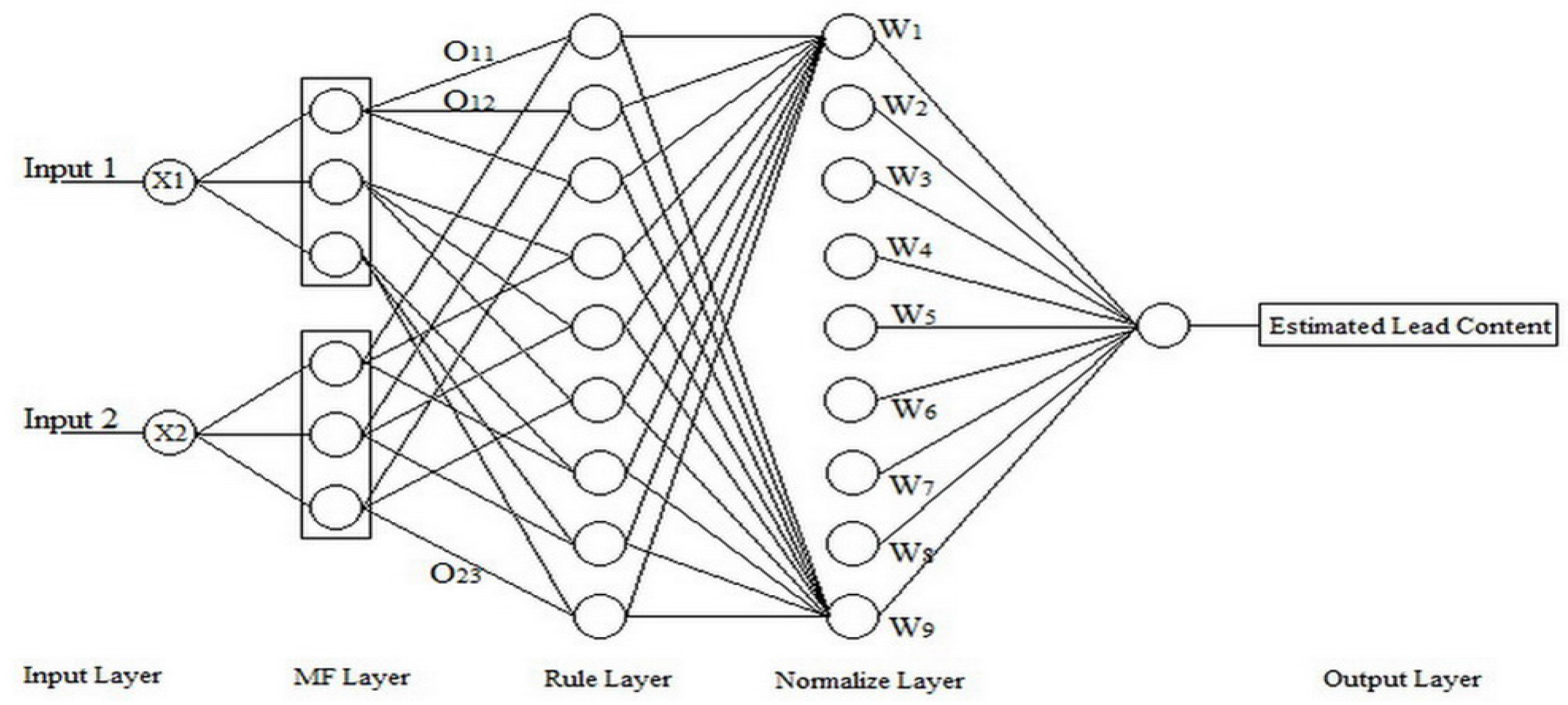
Figure 1. The structure of fuzzy neural network with two inputs and three membership functions.

Figure 1. The structure of fuzzy neural network with two inputs and three membership functions.

Neural networks and fuzzy systems are combined together to create fuzzy neural network [24,25]. The first report of a fuzzy neural network was presented by Takagi [26]. The fuzzy neural network presented in this research is based on the well-known Adaptive-Network-based Fuzzy Inference System (ANFIS) and the network is trained by a least square strategy [27]. Architecture of the implemented fuzzy neural network used in this study that applied two inputs and associated membership functions is shown in Figure 1.

Input parameters (X_i) are entered to the network from the input layer. The following network processes are described below. Here m is the number of input parameters and n shows the number of considered membership functions for each input parameter.

• Membership function layer

  $$O_{ij}^{(1)}=-\frac{{(X_i-a_{ij})}^2}{b_{ij}};i=1,2,\mathrm{...},m;j=1,\mathrm{..},n$$

  (4)
• Rule layer; where every possible combination of fuzzified inputs (membership values) are introduced to a fuzzy AND represented by the multiplication operator.

  $$\begin{array}{l}{O}_f^{(2)}=O_{ij}^{(1)}{O}_{kl}^{(1)}\\ i=1,2,\mathrm{...},m-1;k=i+1,\mathrm{..},m;j,l=1,2,\mathrm{..},n;f=1,2,\mathrm{...},r=\frac{1}{2}{n}^{2}m(m-1)\end{array}$$

  (5)
• Normalization layer

  $$O_f^{(3)}=\frac{O_f^{(2)}}{{\displaystyle \sum _{p=1}^r{O}_p^{(2)}}};f=1,2,\mathrm{...},r$$

  (6)
• Output layer

  $$O^{(4)}={\displaystyle \sum _{p=1}^r{O}_p^{(3)}}{W}_p$$

  (7)

In this network, a_ij and b_ij parameters, which are the mean and variance of Gaussian membership functions respectively are first initialized as the mean and variance of their corresponding input parameters. Then these parameters, as well as the weight of the output layer (w_i), are adjusted in the network training stage.

Weight parameters are determined via the least square method. For this reason O_i⁽³⁾ (i.e., the output of the normalization layer) are determined based on current values of a_ij, b_ij for all the training samples. Then weight parameters are determined to give the least square error in the output layer. When the weight w_i is determined, another least squared method is followed to find the a_ij and b_ij values of membership functions. Regarding non-linearity of the problem, Taylor expansion of the network output is considered and iteratively, corrections of a_ij and b_ij are determined. The process terminates when corrections become negligible [23].

2.3. Validation Parameters

The performance of the applied regression models are evaluated by the following most common criteria:

• Normalized Root Mean Squared Error (NRMSE); Normalizing the RMSE facilitates the comparison between datasets or models with different scales. Though there is no consistent means of normalization in the literature, the range of the measured data defined as the maximum value minus the minimum value is a common choice (Equation (8)).

  $$NRMSE=\frac{RMSE}{y_{\max }^{obs}-y_{\min }^{obs}}$$

  (8)

  where, y_max and y_min are the maximum and minimum values of the dependent variables [28].
• Coefficient of determination (R²); as a regression coefficient shows the goodness of fit between the observed and predicted values (Equation (9)).

  $$\begin{array}{c}{R}^2=1-\frac{S{S}_{res}}{S{S}_{tot}}\\ S{S}_{tot}={\displaystyle \sum _{i=1}^n{(y_i^{obs}-{\overline{y}}_i)}^2};S{S}_{res}={\displaystyle \sum _{i=1}^n{(y_i^{pre}-y_i^{obs})}^2}\end{array}$$

  (9)

  Where, SS_res is the summation of regression error and SS_tot is the summation of total error. R² ϵ [0, 1], when R² = 1 shows perfect correspondence between measured and predicted values. R² < 0.8 shows poor performance of the regression model [9].
• Ratio of Performance to Deviation (RPD); similar to R² describes the regression ability of a model (Equation (10)).

  $$RPD=\frac{SD(y^{obs})}{RMSE}$$

  (10)

  where, SD stands for standard deviation. RPD values of lower than 1.4 represent a poor model, while models with 1.4 < RPD < 2.1 are considered as acceptable models that need more improvement. Models with RPD > 2.1 are usually considered acceptable in most applications [9].

In this paper, subscripts C and V are used to show that these parameters are computed from control and validation (test) samples, respectively.

3. Study Area and Input Data

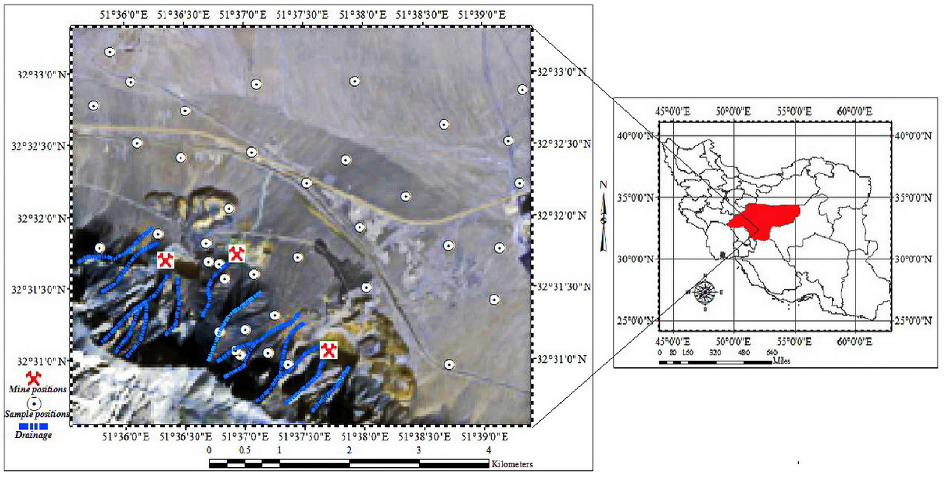
The study area was located in southern Isfahan, on the northern slopes of the Irankouh Mountains (Figure 2). Three mines were located in the area; one of them extracted from underground and the other two were active open pits.

Figure 2. Location of the case study area (Irankouh Mountains).

Figure 2. Location of the case study area (Irankouh Mountains).

The main rocks of study area are made of quartzes shale and sandstone from Jurassic era and dolomitic limestone of the cretaceous period. The mineral resources of the study area are minerals serosite, smithstonite, sphalerite, galena, calcite, barite and dolomite. The soil types in our study region were Entisol in USSD soil taxonomy [29] with the subgroup of Haplic Torriarents. These kinds of soils may have any mineral parent material, age, vegetation or moisture regime and any temperature regime. They do not have permafrost and the only features which are common to all soils of this order, are the absence of diagnostic horizons and the mineral nature of the soils. Torriarents are generally alkaline and many of them are calcareous. While the lead minerals in our investigation are galena and sphalrite whether, the Pb content of soil samples were carbonated and soil sampling was done from surface soils and the pure lead minerals did not have any direct effect on radio spectroscopy. The soils in our study have weak aridic moisture regime and the main of soil textures were sandy loam and loam. Due to existing carbonates in soil samples, pH values of studied soils were more than 7.5.

Additional information about this site can be found in [30].

Regarding that leaching and weathering of rocks releases heavy metals, soil Pb is usually concentrated in the drainages. This is the reason that the mines are approximately located at the converging end of drainages. Due to these points higher Pb variations was seen in the monotonous region surrounded by the three mines. This was also confirmed by the old available maps of the study area.

Due to the interpolative nature of regression techniques it was aimed to gather soil samples with a uniform distribution of the Pb concentrations values. According to higher variations of the Pb concentrations in the monotonous region a denser sampling was planned in this area. For this reason the mean sample distances of 150 m and 1 km were designed in the monotonous and field regions, respectively.

Generally the stratified systematic sampling strategy was followed in both regions although topographic situation imposed some limitations. In this probabilistic sampling strategy, the interest region is divided into smaller, regularly-spaced regions of a predefined size, and then a sample unit is chosen randomly from each of these regions (Figure 2).

For each sample, a 2 cm of the soil upper longer was gathered. Soil samples were then grained, followed by sifting and homologizing to detach any brushwood or coarse aggregate. 50 gram of each soil sample was sent to the laboratory for the determination of Pb concentrations using Inductively Coupled Plasma Atomic Emission Spectrometry (ICP-AES) with 1 ppm accuracy and Limit of Detection (LOD) equal to 0.5. ICP-AES, utilizing plasma as the atomization and excitation source, is known as a common successful analytical atomic spectroscopy method due to its sensitivity, good precision and accuracy as well as its fast preparation of samples [31]. Regarding the high numerical range of lead contents, logs were applied. Table 1 summarizes the general information of lead contents in the study area.

Table 1. Statistical parameters of soil Pb content in the study area.

Parameter	Mean (mg/kg)	Max (mg/kg)	Min (mg/kg)	SD (mg/kg)
Pb	1242.114	9797	60.36	2118.084

Table 1. Statistical parameters of soil Pb content in the study area.

Parameter	Mean (mg/kg)	Max (mg/kg)	Min (mg/kg)	SD (mg/kg)
Pb	1242.114	9797	60.36	2118.084

The remaining soil samples were used for spectrometry. Spectra Vista HR-1024i (Spectra Vista Co., New York, NY, USA) was used to measure spectrums of the samples. This spectrometer recorded spectral information from 350 nm to 2500 nm using three diodes: a silicon diode (350–1000 nm) that used 512 detectors and two Indium-Arsenic-Gallium diodes (1000–2500 nm) containing 256 detectors. The sampling resolution of this spectrometer was 1.5 nm, 3.8 nm and 9.5 nm in spectral ranges of 350–1000 nm, 1000–1890 nm and 1890–2500 nm respectively.

Before spectrometry, soil samples were sieved in 2 mm. In order to deal with the probable non-lambertian behavior of soil sample, the spectral reflectance of each one was measured from four different directions and then their mean was considered as the representative spectral reflectance curve.

Among the 38 samples, 28 were selected as control samples and the remaining 10 were kept as independent test samples. Control samples were used to solve the regression models, while the independent samples were only applied for performance evaluation of these models. The aim was to have uniform spatial and Pb value distributions for both the control and test sample set.

4. Results and Discussion

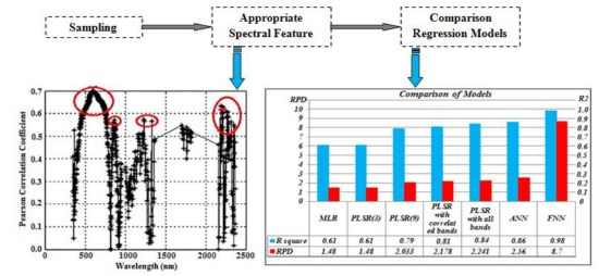
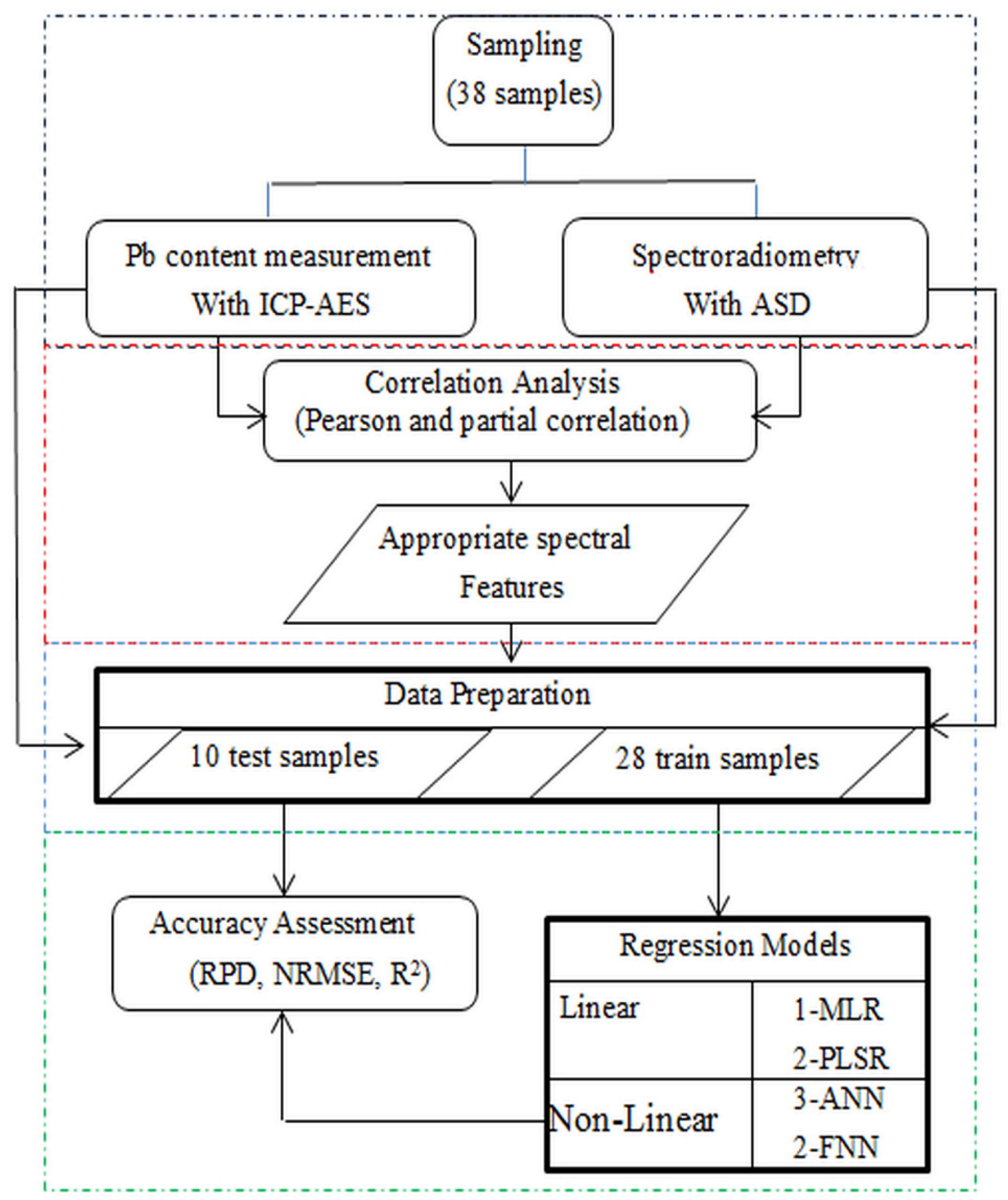
In the following, the appropriate extraction of spectral features is reported followed by implementation in linear and non-linear regression models. As mentioned before, MLP and PLSR were used for linear model evaluations and ANN and FNN were assessed for nonlinear regression comparison. Figure 3 shows the flowchart of the research.

Figure 3. Flowchart of research.

Figure 3. Flowchart of research.

4.1. Appropriate Spectral Features

Appropriate spectral features are commonly selected via a detailed study on their spectral behavior. This information may be found in spectroscopy text books such as [32]. However in this study we applied statistical tests to choose the appropriate spectral range and the most effective spectral regions. Then inspired by previous researches some candidate spectral features was extracted and the best ones were selected. In the following the details are presented.

At first, the aim was to design some appropriate spectral features from the observed spectral bands. For this reason at first the spectral bands centered on 950 nm, 1400 nm and 1900 nm were eliminated as the bands most highly effected by water absorption [33]. Then the correlation between the remaining spectral bands and the Pb concentrations was determined. This was done applying all 38 samples. 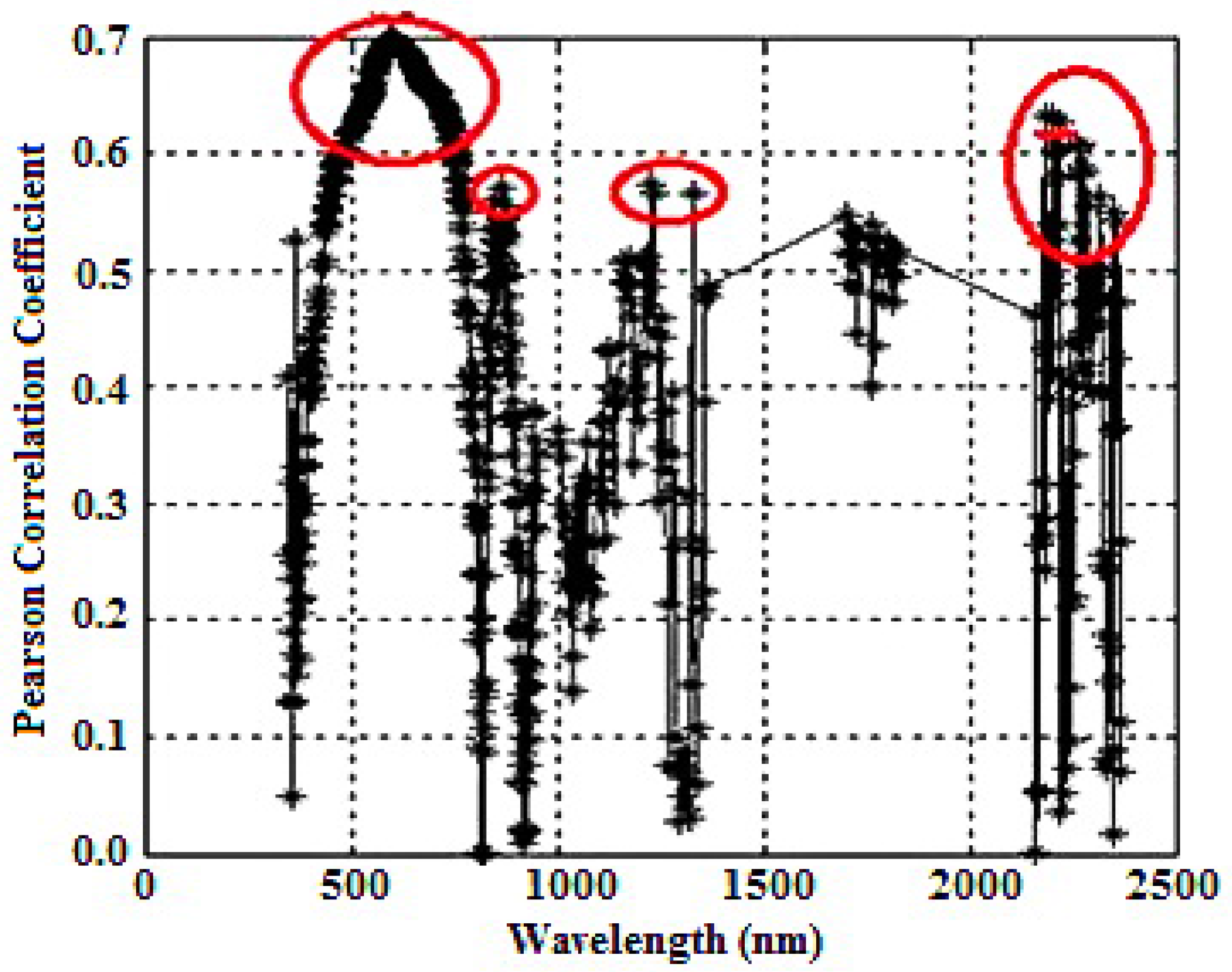Figure 4 shows the obtained results.

Figure 4. Correlation coefficient between different spectral bands and the Pb concentrations.

Figure 4. Correlation coefficient between different spectral bands and the Pb concentrations.

According to the above figures the most prominent correlation occurred in the visible spectral range (i.e., 450–750 nm) where correlation coefficient (as the measure of relationship strength between two variables) is higher than 0.6. The next correlated spectral range is 2170–2266 nm with correlation coefficients of above the 0.55. Two other local maximums are also seen centered at 860 nm and 1342 nm, where correlation coefficients are about 0.57.

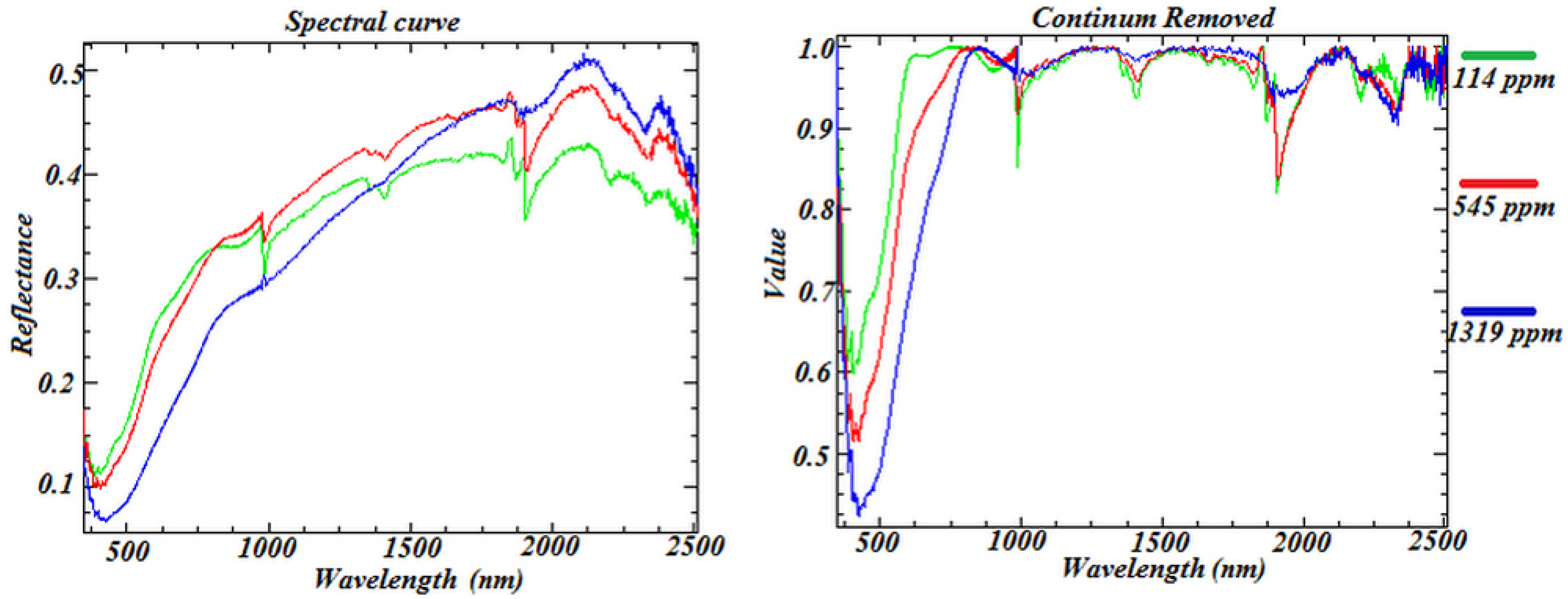
In the following, these correlated spectral ranges are considered as appropriate domains to design spectral features. The most common spectral preprocessing continuum removed [34,35,36] was implemented to eliminate the effect of spectral background and to provide a better indication of the absorption spectral ranges (Figure 5).

According to this figure, spectral areas centered on 410 nm, 860 nm, 1000 nm, 1342 nm and 2200 nm show absorption and therefore considered as effective spectral bands. In addition, the visible spectral areas centered on 375 nm, 500 nm and 610 nm, which are proposed in [3] and/or [7], are also considered as the most probable informative bands for spectral feature design.

Subsequently (R_375,610, R_410,610, R_500,610, R_610,860 and R_1000,1342) band ratios, (A₅₀₀, A₂₂₀₀) band areas and (D₅₀₀, D₂₂₀₀) absorbent depths are selected as candidates for the initial spectral features.

The correlation coefficient of these spectral features, with respect to the Pb concentrations was determined and then the significance test was performed at the probability level of p = 0.01 [17,37,38]. According to this investigation R_410,610, R_500,610 and D₂₂₀₀ with correlation coefficients of 0.25, 0.39 and 0.38, respectively, did not pass the significance test. In other words, it can be claimed (at 99% confidence level), that there was no meaningful relationship between these 3 features and the Pb concentrations, so they were eliminated from the list of candidates.

Figure 5. Continuum removed and spectral curves for samples with high lead content.

Figure 5. Continuum removed and spectral curves for samples with high lead content.

In order to consider the internal correlation of the candidate spectral features, partial correlation coefficient analysis was also performed [17,38]. In this analysis, all the candidate spectral features were set one-by-one as the control variable. The correlation coefficient of the remaining features was determined for to the Pb concentrations, eliminating the correlation effect of the selected control variable. Table 2 shows results of partial correlation analysis for the remaining 6 candidate spectral features.

Table 2. Results of partial correlation coefficient statistical analysis.

Control Variable	R375,610	R610,860	R1000,1342	D500	A500	A2200
None	0.530 *	0.794 *	0.733 *	0.634 *	0.770 *	0.530 *
R375,610	--	0.697 *	0.601 *	0.569 *	0.664 *	0.240
R610,860	0.051	--	0.028	0.101	0.032	0.059
R1000,1342	0.106	0.450	--	0.237	0.397	0.166
D500	0.437 *	0.463 *	0.510 *	--	0.49 *	0.469 *
A500	0.126	0.303	0.202	0.232	--	0.136
A2200	0.212	0.698 *	0.611 *	0.592 *	0.669 *	--

* Significant at p = 0.01.

Table 2. Results of partial correlation coefficient statistical analysis.

Control Variable	R375,610	R610,860	R1000,1342	D500	A500	A2200
None	0.530 *	0.794 *	0.733 *	0.634 *	0.770 *	0.530 *
R375,610	--	0.697 *	0.601 *	0.569 *	0.664 *	0.240
R610,860	0.051	--	0.028	0.101	0.032	0.059
R1000,1342	0.106	0.450	--	0.237	0.397	0.166
D500	0.437 *	0.463 *	0.510 *	--	0.49 *	0.469 *
A500	0.126	0.303	0.202	0.232	--	0.136
A2200	0.212	0.698 *	0.611 *	0.592 *	0.669 *	--

* Significant at p = 0.01.

A control variable is known as an appropriate and important feature if negligible and insignificant partial correlations are obtained for the other features [39]. Based on Table 1 R_610,860, R_1000,1342 and A₅₀₀ were selected as appropriate spectral features, which were then used in the following examined regression models.

4.2. Multiple Linear Regressions

Linear regression, as the simplest model, was implemented for the Pb concentration estimation from the spectral features. For this reason, the selected effective spectral features (i.e., R_610,860, R_1000,1342 and A₅₀₀) were first applied individually as independent variables and then all 3 were used together as input parameters. Table 3 shows the obtained validation parameters computed over both the control and test samples.

The RPD values, each of which was less than 2.1 indicate inefficiency of the simple regression model for the Pb concentration estimations. In this respect, the multivariable model (i.e., applying all 3 spectral features) showed no superiority against the one-variable models.

Table 3. Validation parameters for single- and multi-variable linear regression model.

Parameter	R610,830	R1000,1342	A500	R610,830 & R1000,1342 & A500
NRMSEc	0.157	0.168	0.168	0.15
RPDc	1.55	1.44	1.47	1.61
R2c	0.63	0.54	0.59	0.64
NRMSEv	0.198	0.216	0.214	0.198
RPDv	1.48	1.36	1.37	1.48
R2v	0.61	0.51	0.51	0.61

Table 3. Validation parameters for single- and multi-variable linear regression model.

Parameter	R610,830	R1000,1342	A500	R610,830 & R1000,1342 & A500
NRMSEc	0.157	0.168	0.168	0.15
RPDc	1.55	1.44	1.47	1.61
R2c	0.63	0.54	0.59	0.64
NRMSEv	0.198	0.216	0.214	0.198
RPDv	1.48	1.36	1.37	1.48
R2v	0.61	0.51	0.51	0.61

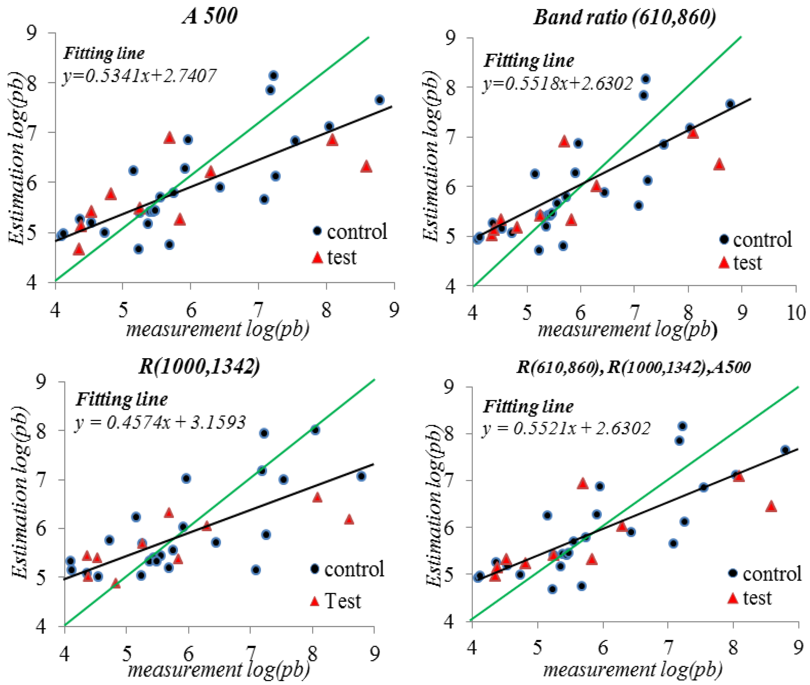
Figure 6 presents scatterplots of the Pb concentration estimations against the laboratory observed values for the control samples. In an ideal performance, it is expected that all the sample points plotted on the sector of axes. Accordingly the mismatch between the fittings line (black line) would indicate imperfection of the models. As shown in Figure 6, none of the MLR models showed promising performance for soil Pb estimation.

Figure 6. The scatterplot of estimations and expected the Pb concentration in simple linear regression model.

Figure 6. The scatterplot of estimations and expected the Pb concentration in simple linear regression model.

4.3. Partial Least Square Regression

Partial least-square regression (PLSR) transforms the independent and dependent variables into a new space of maximum correlation where different dimensions of this new space (e.g., factor number) can be applied. In the first investigation of this section, the previously selected spectral features (i.e., R_610,860, R_1000,1342 and A₅₀₀) were applied as input parameters and the model was named PLSR (3). In this model, all 3 possible factor numbers were evaluated. Table 4 shows the validation parameters computed over both the control and test samples.

Table 4. Evaluation criteria for PLSR (3).

Parameter	Factor 1	Factor 2	Factor 3
NRMSEc	0.152	0.149	0.149
RPDc	1.614	1.643	1.645
R2c	0.616	0.629	0.630
NRMSEv	0.206	0.200	0.199
RPDv	1.416	1.471	1.476
R2v	0.562	0.609	0.615

Table 4. Evaluation criteria for PLSR (3).

Parameter	Factor 1	Factor 2	Factor 3
NRMSEc	0.152	0.149	0.149
RPDc	1.614	1.643	1.645
R2c	0.616	0.629	0.630
NRMSEv	0.206	0.200	0.199
RPDv	1.416	1.471	1.476
R2v	0.562	0.609	0.615

According to Table 3, the best performance was achieved by the model with all 3 factors. However, this model was not appropriate according to RPD < 2.1.

In order to evaluate higher factor numbers and to consider the ability of PLSR to manage internal correlation of input parameters, all the 9 initial spectral features were used as the second experiment, termed as PLSR (9). Again all possible factor numbers were evaluated. Table 5 lists the evaluation criteria for this model.

Table 5. Evaluation criteria for PLSR (9).

Parameter	Factor 1	Factor 2	Factor 3	Factor 4	Factor 5	Factor 6	Factor 7	Factor 8	Factor 9
NRMSEc	0.202	0.152	0.759	0.149	0.146	0.134	0.119	0.126	0.126
RPDc	1.211	1.610	1.635	1.661	1.678	1.772	2.050	1.941	1.941
R2c	0.318	0.614	0.626	0.637	0.644	0.701	0.799	0.734	0.734
NRMSEv	0.225	0.210	0.206	0.214	0.226	0.152	0.144	0.157	0.155
RPDv	1.307	1.398	1.426	1.375	1.298	1.937	2.033	1.870	1.889
R2v	0.552	0.526	0.586	0.501	0.416	0.788	0.794	0.720	0.725

Table 5. Evaluation criteria for PLSR (9).

Parameter	Factor 1	Factor 2	Factor 3	Factor 4	Factor 5	Factor 6	Factor 7	Factor 8	Factor 9
NRMSEc	0.202	0.152	0.759	0.149	0.146	0.134	0.119	0.126	0.126
RPDc	1.211	1.610	1.635	1.661	1.678	1.772	2.050	1.941	1.941
R2c	0.318	0.614	0.626	0.637	0.644	0.701	0.799	0.734	0.734
NRMSEv	0.225	0.210	0.206	0.214	0.226	0.152	0.144	0.157	0.155
RPDv	1.307	1.398	1.426	1.375	1.298	1.937	2.033	1.870	1.889
R2v	0.552	0.526	0.586	0.501	0.416	0.788	0.794	0.720	0.725

Comparison between Table 3 and Table 4 showed that PLSR (9) performed better than PLSR (3) in factor numbers higher than 5. The best result by PLSR (9) was achieved in factor numbers of 7 where RPD = 2.033 was determined.

As another test, spectral information was also directly used in PLSR. In this practice once correlated bands and once all the available spectral bands were used as the independent variable of PLSR. Correlated bands were selected as those which passed the significance test of correlation coefficients with respect to lead content out the probability level of p = 0.01. In both cases different factors of PLSR are examined and the best ones are reported in Table 6.

As can be seen these two PLSRs achieved higher accuracy levels in comparison to those which applied the limited number of spectral features (i.e., PLSR (3) and PLSR (9)). However these models need the accessibility to all spectral information which is only available in hyperspectral images. Furthermore much more computational efforts were imposed as the numbers of independent variables were considerably increased.

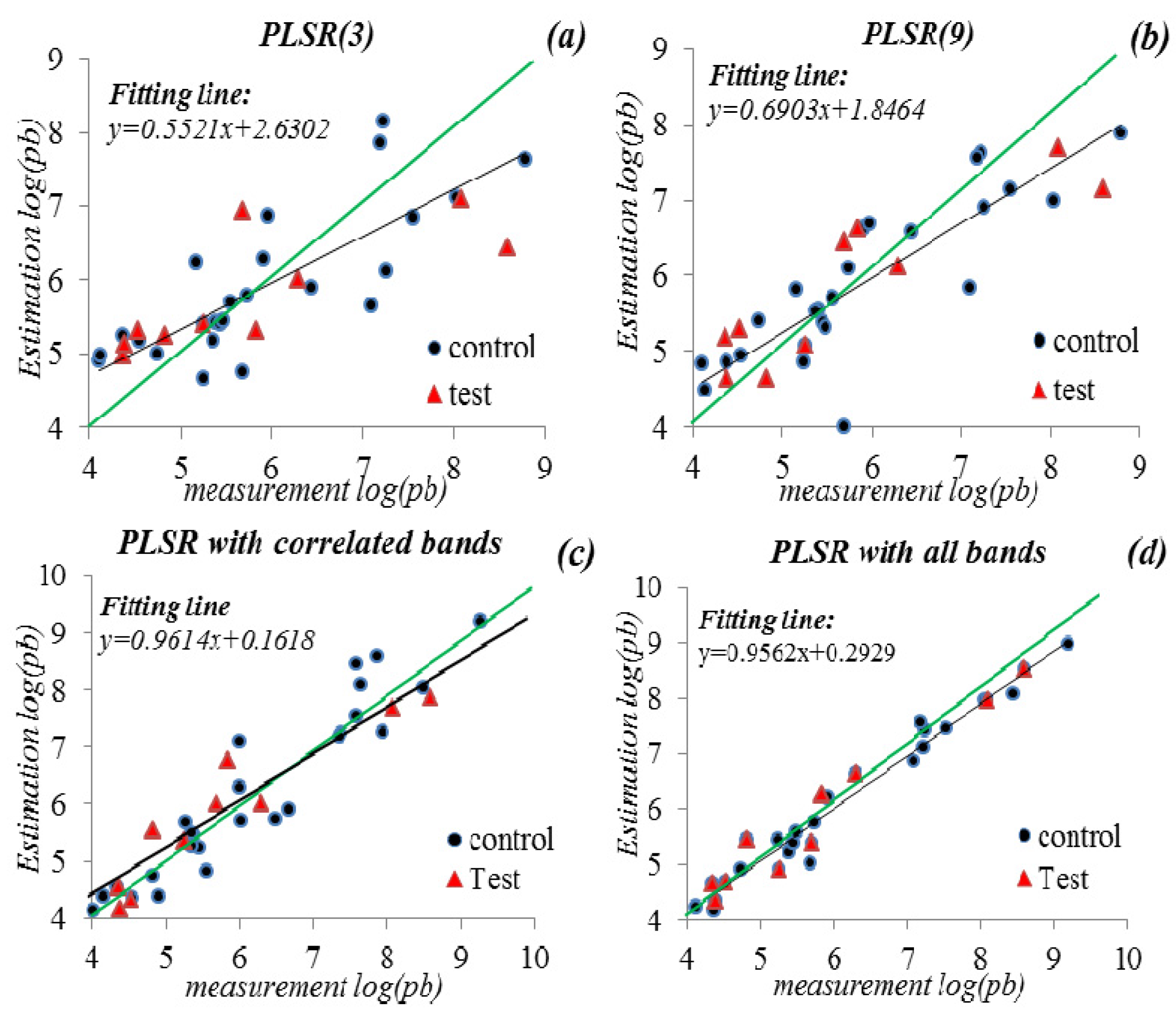
Figure 7 shows a scatterplot of these four models for test and control samples.

Figure 7. The scatterplot of estimated and expected the Pb concentration in (a). PLSR (3), (b). PLSR (9), (c). PLSR with correlated bands and (d). PLSR with all bands.

Figure 7. The scatterplot of estimated and expected the Pb concentration in (a). PLSR (3), (b). PLSR (9), (c). PLSR with correlated bands and (d). PLSR with all bands.

Table 6. Evaluation criteria for PLSR with correlated and all bands.

Method	NRMSEc	RPDc	R2c	NRMSEv	RPDv	R2v
PLSR with correlated bands (with 8 factor)	0.092	3.240	0.905	0.141	2.178	0.810
PLSR with all bands (with 9 factor)	0.054	5.514	0.967	0.137	2.241	0.844

Table 6. Evaluation criteria for PLSR with correlated and all bands.

Method	NRMSEc	RPDc	R2c	NRMSEv	RPDv	R2v
PLSR with correlated bands (with 8 factor)	0.092	3.240	0.905	0.141	2.178	0.810
PLSR with all bands (with 9 factor)	0.054	5.514	0.967	0.137	2.241	0.844

As can be seen PLSR is rather successful when a considerable number of independent variables (preferably direct spectral information) is available. However the limited number of spectral features could not be promising enough as the PLSR (9) could only achieve to RPD = 2.03.

4.4. Neural Network Model

A three layer feed forward neural network with tangent-sigmoid activation function was designed where the first layer received the input spectral features, the last layer presented the network response and the middle layer was in charge of the non-linear capability of the model.

Considering the selected 3 effective spectral features, 3 neurons were designed in the input layer while in the output layer only one neuron was set to represent the network response about the estimated Pb concentration. In the middle layer, different numbers of neurons were examined to determine the most appropriate level of non-linear behavior of the network.

A descending gradient algorithm was used for network training. From the 28 control samples 70% randomly selected ones were used as the training set and the remainders were applied as the internal validation set to avoid the problem of over fit.

Different numbers of neurons were tested in the middle layer and each network was trained 10 times to assess sensitivity of the network to the initial random parameters. Trained networks were implemented on the test samples and the computed validation parameters are presented in Table 7. Regarding the 10 successive runs for each network, the mean value and standard deviation of validation parameters are reported.

Table 7. Mean ± Standard Deviation (SD) criteria for 10 successive runs of different neural network.

Nu. of Middle Neurons	3	5	10	15	20
RMSE ± SD	1.271 ± 0.122	1.283 ± 0.264	1.069 ± 0.191	1.142 ± 0.388	1.350 ± 0.595
RPD ± SD	1.155 ± 0.102	1.177 ± 0.228	1.610 ± 0.415	1.416 ± 1.237	1.481 ± 1.133
R2 ± SD	0.298 ± 0.119	0.393 ± 0.142	0.524 ± 0.152	0.471 ± 0.424	0.400 ± 0.330

Table 7. Mean ± Standard Deviation (SD) criteria for 10 successive runs of different neural network.

Nu. of Middle Neurons	3	5	10	15	20
RMSE ± SD	1.271 ± 0.122	1.283 ± 0.264	1.069 ± 0.191	1.142 ± 0.388	1.350 ± 0.595
RPD ± SD	1.155 ± 0.102	1.177 ± 0.228	1.610 ± 0.415	1.416 ± 1.237	1.481 ± 1.133
R2 ± SD	0.298 ± 0.119	0.393 ± 0.142	0.524 ± 0.152	0.471 ± 0.424	0.400 ± 0.330

According to Table 7, the network with 10 neurons in the middle layer showed the best performance. However variations of network responses remained a concern. Table 8 shows the performance criteria for the best and worst networks containing 10 neurons in their middle layer.

Table 8. Validation criteria for the best and worst neural network with 10 neurons in the middle layer.

Parameter	Best	Worst
NRMSEv	0.11	0.23
RPDv	2.56	1.22
R2v	0.86	0.35

Table 8. Validation criteria for the best and worst neural network with 10 neurons in the middle layer.

Parameter	Best	Worst
NRMSEv	0.11	0.23
RPDv	2.56	1.22
R2v	0.86	0.35

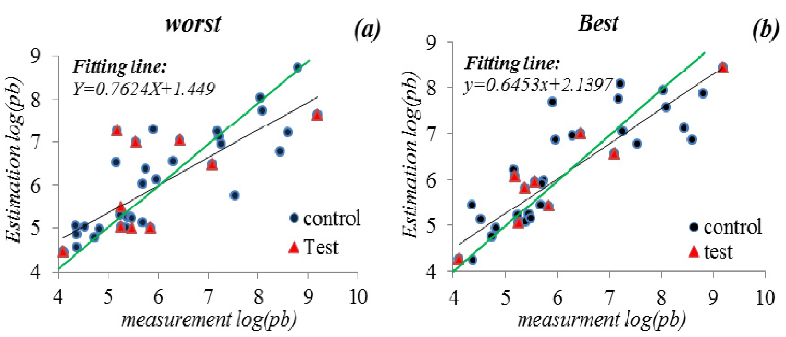
Although promising results were obtained from the best trained networks, there was a drawback of this non-linear regression model in that results were unstable and this contributed to considerable difference between best and worst trained networks. Figure 8 shows scatterplots for the worst and best neural networks.

Comparison between Figure 6 and Figure 8b, Figure 6 shows superiority of the neural networks. However considerable difference is shown between Figure 8a,b, this demonstrates an instability problem of neural networks and this is addressed in the section below.

Figure 8. The scatterplot of estimated and expected the Pb concentration in the worst (a) and best (b) neural networks.

Figure 8. The scatterplot of estimated and expected the Pb concentration in the worst (a) and best (b) neural networks.

4.5. Fuzzy Neural Network Model

Neural network models have adequate precision but instability in terms of results; this is because its responses are dependent on initial random weight parameters.

In order to solve this problem, the fuzzy neural network model (Section 2.2) was applied where the 3 selected effective spectral features (i.e., R_610,860, R_1000,1342 and A₅₀₀) were used as input parameters and different numbers of membership functions (MFs) were tested.

Trained networks were then implemented on the validation samples and the results are presented in Table 9.

Table 9. Validation criteria for different fuzzy neural networks.

Parameter	Nu. of MFs
	2	3	4
NRMSEc	0.160	0.006	3.31 × 10−6
RPDc	1.896	44.34	>50
R2c	0.786	0.999	1
NRMSEv	0.122	0.033	0.034
RPDv	2.012	8.761	8.396
R2v	0.828	0.988	0.984

Table 9. Validation criteria for different fuzzy neural networks.

Parameter	Nu. of MFs
	2	3	4
NRMSEc	0.160	0.006	3.31 × 10−6
RPDc	1.896	44.34	>50
R2c	0.786	0.999	1
NRMSEv	0.122	0.033	0.034
RPDv	2.012	8.761	8.396
R2v	0.828	0.988	0.984

Training by the least square technique, the fuzzy neural network does not need any initial random parameter assignment and thus obtains unique results for each data set.

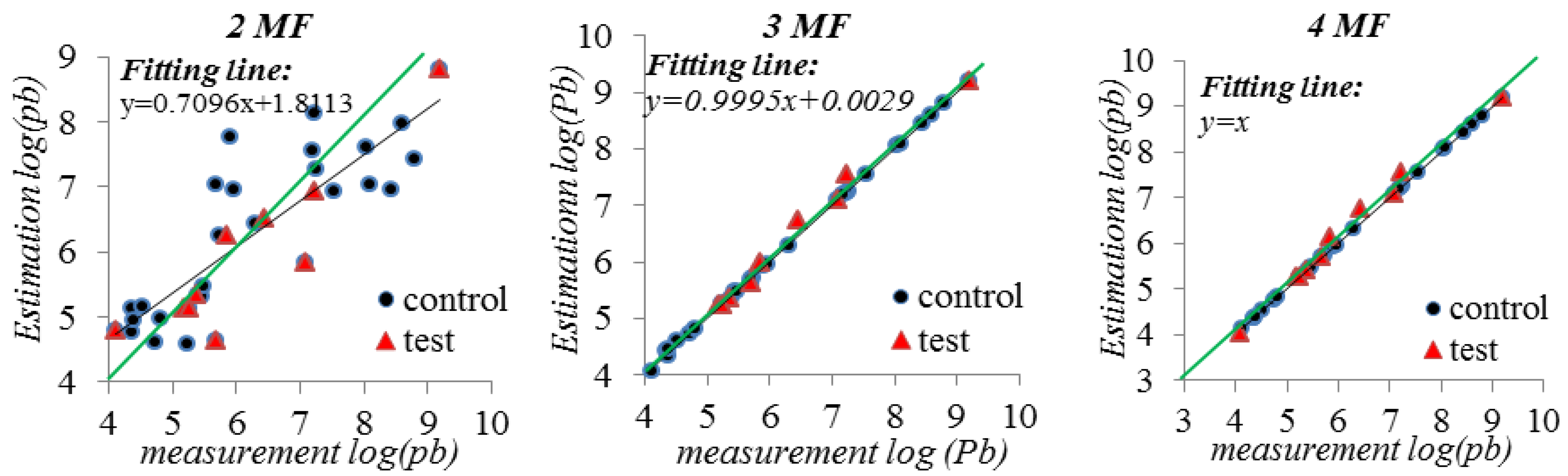
The results obtained demonstrate a high level of efficiency of the proposed FNN model for the prediction of the Pb concentration in soils from only 3 input spectral features. It also shows that MFs = 3 was the more accurate. It should be mentioned that if more than 4 MFs were to be used then there would be a lack of degree of freedom in the training stage. Figure 9 shows a scatterplot of the predicted Pb concentrations against expected values.

Figure 9. Scatterplot of measured and estimated lead amount with fuzzy neural network.

Figure 9. Scatterplot of measured and estimated lead amount with fuzzy neural network.

This Figure shows a high level match of the obtained results with estimated values for both of 3 MFs and 4 MFs.

Considering the possibility of land surface reflectance retrieval from the sensors mounted on aerial vehicles [40], the proposed FNN regression model is very promising for the production of accurate thematic maps of soil lead content from remotely sensed images.

5. Comparisons and Discussions

According to the investigations of Section 4.1, R_610,860, R_1000,1342, A₅₀₀, R_375,610, R_410,610, R_500,610, D₅₀₀, A₂₂₀₀ and D₂₂₀₀ were determined as the initial appropriate spectral features in soil lead content prediction where the first three ones are selected as the most effective. In comparison to [7], which proposed R_500,610 band ratio and D₅₀₀ band depth instead, although spectral areas centered on 500 nm and 610 nm are common, but in this research A₅₀₀ and R_610,860 are found to be more effective than D₅₀₀ and R_500,610 respectively. R_500,610 as the only independent variable of MLR achieved R² = 0.53 [7] in comparison to the proposed R_610,860 with R² = 0.61 in the same regression model (Table 3).

All three proposed spectral features were applied in the MLR model but unsatisfactory results were obtained with RDP = 1.48. The weakness of MLR for soil lead content prediction was also reported in [7]. This finding was also consistent with [13] where even the exploitation of 6 spectral features in MLR was not promising in lead content prediction purposes.

MLR was then replaced by the more advanced PLSR (3) model where again disappointing results with RPD = 1.48 was achieved. However utilization of all 9 initial spectral features could improve the PLSR (9) to high extent with RPD = 2.03. In comparison to [11] and [41], where in both spectral bands were directly used, the PLSR (9) was more precise. However the RPD < 2.1 indicated the need for more flexible regression models in soil lead content prediction from spectral information. Another drawback of the PLSR (9) was the need to the broader spectral range (i.e., 375–2200 nm) in order to extract its 9 input spectral features.

In the next attempt neural networks were verified as the non-linear regression models for soil lead prediction using again the only 3 most effective spectral features. In contrast to [9], which reported rather similar performances of PLSR and NNs in soil salt prediction, in this research NNs proved to be potentially superior than PLSR (9) as the best one achieved to RPD = 2.56. This is while instead of (375–2200 nm) required spectral range of PLSR (9), NNs used only 3 spectral features in (500–13500 nm).

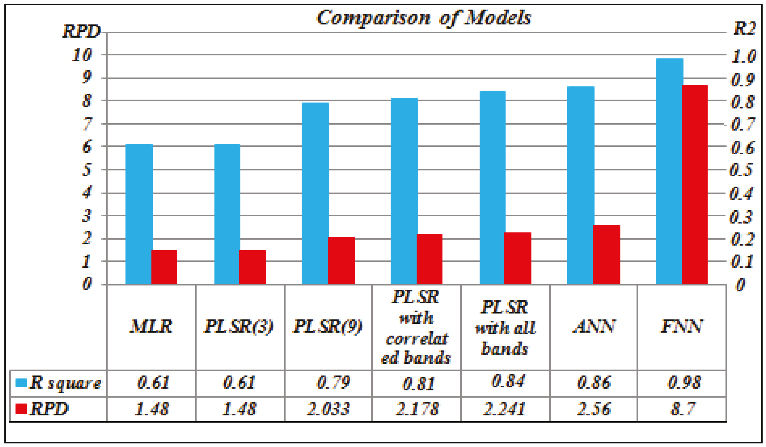
However instable performance was found as the main defect of NNs. The network training and functionality was highly affected by its initialization which caused different results in consequent runs. The problem was so severe that some poor NNs were even worse than MLR. Figure 10 gives a comparative perspective.

Figure 10. The comparison of different applied regression models in terms of R² and RPD.

Figure 10. The comparison of different applied regression models in terms of R² and RPD.

In order to deal with this problem, a Fuzzy Neural Network (FNN), introduced in Section 2.2, was used and verified. The proposed FNN showed high precise results with RPD = 8.76 which was much more promising than even the best neural network. Furthermore this FNN, benefited from a least squared based learning strategy, showed no evidence of instability problem.

6. Conclusions

The aim of this research was to design an accurate and reliable regression model for soil lead content estimation from a reflectance spectrum.

As the first achievement three spectral features were found as the effective independent variables including R_610,860 and R_1000,1342 band ratios and A₅₀₀ band area. This was done via the investigation of spectral behavior of a variety of lead containing soil samples followed by some statistical tests.

Designed spectral features were applied in both Multiple Linear Regression and Partial Least Square Regression models and it was discovered that these linear models are not flexible enough for soil lead content prediction from spectral features.

Neural networks, as the most well-known non-linear models, were then examined. It was found that neural networks can potentially predict soil lead contents with an acceptable accuracy as the best one achieved RPD = 2.56. However instability of results was found as the drawback of neural networks.

The most important achievement of this paper is proposing a kind of Fuzzy Neural Network (FNN) model for soil lead content prediction. The obtained results proved it high precise lead content prediction capability. Also being trained by a least squared strategy the proposed FNN benefits from full response stability.

The proposed FNN achieved RPD = 8.76 with only three input spectral features extracted from (500–1350 nm) spectral range. This spectral range is usually covered by most field/laboratory spectroradiometers as well as most airborne/space-borne remote sensing sensors. Accordingly the proposed FNN can be a very promising model for lead content thematic map production from remote sensing images. This is going to be the subject of our next research.