An Improved Method for Producing High Spatial-Resolution NDVI Time Series Datasets with Multi-Temporal MODIS NDVI Data and Landsat TM/ETM+ Images

Abstract

Due to technical limitations, it is impossible to have high resolution in both spatial and temporal dimensions for current NDVI datasets. Therefore, several methods are developed to produce high resolution (spatial and temporal) NDVI time-series datasets, which face some limitations including high computation loads and unreasonable assumptions. In this study, an unmixing-based method, NDVI Linear Mixing Growth Model (NDVI-LMGM), is proposed to achieve the goal of accurately and efficiently blending MODIS NDVI time-series data and multi-temporal Landsat TM/ETM+ images. This method firstly unmixes the NDVI temporal changes in MODIS time-series to different land cover types and then uses unmixed NDVI temporal changes to predict Landsat-like NDVI dataset. The test over a forest site shows high accuracy (average difference: −0.0070; average absolute difference: 0.0228; and average absolute relative difference: 4.02%) and computation efficiency of NDVI-LMGM (31 seconds using a personal computer). Experiments over more complex landscape and long-term time-series demonstrated that NDVI-LMGM performs well in each stage of vegetation growing season and is robust in regions with contrasting spatial and spatial variations. Comparisons between NDVI-LMGM and current methods (i.e., Spatial and Temporal Adaptive Reflectance Fusion Model (STARFM), Enhanced STARFM (ESTARFM) and Weighted Linear Model (WLM)) show that NDVI-LMGM is more accurate and efficient than current methods. The proposed method will benefit land surface process research, which requires a dense NDVI time-series dataset with high spatial resolution.

1. Introduction

The Normalized Difference Vegetation Index (NDVI) is one of the most commonly used vegetation indices to characterize the absorptive and reflective features of vegetation, which represent vegetation greenness and vigor [1,2,3]. Therefore, NDVI time-series data derived from multi-temporal satellite images are an appropriate data source for studying the spatial and temporal dynamics of ecosystem responses to climate change [4]. However, due to technological and budget limitations, there has been a trade-off within remote sensing instruments from high spatial resolution to more frequent coverage. Consequently, the available NDVI time-series products are generated from sensors with frequent observations (e.g., daily) but coarse spatial resolutions, ranging from 250 m to 8000 m, such as Moderate Resolution Imaging Spectroradiometer (MODIS) and NOAA Advanced Very High Resolution Radiometer (AVHRR). As a result, these products are incapable of capturing spatial details necessary for monitoring land cover and ecosystem changes in heterogeneous areas [5]. On the other hand, NDVI data derived from Landsat sensors (e.g., TM/ETM+/OLI with 30 meters resolution at visible and near infrared bands) can successfully capture the spatial details and alleviate the spectral mixture issue to some extent [6,7]. However, longer observation cycles of these satellites and frequent cloud contamination in some regions limit their application for detecting rapid changes in the ecosystem [8,9]. Combining NDVI data from multi-sensors is a possible solution for producing high spatial and temporal resolution NDVI data, which is a critical requirement for monitoring vegetation dynamics.

Since Landsat satellites and MODIS have similar orbital parameters and less than 30 minutes difference in crossing time, methods have recently been developed and validated for blending Landsat TM/ETM+ and MODIS data [10,11,12,13]. Generally, there are two strategies to generate a fine-spatial resolution NDVI data from MODIS time series with the help of Landsat data. The first one is the indirect strategy, in which fine spatial-resolution NDVI is calculated from the reflectance data downscaled from MODIS data [14,15]. Up to now, there are many algorithms developed for downscaling MODIS reflectance with the help of fine-resolution sensor imagery. These algorithms include the Spatial and Temporal Adaptive Reflectance Fusion Model (STARFM) [10], the Spatial Temporal Adaptive Algorithm for mapping Reflectance Change (STAARCH) [11], the Semi-physical Fusion Approach [16], the Enhanced STARFM (ESTARFM) [13], the multi-temporal fusion method [17], and the Spatial Temporal Data Fusion Approach (STDFA) [18]. These methods can be categorized into two groups. STARFM, STAARCH, the Semi-physical Fusion Approach, and ESTARFM belong to the first group, which obtains the relationship of reflectance between MODIS and Landsat data from one or more pairs of images. Then this relationship is used to predict Landsat-like reflectance from MODIS data at prediction dates. The drawbacks for these methods are: (1) they often require known image pairs as close as possible to the prediction dates because the relationship between MODIS and Landsat learned from known pairs may change with time; and (2) they often have more strict assumptions when deducing the relationship between MODIS and Landsat, and these assumptions may not valid in reality. For example, STARFM assumes Landsat pixels within one MODIS pixel have the same change, while ESTARFM assumes that reflectance of each land cover has a linear change between two known dates. The second group is the unmixing-based methods, including the multi-temporal fusion method and STDFA. These algorithms predict fine-resolution reflectance from MODIS using the linear unmixing techniques, in which the fractional cover of each endmember is provided by Landsat or other ancillary data [19]. The multi-temporal fusion method employs a soft clustering method to address the intra-class variability issue. However, considering that soft clustering is not a mature technology, the errors from soft clustering introduce extra uncertainties for predicting fine-resolution reflectance. For STDFA, it only used two Landsat data (the beginning and end date of the prediction period) to estimate fractional cover. This would lose important temporal change information and lead to an inappropriate cluster result. Besides, it generated synthetic Landsat data by adding temporal changes to original data, while temporal changes were obtained from the reflectance unmixed from the MODIS data at two dates. During this procedure, errors from two spectral unmixing steps would aggregate to the final predictions. Additionally, most of the current unmixing based methods only use fine-resolution data to provide fraction information, while other important information including spatial details are missing in these methods. More important, indirect approaches, regardless of what reflectance blending algorithms used, all suffer from heavy computation loads and errors accumulation, because both reflectance of red and NIR bands must be predicted before calculating NDVI. A recent study using three sites with contrasting spatial and temporal heterogeneity has demonstrated this limitation for nine indices including NDVI [15]. It compares the prediction results of using the indirect approaches and the ones of directly downscaling NDVI using the blending algorithms (e.g., STARFM, ESTARFM), and concludes that directly downscaling NDVI would get better results than indirect strategy [15].

The second strategy is to directly downscale the NDVI product, which could directly apply blending algorithms from the first strategy or use methods specifically developed for blending NDVI as well. Busetto et al. proposed a novel approach for directly downscaling MODIS NDVI based on a Weighted Linear Mixing model (WLM) [20,21], which assumes that the NDVI value of a coarse pixel can be calculated as the area fraction weighted average of NDVI values of several land cover classes at a fine spatial scale within the coarse pixel [22]. However, its basic assumption that the same land cover type has the same NDVI value is somewhat unreasonable in the real situations, because spectral variability is very common in the same land cover type, especially within larger areas [23]. Such unreasonable assumption is likely to cause large estimation errors and significant loss of spatial details. Recently, a Spatial and Temporal Adaptive Vegetation index Fusion Model (STAVFM) was also developed based on STARFM to directly downscale MODIS NDVI with the help of HJ-1 images, which include four spectral bands with similar characteristics (i.e., spatial resolution, band width, spectral response functions) with band 1–4 of Landsat TM sensor [24]. To modify the original STARFM model, STAVFM defines a time window based on expert knowledge about crop phenology, which was then used to choose more appropriate data pairs for the blending process. However, the specification of crop phenology limits its applications to other regions. Therefore, the main challenge remains of directly downscaling NDVI products with higher accuracy and fewer requirements of ancillary data or prior knowledge.

In order to address limitations of current methods for directly downscaling NDVI from MODIS, we developed the NDVI Linear Mixing Growth model (referred to hereafter as NDVI-LMGM) to directly obtain NDVI time-series data with a high spatial resolution. The main goal of the proposed approach is to achieve more accurate results but with less computational costs and prior knowledge through using the spatial details from acquired Landsat images. To test the effectiveness of the proposed approach, we compared it to several other typical and popular methods, including STARFM [10], ESTARFM [13], and WLM [22].

2. Methodology

2.1. The Theoretical Basis

Although the temporal change of NDVI is complicated due to the intricate dynamics of vegetation growth, the short-term changes can be interpreted as linear. This assumption is reasonable because the continuous change curve of NDVI can be separated into several linear segments (Figure 1). The relationship of NDVI between two different points in time, t₁, t₂, can be denoted in Equation (1):

$$NDV{I}_2=NDV{I}_1+k\times (t_2-t_1)$$

(1)

where NDVI_i is the NDVI value of a date t_i, and k represents the corresponding growth rate from t₁ to t₂. Equation (1) provides an opportunity to obtain the NDVI at the predicted date via the growth rate during a particular period and one NDVI observation (base observation) if they are known beforehand.

Figure 1. Schematic diagram of a NDVI growth curve and its linear segments.

Figure 1. Schematic diagram of a NDVI growth curve and its linear segments.

The MODIS growth rate between any two dates can be calculated using MODIS NDVI time-series data (e.g., MOD13 16-day composite product). Accordingly, how to estimate the growth rate for each TM/ETM+ pixel from the growth rate at the MODIS scale becomes a key problem to obtain the Landsat-like NDVI value for a prediction date. A linear mixing model was employed to solve the problem, although it was strictly valid only for the original reflectance values [25]. In the last decades, research has demonstrated that this linear mixing model would introduce very small errors to statistics when replacing the reflectance by NDVI (Equation (2)) [15,21,26].

$$NDVI\text{(}x,y,t\text{)}={\displaystyle \sum _{c=1}^l{f}_c\text{(}x,y,t\text{)}\times NDV{I}_c\text{(}x,y,t\text{)}}+\epsilon \text{(}x,y,t\text{)}$$

(2)

where NDVI(x, y, t) is the NDVI value of a MODIS pixel (x, y) at time t, f_c(x, y, t) and NDVI_c(x, y, t) represents the fractional coverage and the NDVI value of land cover class C within the MODIS pixel (x, y) at time t, respectively, l is the total number of land cover classes in the MODIS pixel (x, y) and ε(x, y, t) is the error term introduced by the Linear Mixing model.

When Equation (2) is applied to Equation (1), the relationship between the growth rate of a MODIS pixel and the corresponding TM/ETM+ pixels can be written as Equation (3), assuming that no land cover changes occur from t₁ to t₂ (See the supplementary materials for Equation (3)):

$$k^{MODIS}(x,y,t_1\to t_2)={\displaystyle \sum _{c=1}^l{f}_c(x,y,t_1)\times k_c^{TM}(x,y,t_1\to t_2)}$$

(3)

where k^MODIS (x, y, t₁→t₂) is the growth rate of a MODIS pixel (x, y) from t₁ to t₂, k_c^TM(x, y, t₁→t₂) is the growth rate of land cover C on the TM/ETM+ pixel scale within the corresponding MODIS pixel from t₁ to t₂. Equation (3) makes it possible to derive the growth rate of a land cover class on the TM/ETM+ pixel scale from the corresponding MODIS pixel if the f_c(x, y, t) values of all land cover classes within the MODIS pixel have been established.

Usually, there is more than one land cover class within a MODIS pixel, which means the unknown parameters k_c^TM(x, y, t₁→t₂) (c = 1, … , l) cannot be estimated unless at least l or more equations are available. Therefore, the spatially neighboring MODIS pixels are employed to provide extra information, assuming the same land cover class has a similar growth rate among these neighboring pixels. It is well known that vegetation growth represented by a change in NDVI is determined by vegetation type and natural growing conditions (i.e., climate, soil and nutrition conditions). For small areas, it is reasonable to assume that these natural growing conditions would be similar. Accordingly, the same land cover class with a similar vegetation type can be assumed to have a similar growth rate among the neighboring pixels. Thus, the neighboring pixels can be used to obtain a linear model system with the general matrix equation, as shown below:

$$\left[\begin{array}{c}{k}^{MODIS}(1,1,\text{Δ}t)\\ ⋮\\ k^{MODIS}(x,y,\text{Δ}t)\\ ⋮\\ k^{MODIS}(n,n,\text{Δ}t)\end{array}\right]=\left[\begin{array}{cccc}{f}_1(1,1)& f_2(1,1)& \cdots & f_l(1,1)\\ ⋮& ⋮& & ⋮\\ f_1(x,y)& f_2(x,y)& \cdots & f_l(x,y)\\ ⋮& ⋮& & ⋮\\ f_1(n,n)& f_2(n,n)& \cdots & f_l(n,n)\end{array}\right]\left[\begin{array}{c}{k}_1^{TM}(x,y,\text{Δ}t)\\ ⋮\\ k_c^{TM}(x,y,\text{Δ}t)\\ ⋮\\ k_l^{TM}(x,y,\text{Δ}t)\end{array}\right]$$

(4)

where Δt denotes the time difference from date t₁ to t₂; k^MODIS (x, y, Δt) and f_c(x, y) in Equation (4) can be calculated from the MODIS time-series data and the Landsat TM/ETM+ data, respectively. Then, k_c^TM(x, y, Δt) can be easily estimated by solving these linear equations. Subsequently, the estimated growth rates of various land cover classes on the TM/ETM+ scale can be used in Equation (1) to predict the NDVI value of t₂.

According to the assumption that the short-term change of NDVI is linear, all the equations mentioned above are reasonable. However, in the long run, the NDVI change will cease to follow a linear change pattern. Therefore, long-term NDVI change can only be predicted reliably by several short-term predictions. Specifically, for three successive dates (e.g., t_m is the Landsat observation date, t_m+1, t_m+2 are two prediction dates and t_m < t_m+1 < t_m+2), the NDVI prediction for t_m+2 at TM/ETM+ scale could be calculated using the following equation by assuming that the NDVI changes between t_m, t_m+1 and t_m+1, t_m+2 are linear, respectively,

$$NDV{I}_{m+2}=NDV{I}_m+k_m\times (t_{m+1}-t_m)+k_{m+1}\times (t_{m+2}-t_{m+1})$$

(5)

where NDVI_m and NDVI_m+2 are the NDVI value at t_m and t_m+2 at TM/ETM+ scale, k_m and k_m+1 are the growth rate at the TM/ETM+ scale from t_m to t_m+1, and t_m+1 to t_m+2, respectively.

2.2. Algorithm Implementation

The input data required for this proposed algorithm includes the MODIS NDVI time-series data (either the MOD13 vegetation index product or the NDVI data derived from the daily reflectance product (MOD09)) and at least one Landsat TM/ETM+ image. A flowchart of the proposed algorithm, shown in Figure 2, can be used to finally obtain high spatial-resolution NDVI time-series data. The main steps of implementation will be explained in detail in the following sections.

Figure 2. The flowchart of NDVI Linear Mixing Growth model (NDVI-LMGM).

Figure 2. The flowchart of NDVI Linear Mixing Growth model (NDVI-LMGM).

2.2.1. Data Pre-Processing

It is best to employ cloud-free Landsat TM/ETM+ images as the input data. However, to some extent, cloud contamination is an inevitable problem for the Landsat data acquisitions [27]. Alternatively, the Landsat TM/ETM+ images with an acceptable amount of cloud coverage can be used as possible input data after the cloudy areas are filled in by the NSPI method proposed by Zhu et al [28]. After that, Landsat TM/ETM+ images are geo-registered to MODIS NDVI image and orthorectified using the automated registration and orthorectification package (AROP) [29]. Digital numbers are then calibrated and atmospherically corrected using the Landsat Ecosystem Disturbance Adaptive Processing System (LEDAPS) [30]. Finally, NDVI images at the Landsat TM/ETM+ scale are calculated from the processed Landsat TM/ETM+ images. Similar to the Landsat data, it is possible that the MODIS NDVI time-series data could be obscured by cloud contamination [31]. To reduce the influence of the cloud contamination, MODIS NDVI time-series data is filtered using the Savitzky–Golay algorithm [32]. In addition, if NDVI data derived from the daily reflectance product (MOD09 at a spatial resolution of 250 m) is used, the deconvolution method proposed by Huang et al. can be employed to reduce errors introduced by the spatial response function of MODIS sensor [33,34].

2.2.2. Land Cover Classification Using LANDSAT TM/ETM+ Images

The land cover classification on the Landsat TM/ETM+ scale must be determined in advance so that f_c(x, y) can be calculated. Previous studies have used highly accurate high spatial-resolution land cover maps to obtain f_c(x, y) [22]; however, such maps are not always available for all areas. For the new method, the land cover map can be obtained by classifying all available Landsat TM/ETM+ images. To keep the new method as automated as possible, an unsupervised classification method (i.e., ISODATA) is recommended because it can achieve relatively accurate classification results with less human intervention. It should be noted that associating each class with the true land cover types (i.e., barren land, forest, etc.) when using the unsupervised classification result is not required. Since multi-temporal Landsat TM/ETM+ data can improve classification accuracy [35,36], it is best to collect as much Landsat TM/ETM+ data covering the study area as possible for land cover classification. Users must empirically set parameters of the numbers of classes in the ISODATA, the value of which can be determined according to the complexity of the landscape in the study area by visual evaluation of the input Landsat images. Greater complexity of the landscape requires establishing more class numbers. How the setting of the class numbers affects the performance of the new method will be discussed in the Section 4.2.

2.2.3. Predict Fine-Resolution NDVI

Theoretical analysis has shown that the computation of the TM/ETM+ NDVI growth rates requires at least l MODIS pixels since there are l parameters to be estimated (see Equation (4)). The selection of spatially neighboring MODIS pixels was performed via a moving window on a MODIS image (Figure 3). To ensure that a sufficient number of these were selected for solving the linear system, and that the window size satisfied the condition presented in Equation (6),

$$s\ge (\sqrt{l}-1)/2$$

(6)

where 2s + 1 is the moving window size and l is the number of classes.

Figure 3. The spatially neighboring pixels of a target MODIS pixel in a moving window and land cover composition in a MODIS pixel classified from available TM/ETM+ images.

Figure 3. The spatially neighboring pixels of a target MODIS pixel in a moving window and land cover composition in a MODIS pixel classified from available TM/ETM+ images.

Then the linear system in Equation (4) can be solved by a constrained least square method with upper and lower boundaries for the variable k_c^TM, presented in the equation below,

$$k_{\min }^{MODIS}-STD\left(k^{MODIS}\right)\le k_c^{TM}\le k_{\max }^{MODIS}+STD\left(k^{MODIS}\right)$$

(7)

where STD(k^MODIS), k_min^MODIS and k_max^MODIS are the standard deviation as well as the minimum and maximum values of the MODIS growth rate for the entire study area. This constraint is used to avoid the unreasonable large or small growth rates retrieved from Equation (4), which may be caused by errors and noise in classification of Landsat images or MODIS time-series data.

The next step was to obtain the fine-resolution growth rates from the procedures discussed above. Equation (1) was used to calculate fine-resolution NDVI of the prediction date t₂ with the help of fine-resolution NDVI from the observation date t₁. Moreover, if there are two available fine-resolution NDVI images from different observation dates (i.e., t_1,m, t_1,n), both of which can be used as the base NDVI observation in Equation (1), a weighted combination procedure can be employed to integrate the two prediction results P_m and P_n to produce a final prediction, as shown in Equation (8):

$$P=w_m{P}_m+w_n{P}_n$$

(8)

$$w_k=\frac{1/\left|{\displaystyle \sum _{i=1}^{N}NDV{I}^{MODIS}(x_i,y_i,t_{1,k})}-{\displaystyle \sum _{i=1}^{N}NDV{I}^{MODIS}(x_i,y_i,t_2)}\right|}{{\displaystyle \sum _{k=m,n}1/\left|{\displaystyle \sum _{i=1}^{N}NDV{I}^{MODIS}(x_i,y_i,t_{1,k})}-{\displaystyle \sum _{i=1}^{N}NDV{I}^{MODIS}(x_i,y_i,t_2)}\right|}}$$

(9)

where w_k is the weight of the observation date t_1,k (k = m, n), which is calculated according to the change magnitude detected from MODIS NDVI time series between the observation date t_1,k (k = m, n) and the prediction date t₂. Here, N is the MODIS pixel number in each moving window for which the weight is specified. Equation (9) assigns a more substantial weight to a NDVI prediction if fewer changes occurred between the prediction date and the observation date [13].

3. Experiments and Results

3.1. Study Area and Test Data

In order to test the performance of the proposed method, NDVI-LMGM, three typical methods for downscaling MODIS NDVI with the help of Landsat TM/ETM+ imagery were selected for comparison, ESTARFM, STARFM and the WLM. In previous studies, STARFM’s performance in blending reflectance data has been demonstrated to be inferior to that of ESTARFM, especially in heterogeneous landscapes [13]. If we assume NDVI at coarse resolution is a linear mixture of NDVI at fine resolution, this will fit the basic assumption of STARFM. Therefore, we can apply STARFM directly to downscale NDVI. To avoid redundant comparisons, this study only applied STARFM to directly blend MODIS NDVI and Landsat NDVI data rather than reflectance data.

To fairly compare the proposed method with both STARFM and ESTARFM, we employed the preprocessed satellite data from the same forest region with ESTARFM and STARFM’s experiments. The size of the study area is 400 × 400 pixels on the TM/ETM+ scale, and it is located approximately 37.5°N and 77.1°W. In this study area, the growing season is short and phenology changes rapidly [10,13]. Three pairs of Landsat-7 ETM+ and MODIS (MOD09) reflectance images were acquired on 24 May 2001, 11 July 2001 and 12 August 2001, respectively (Figure 4).

Figure 4. The MODIS (upper) and Landsat ETM+ (lower) images in a forest region (NIR-red-green composite and identical linear stretch).

Figure 4. The MODIS (upper) and Landsat ETM+ (lower) images in a forest region (NIR-red-green composite and identical linear stretch).

It must be noted that the above test site may be too small to draw comprehensive and credible conclusions from the comparison. Therefore, these four methods were also quantitatively compared in two larger areas with varying land surface characteristics, i.e., the Coleambally Irrigation Area and the Lower Gwydir Catchment, both located in Australia. These two areas have been used to evaluate blending algorithms, including STARFM and ESTARFM, in previous studies [37]. The Coleambally Irrigation Area (referred to as ‘Coleambally’ hereafter) is dominated by paddy fields and includes an irrigation system, located in southern New South Wales (34.6°S, 145.6°E, 1720 × 2040 pixels at 25-m resolution for ETM+ data). A total of 17 cloud-free pairs of Landsat-7 ETM + and MODIS reflectance images (MODIS Terra MOD09GA collection 5) were collected in this area (Figure 5a–d), covering the growing season from October 2001 to May 2002. The Coleambally area was selected because of its spatially heterogeneous landscape [37].

Figure 5. Sample pairs of ETM+ and MODIS data acquired at prediction dates (a) 16 October 2001, (b) 3 December 2001, (c) 21 February 2002, and (d) 17 April 2002 (NIR-Red-Green composite and identical linear stretch); and (e) the ETM+ NDVI time-series for Coleambally and irrigated area, respectively. All prediction dates are marked by the red dotted frames.

Figure 5. Sample pairs of ETM+ and MODIS data acquired at prediction dates (a) 16 October 2001, (b) 3 December 2001, (c) 21 February 2002, and (d) 17 April 2002 (NIR-Red-Green composite and identical linear stretch); and (e) the ETM+ NDVI time-series for Coleambally and irrigated area, respectively. All prediction dates are marked by the red dotted frames.

Another study area was the Lower Gwydir Catchment (referred to as “Gwydir” hereafter), located in northern New South Wales (28.9°S, 149.3°E, 3200 × 2720 pixels at 25-m resolution for ETM+ data). A total of 14 cloud-free pairs of Landsat-5 TM and MODIS reflectance images (MODIS Terra MOD09GA collection 5) were collected (Figure 6a–d)), approximately covering the entire year from April 2004 to April 2005. Notably, a large flood struck Gwydir in December 2004, which inundated nearly 44% of the entire area (Figure 6d). Therefore, Gwydir was classified as a temporally heterogeneous region [37]. More detailed information about data pre-processing can be found in previous studies [37].

In addition, another test area with a larger area (34.5°N, 109°E, 6140 × 6053 pixels at Landsat scale) and more temporal observation points, Xi’an City (Shanxi Province, China, Figure 7), was selected to qualitatively assess the effectiveness of the proposed method. The multi-temporal MODIS NDVI product (16-day, MOD13) depicting the entire year of 2009 was downloaded from NASA (http://earthdata.nasa.gov/) along with corresponding Landsat TM images acquired on 21 January, 30 June, and 5 November 2009, respectively.

Figure 6. Sample pairs of Landsat-5 TM and MODIS data acquired at prediction dates (a) 2 May 2004, (b) 25 October 2004, (c) 12 December 2005, and (d) 13 January 2005 (SWIR-NIR-Red composite and identical linear stretch); and (e) the TM NDVI time-series of entire Gwydir and flooded area. All prediction dates are marked by red dotted frames.

Figure 6. Sample pairs of Landsat-5 TM and MODIS data acquired at prediction dates (a) 2 May 2004, (b) 25 October 2004, (c) 12 December 2005, and (d) 13 January 2005 (SWIR-NIR-Red composite and identical linear stretch); and (e) the TM NDVI time-series of entire Gwydir and flooded area. All prediction dates are marked by red dotted frames.

Figure 7. The location of the test area (Xi’an City, Shanxi Province, China) and its corresponding of Landsat TM image (NIR-red-green composite).

Figure 7. The location of the test area (Xi’an City, Shanxi Province, China) and its corresponding of Landsat TM image (NIR-red-green composite).

3.2. Performance Comparison of Four Methods over a Small Forest Region

Considering that ESTARFM and WLM both require at least two pairs of Landsat TM/ETM+ and MODIS images to estimate the reflectance/NDVI on the prediction date. We also used two pairs of NDVI-LMGM and STARFM as inputs for an equitable comparison. We selected 11 July 2001 as the prediction date and two pairs of Landsat-7 ETM + and MODIS data acquired on 24 May and 12 August 2001 as inputs. The available actual Landsat ETM+ image from 11 July was further used as a reference to evaluate the accuracy of the prediction results. The class number of NDVI-LMGM was set as four classes (same with STARFM and ESTARFM in [10,13]), and the moving window size was 3 × 3 according to Equation (6), excluding the edge pixels. Figure 8 shows the NDVI predictions from July 11, 2001 at the TM/ETM+ scale according to the four methods. It is evident that the NDVI images predicted by NDVI-LMGM (Figure 8a), ESTARFM (Figure 8b) and STARFM (Figure 8c) are comparable; all are highly similar to the actual NDVI image directly calculated from the original Landsat ETM+ image (Figure 8e). These three predictions seem much more accurate than the result obtained from the WLM method (Figure 8d).

In order to quantify the accuracy assessment, the Average Absolute Difference (AAD, Equation (10)), Average Absolute Relative Difference (AARD, Equation (11)) and Average Difference (AD, Equation (12)) between the predicted and the actual NDVI values were calculated using the four methods (Table 1).

$$AAD=\frac{1}{n}{\displaystyle \sum _{i=1}^n\left|NDV{I}_i^p-NDV{I}_i^o\right|}$$

(10)

$$AARD=\frac{1}{n}{\displaystyle \sum _{i=1}^n\left|\left(NDV{I}_i^p-NDV{I}_i^o\right)/NDV{I}_i^o\right|}$$

(11)

$$AD=\frac{1}{n}{\displaystyle \sum _{i=1}^n\left(NDV{I}_i^p-NDV{I}_i^o\right)}$$

(12)

where NDVI_i^p and NDVI_i^o are predicted and observed NDVI values for pixel i.

Figure 8. The predicted NDVI images from four methods: (a) NDVI-LMGM, (b) ESTARFM, (c) STARFM, (d) WLM, compared to the actual NDVI image (e) on 11 July 2001.

Figure 8. The predicted NDVI images from four methods: (a) NDVI-LMGM, (b) ESTARFM, (c) STARFM, (d) WLM, compared to the actual NDVI image (e) on 11 July 2001.

Table 1. Average Absolute Difference (AAD), Average Absolute Relative Difference (AARD), and Average Difference (AD) between the predicted NDVI values by using the four methods and actual NDVI values directly calculated from a Landsat ETM+ image on 11 July 2001.

	Average Absolute Difference (AAD)	Average Absolute Relative Difference (AARD)	Average Difference (AD)	Computation Time (s)
NDVI-LMGM	0.0228	4.02%	−0.0070	31
STARFM	0.0284	4.73%	0.0119	127
ESTARFM	0.0409	6.46%	−0.0348	994
WLM	0.0497	7.40%	0.0336	135

Table 1. Average Absolute Difference (AAD), Average Absolute Relative Difference (AARD), and Average Difference (AD) between the predicted NDVI values by using the four methods and actual NDVI values directly calculated from a Landsat ETM+ image on 11 July 2001.

	Average Absolute Difference (AAD)	Average Absolute Relative Difference (AARD)	Average Difference (AD)	Computation Time (s)
NDVI-LMGM	0.0228	4.02%	−0.0070	31
STARFM	0.0284	4.73%	0.0119	127
ESTARFM	0.0409	6.46%	−0.0348	994
WLM	0.0497	7.40%	0.0336	135

No matter which method was used, generally, the AAD values of all methods vary from 0.02 to 0.05, and AARD ranges from 4% to 8%. Among these four methods, NDVI-LMGM achieved the smallest AAD (0.0228), AARD (4.02%) and AD (−0.0070), followed by STARFM and ESTARFM. WLM has the largest AAD (0.0497), AARD (7.40%) and AD (0.0336). It should be mentioned here that STARFM is able to more accurately blend NDVI than ESTARFM, which is inconsistent with the previous study blending reflectance results [13]. The reason may be that errors in the red and NIR bands predicted by ESTARFM were propagated into the NDVI calculation, while STARFM was directly used to downscale NDVI, which is not prone to error propagation. The difference between results from NDVI-LMGM and those from STARFM, ESTARFM or WLM is significant with p < 0.05 (tested using the paired t-tests). Besides, NDVI-LMGM performed slightly better than STARFM with less bias (AD: −0.0070 vs. 0.0119). In addition, the AD of NDVI-LMGM was much smaller than that of ESTARFM (AD: −0.0070 vs. −0.0348), suggesting that NDVI-LMGM has less bias than ESTARFM. The scatter plot of predicted vs. observed NDVI values (Figure 9) also confirmed that predicted values of NDVI-LMGM with the smallest root-mean-square error (RMSE: 0.0362) are closer to the actual values than other three methods.

Figure 9. The scatter plot of observed vs. predicted NDVI via the four methods (a) NDVI-LMGM, (b) ESTARFM, (c) STARFM, (d) WLM on 11 July 2001.

Figure 9. The scatter plot of observed vs. predicted NDVI via the four methods (a) NDVI-LMGM, (b) ESTARFM, (c) STARFM, (d) WLM on 11 July 2001.

Moreover, Table 1 indicates that the computation time of NDVI-LMGM (31 s) was significantly less than that of STARFM (127 s), ESTARFM (994 s) and WLM (135 s) in the same computational environment (Windows PC with a 2.93-GHz Intel Core i7 CPU and 8 GB RAM). Although the four methods were implemented by different programming languages (ESTARFM, NDVI-LMGM, and WLM by IDL 7.0 and STARFM by C++), the least computational time of NDVI-LMGM indicates that NDVI-LMGM is more efficient than the other methods.

Since NDVI-LMGM and STARFM can work with only one pair of Landsat TM/ETM+ and MODIS data as input, an experiment was conducted to compare performance between the two methods by using an image pair acquired on 12 August 2001. The results determined that, NDVI-LMGM achieved more accurate predictions (AAD: 0.0231, AD: 0.0078) than STARFM (AAD: 0.0299, AD: 0.0099) and the difference between these two methods is statistically significant (p-value of t-test < 0.05). However, these two predictions were both less accurate than when the same method was used with two input pairs of images, as shown in Table 1. This suggests that employing more available observation data pairs could help to obtain more accurate predictions for both methods.

3.3. Performance Comparison of Four Methods over Coleambally and Gwydir

Since more than ten pairs of Landsat-MODIS images were collected at the Coleambally and Gwydir sites, we conducted our comparisons as: for the Coleambally site, 17 October, 9 November, 4 December 2001 and 12 January, 22 February, 17 March, 11 April, and 27 April 2002 (indicated by red dotted borders in Figure 5e) were selected as prediction dates. Similarly, for the Gwydir site, 2 May, 6 August, 25 October, 12 December 2004 and 13 January, 14 February 2005 (marked by red dotted frames in Figure 6e) were selected as prediction dates. Similar to the comparison performed in the forest site, two pairs of Landsat-7 ETM + and MODIS images acquired before the prediction date and one after were used as inputs for each prediction. The actual Landsat TM/ETM+ images on each prediction date were used as references to evaluate the accuracy of the results. The class number of NDVI-LMGM and the moving window size were also optimally set.

Figure 10 displays the prediction performance of the four methods at Coleambally and Gwydir by using AAD and AD as error assessment indices. At the Coleambally site with its spatially heterogeneous landscape, NDVI-LMGM consistently achieved the lowest AAD value followed by STARFM and ESTARFM for each prediction dates (Figure 10a, averaged AAD for all prediction dates are 0.0335, 0.0357 and 0.0396 for these three methods, respectively), while WLM still maintained the largest AAD value (averaged AAD: 0.0508).

Figure 10. The accuracy assessment of predicted NDVI via the four methods at the Coleambally and Gwydir sites for each prediction date: (a) AAD values in Coleambally, (b) AD values in Coleambally, (c) AAD values in Gwydir, and (d) AD values in Gwydir.

Figure 10. The accuracy assessment of predicted NDVI via the four methods at the Coleambally and Gwydir sites for each prediction date: (a) AAD values in Coleambally, (b) AD values in Coleambally, (c) AAD values in Gwydir, and (d) AD values in Gwydir.

In addition, NDVI-LMGM had a smaller magnitude of AD in most scenarios, which indicates that NDVI-LMGM might be less bias than the other three methods (Figure 10b). For the temporarily heterogeneous landscape of the Gwydir site, the results revealed a performance similar to Coleambally, namely that NDVI-LMGM achieved a better performance than the other methods in most scenarios (Figure 10c,d). The results demonstrate the robustness and effectiveness of NDVI-LMGM over either spatially or temporally heterogeneous landscapes, no matter which prediction date was included.

Furthermore, we compared performances of the four methods for different NDVI magnitudes at the irrigated area of Coleambally and the flooded area of Gwydir (Figure 11). 17 October 2001 and 22 February 2002 in Coleambally were selected as prediction dates, because 17 October 2001 was in the start of growth season with mean NDVI values for the irrigated area less than 0.2, while 22 February 2002 marked the peak of the growth season with mean NDVI values for the irrigated area approaching 0.8.

Figure 11. Prediction accuracy assessment (AAD and AARD) for irrigated area of Coleambally on (a,b) 17 October 2001 and (c,d) 22 February 2002 and inundated area of Gwydir on (e,f) 6 August and (g,h) 12 December, 2004.

Figure 11. Prediction accuracy assessment (AAD and AARD) for irrigated area of Coleambally on (a,b) 17 October 2001 and (c,d) 22 February 2002 and inundated area of Gwydir on (e,f) 6 August and (g,h) 12 December, 2004.

Although the AAD values for the two prediction dates were in a comparable range, from 0.02 to 0.04, all four methods achieved relatively better performance for the 22 February image with larger NDVI values (AARD < 3%, Figure 11d) compared to the performance for 17 October, which yielded lower NDVI values (AARD > 10%, Figure 11b). More importantly, the AAD and AARD both indicated that NDVI-LMGM works best among all four methods (AAD: 0.0193 and 0.0162; AARD: 8.91% and 1.82%). Figure 11e–f,g–h exhibited AAD and AARD values of the inundated area in Gwydir before the flood (6 August 2004) and during the flood (12 December 2004). Generally, performances of all methods were not as promising when compared to the Coleambally site, especially after the occurrences of floods in Gwydir, because the information of vegetation was significantly damaged in this area by the flood. Nevertheless, NDVI-LMGM still kept its superior performances compared to STARFM, ESTARFM and WLM, with the lowest AAD and AARD. These results suggest that the relative performance of the four methods can be deteriorated for regions or seasons with smaller NDVI values, but NDVI-LMGM still performed better than the other methods for different NDVI values caused by either seasonal changes of NDVI or rapid disturbances.

In order to investigate the influence of input data pairs on the performance of NDVI-LMGM, varying numbers of input data pairs were used in classification and as base images to predict NDVI images at both the Coleambally and Gwydir sites. The prediction dates at the two sites were identical to those shown in Figure 10. As Figure 12 shows, the change pattern of prediction error (average AAD for all predictive dates) against the number of input data pairs displayed a notably decreasing trend along with an increase of input data pairs both in Coleambally (Figure 12a) and Gwydir (Figure 12b), suggesting that more input images can improve the performance of NDVI-LMGM because they could obtain more accurate classification results. In addition, more available input data could be used as base images for prediction, which could provide more reliable base information closer to the prediction dates.

Figure 12. Averaged AAD for all prediction dates against the number of input data pairs at (a) the Coleambally site and (b) the Gwydir site.

Figure 12. Averaged AAD for all prediction dates against the number of input data pairs at (a) the Coleambally site and (b) the Gwydir site.

3.4. Application over a Large Area and Long Time Series

To test the applicability of the NDVI-LMGM method, we applied it to a large study area of Xi’an city, Shanxi Province, China to produce a TM/ETM+ scale NDVI time-series with 16-day intervals throughout the entire year of 2009. Because actual Landsat scale NDVI images to quantitatively validate predictions were unavailable in this site, we set up the evaluation criteria as follow: (1) for a pure MODIS pixel containing only one land cover type, the predicted NDVI change pattern on the TM/ETM+ scale should remain similar to that of the MODIS pixel; (2) for a mixed MODIS pixel containing more than one land cover type, the predicted NDVI change pattern for vegetation type at the TM/ETM+ scale should remain similar to that in the vegetation MODIS pixel; while, for non-vegetation types, the predicted NDVI change pattern should maintain their own NDVI change pattern different from that with vegetation. Accordingly, the NDVI time-series curves for the MODIS-scale observed and the TM/ETM+ scale predicted by the proposed method were compared, in which two pure MODIS pixels and two mixed pixels were selected.

Figure 13. The comparison of the predicted NDVI curves and the observed MODIS NDVI curves for pure MODIS pixels and mixed MODIS pixels. As an example, the upper portion shows the pure MODIS pixels’ curve groups and the lower part shows the mixed MODIS pixels’ curve groups.

Figure 13. The comparison of the predicted NDVI curves and the observed MODIS NDVI curves for pure MODIS pixels and mixed MODIS pixels. As an example, the upper portion shows the pure MODIS pixels’ curve groups and the lower part shows the mixed MODIS pixels’ curve groups.

As shown in Figure 13, for each pure MODIS pixel covered by forest, the NDVI curves both from MODIS product and prediction on the TM scale share similar change patterns (as shown in the upper portion of Figure 13). For one mixed MODIS pixel covered by water and forest (left of the lower portion of Figure 13), two predicted NDVI curves for two land cover types (water: red and forest: black) were derived from the same mixed MODIS pixel. Although the predicted curve for the water type retained some features of vegetation (high NDVI values from May to August), the smaller NDVI values were in the range of a typical water pixel, which is obviously different than the predicted curve of a forest. The feature of vegetation in water may be caused by increased photosynthetic activities of aquatic plant during summer. For a mixed MODIS pixel covered by cropland and forest (right of the lower portion of Figure 13), the two predicted NDVI curves at the TM/ETM+ scale indicate distinct NDVI change patterns of crop land (two peaks of rotation cropping) and forest (one peak). This comparison suggests that our method is suitable for a large area and long time series, in which the predicted NDVI curves on TM/ETM+ scale derived from not only pure pixels but also mixed pixels can successfully maintain their inherent characteristics.

4. Discussions

4.1. The Advantages of NDVI-LMGM

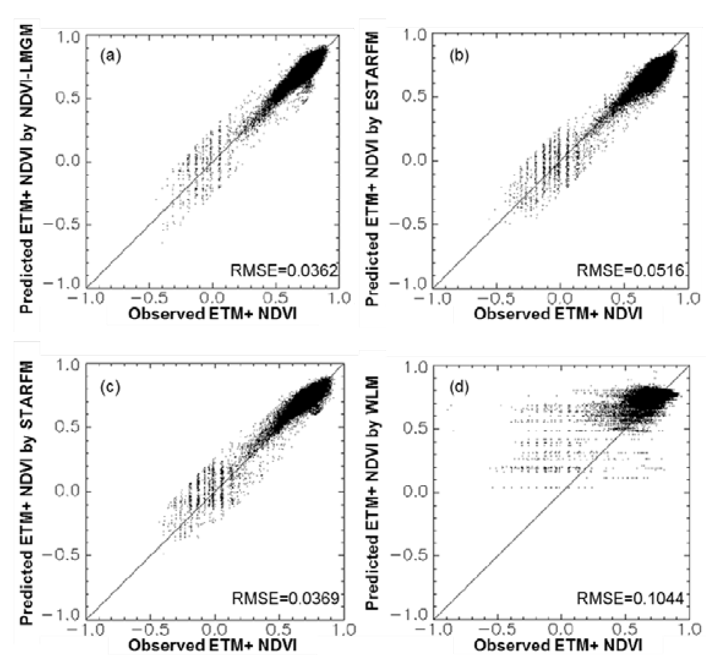
Experiments at three different sites have demonstrated that NDVI-LMGM performs better than the other three methods, STARFM, ESTARFM and WLM. Its superior performance may be attributed to the following advantages: (1) more reasonable assumptions; (2) better use of the information from base TM/ETM+ images; and (3) better selection of pixels with the same land cover type. These advantages will be explained in detail in the following sections.

First, the most important assumption of NDVI-LMGM is that neighboring pixels with the same land cover exhibit the same linear change (i.e., growth rate) during a short period. NDVI-LMGM has more practical and reasonable assumptions compared to the other methods. Generally, the growth of vegetation can be assumed to be under the influence of two groups of controlling factors. The first are biotic factors (e.g., vegetation type), which are not highly dependent on their geo-location. The second are the environmental factors, such as soil conditions, temperature, precipitation, etc., which have a strong dependence on geo-location. NDVI is representative of vegetation greenness and vigor, so it is reasonable to consider NDVI as a function of these two groups of controlling factors. In the same way, the change pattern of NDVI (growth rate) is also determined by both biotic factors and environmental factors; however, environmental factors play a more significant role than biotic factors, because the variations in environmental factors over time are more considerable than that of the biotic factors alone. Consequently, NDVI change within the same land cover over a small area can be assumed to be similar, because (1) the same land cover type in a small area has similar biotic factors; and (2) environmental factors have less variation in a small area according to the Tobler’s First Law of Geography [38]. STARFM assumes that a MODIS pixel and all Landsat pixels within that MODIS pixel share similar change patterns, which ignores the variation in change pattern among land cover types [10]. This unreasonable assumption decreases STARFM’s performance in heterogeneous landscapes [13]. For ESTARFM, it estimates the linear change rate between two Landsat observation dates and applies it to estimate the reflectance changes between the observation dates and any prediction dates during two observation dates [13]. However, the assumption of ESTARFM is invalid in some real situations, especially for areas with frequent cloud contamination or temporally heterogeneous landscapes, in which rapid changes can occur in a short time. For WLM, the basic assumption is that each land cover class has the same NDVI value regardless of the differences in biotic and environmental conditions [22]. This assumption cannot hold true in reality due to the diversity of environmental conditions and biotic characteristics, which can result in significant variation of NDVI values within the same land cover class in a larger area, also referred to as spectral variability when used in spectral mixture analysis [23].

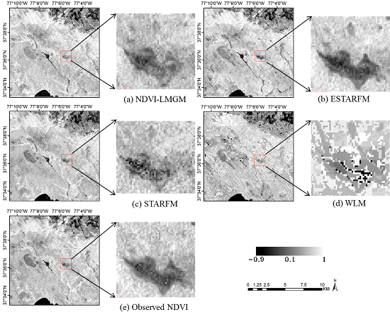
Second, NDVI-LMGM makes better use of the spatial information from Landsat observations. In NDVI-LMGM, the original Landsat-scale NDVI value is used (i.e., the Landsat observation) as the basic value to which the predicted Landsat-scale NDVI changes are added. This method retains spatial details very well since the base Landsat image preserves more spatial details. 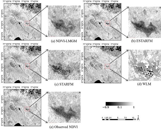On the other hand, WLM only uses the Landsat images to obtain constant weights for the linear system, which ignores the within-class variations and results in a strong patchy effect (Figure 9). In addition, STARFM and ESTARFM both employ a weighted average procedure for predictions from all neighboring similar pixels. Although it would improve the prediction results to some extent, it also might produce smoother prediction results while some spatial details could be lost.

Third, an important step for all the methods is to determine the pixels that share the same change patterns, also referred to as similar pixels or pixels with same land cover. NDVI-LMGM employs ISODATA to classify all available Landsat images to obtain the land cover map. As we know, multi-temporal images can improve the land cover classification because temporal information is an important supplement to spectral information, which helps differentiate various land covers. Therefore, it is expected that NDVI-LMGM can accurately select pixels of similar land cover. Unlike NDVI-LMGM, WLM uses existing fine-resolution land cover maps to select pixels of similar land cover, which has two limitations (1) high-quality land cover maps are often unavailable; and (2) temporal mismatching between the land cover map and prediction dates might introduce errors in the downscaling process because land cover often changes over time. Both STARFM and ESTARFM use one or two base images to select similar pixels based on a threshold of spectral distance. This procedure may introduce significant errors in similar pixel selection when the base images are further away from the prediction date. In addition, the determination of the threshold is very empirical, which might affect the robustness of STARFM and ESTARFM.

Along with the above advantages, which lead to a more accurate prediction, NDVI-LMGM is more efficient in computational time than the three other methods, especially when compared to indirect methods, such as ESTARFM. As mentioned above, all current methods (i.e., STARFM, ESTARFM and WLM) require a procedure for identifying similar pixels within each target area, which is very time-consuming. Instead, NDVI-LMGM directly employs neighboring MODIS pixels and the land cover result to build a linear model system. The high efficiency of NDVI-LMGM makes it appropriate for large-scale applications.

4.2. Influence of Parameters in NDVI-LMGM

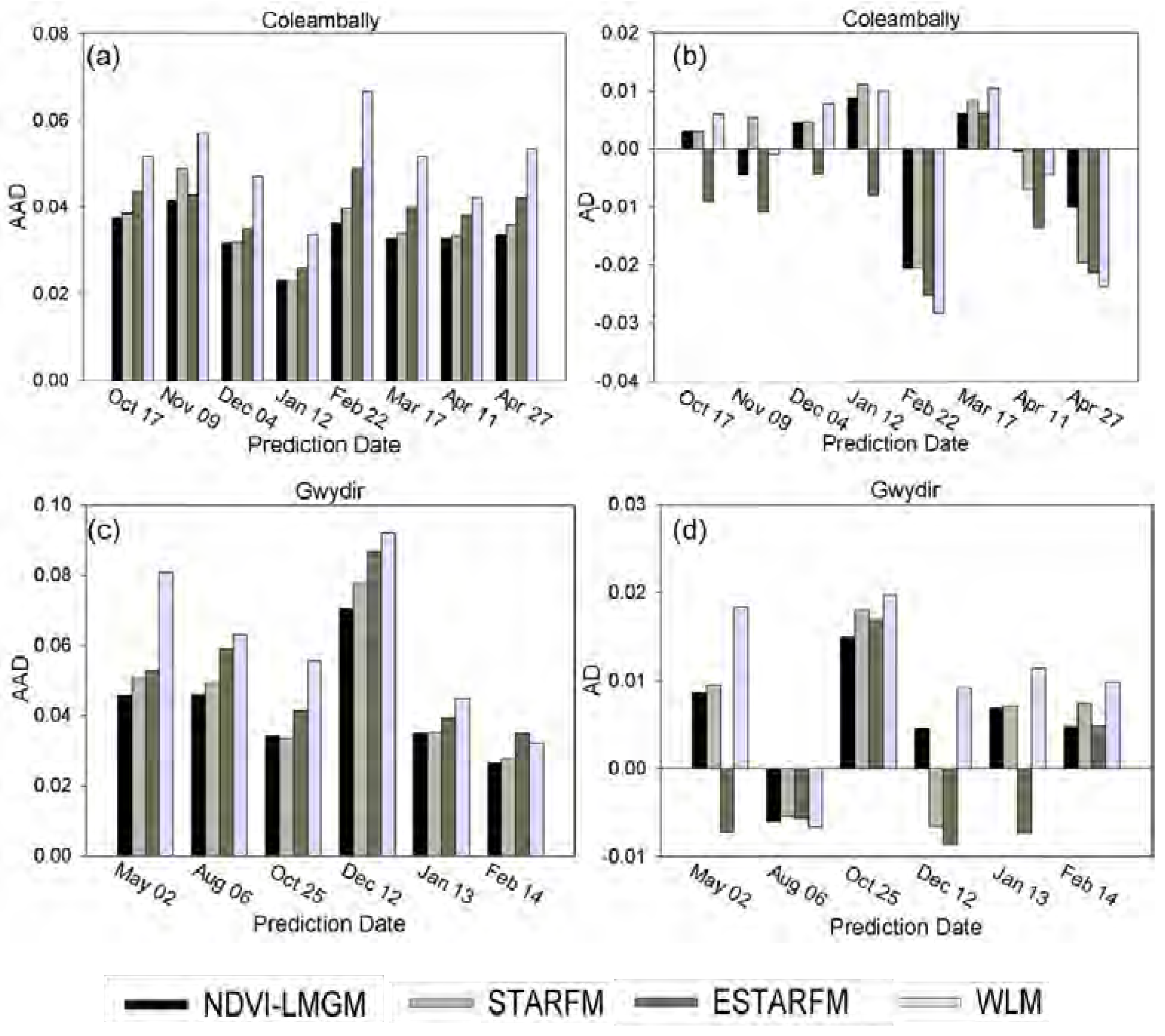
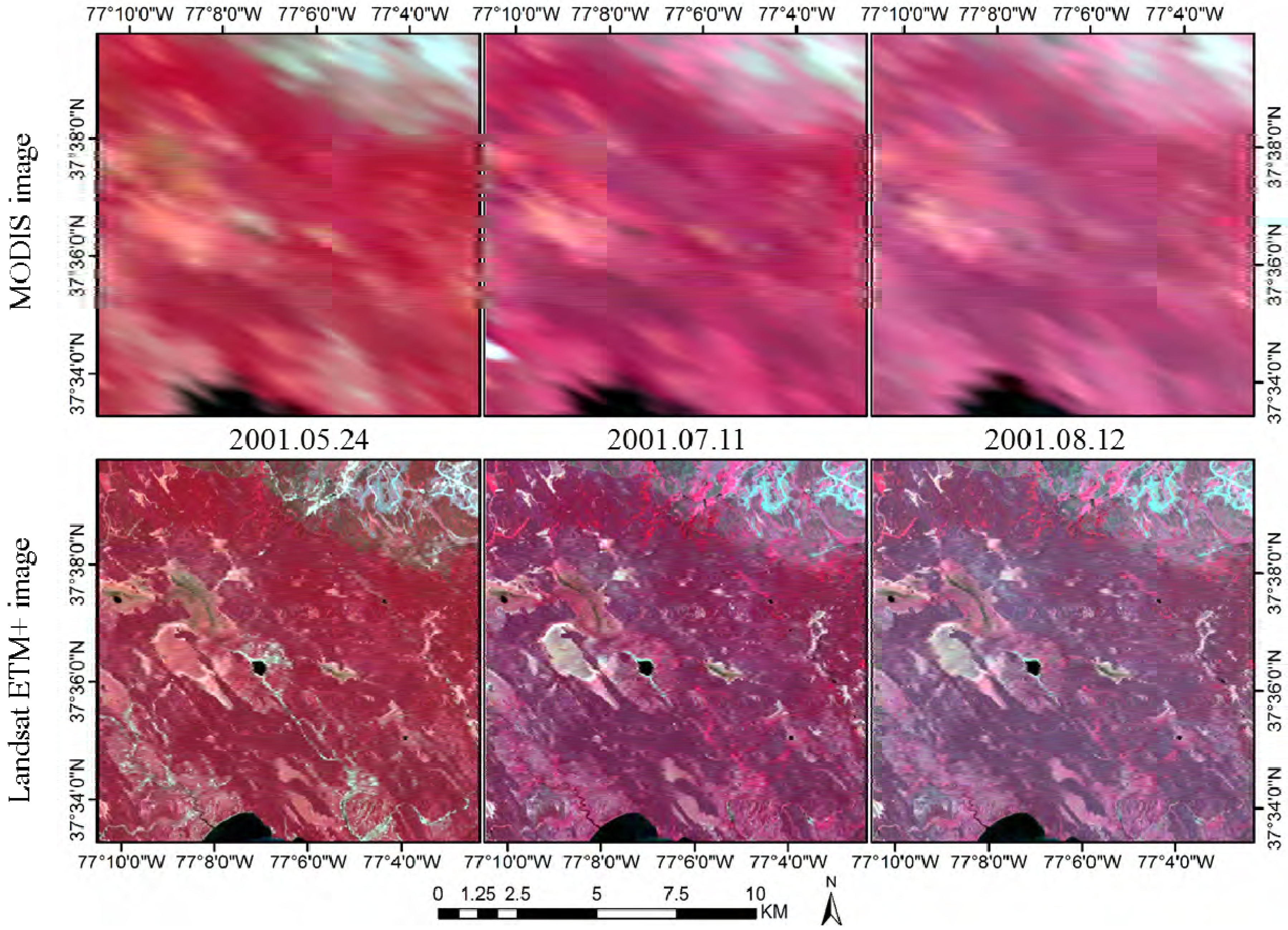
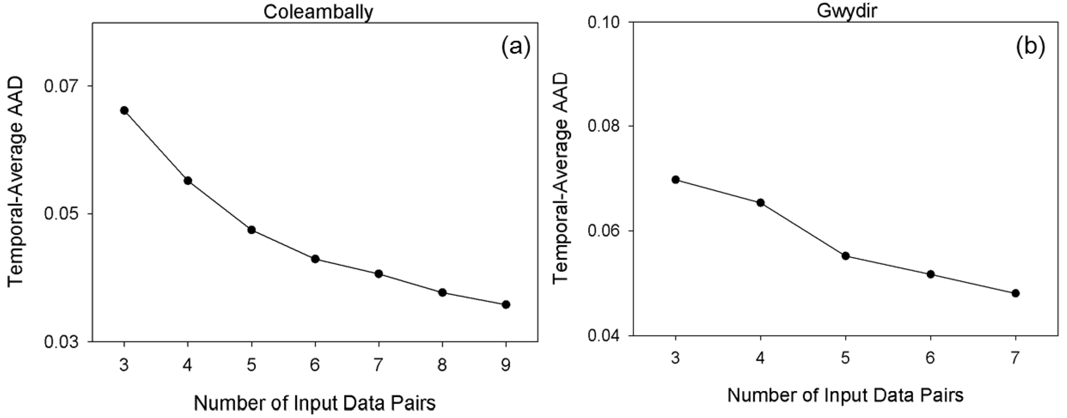
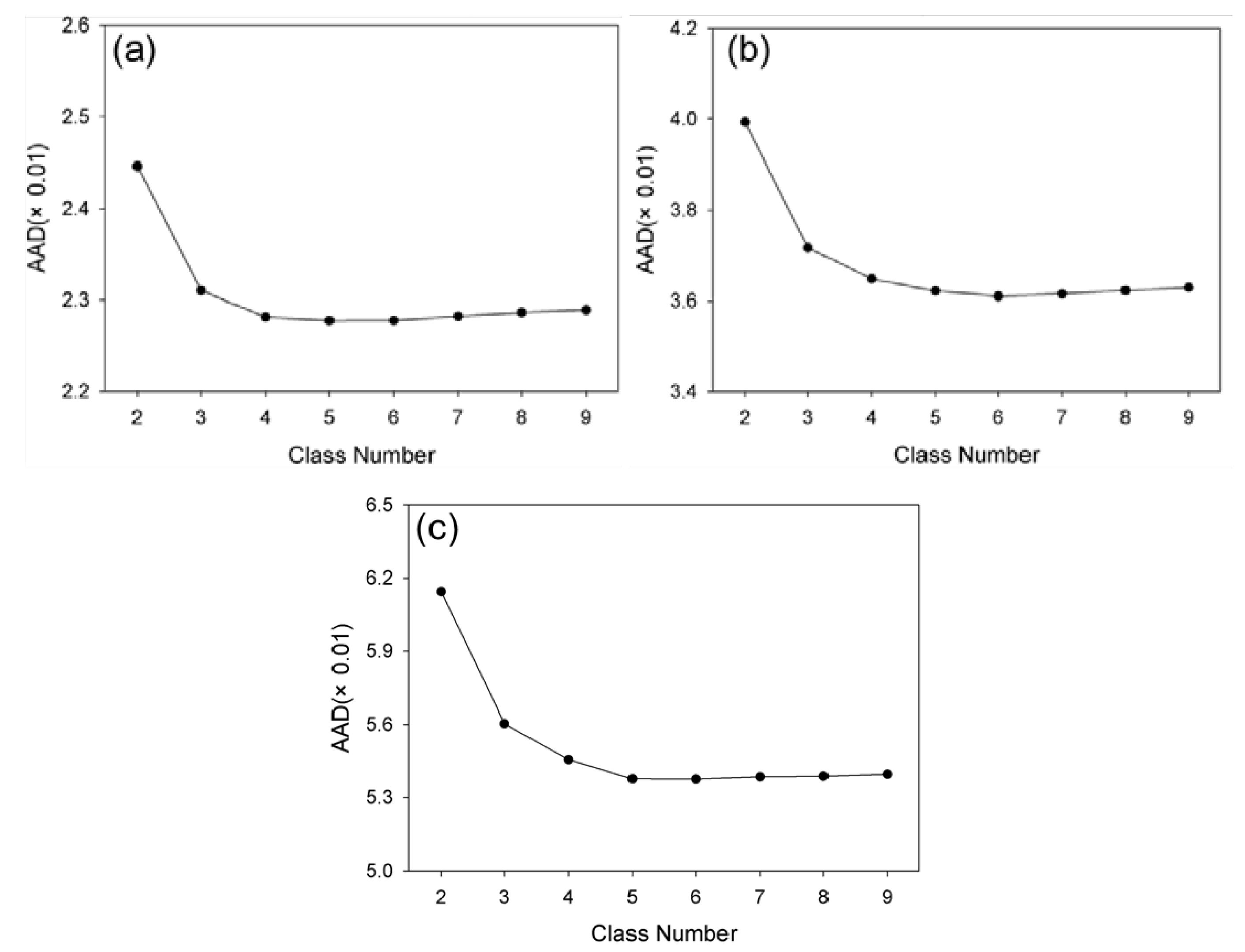
As described, the class number in unsupervised classification is empirically determined by users. Therefore, it is necessary to investigate the influence of the class numbers for prediction accuracy. Accordingly, experiments were conducted in the forest site and two Australian sites using various class numbers in unsupervised classification (i.e., two-nine classes in this study). For the forest site, 11 July 2001 was used as the prediction date and the other two pairs were used as input. For Coleambally, 12 February 2002 was selected as the prediction date and image pairs on 11 January and 21 February were used as input. Lastly, for Gwydir, 2 May 2004 was the prediction date and image pairs on 16 April and 5 July were set as inputs.

Figure 14. The prediction error (AAD) vs. class number for three study sites, (a) the forest site (prediction date: 11 July 2001); (b) Coleambally site (prediction date: 12 February 2002); and (c) Gwydir site (prediction date: 2 May 2004).

Figure 14. The prediction error (AAD) vs. class number for three study sites, (a) the forest site (prediction date: 11 July 2001); (b) Coleambally site (prediction date: 12 February 2002); and (c) Gwydir site (prediction date: 2 May 2004).

Figure 15 illustrates the prediction error (AAD) against the numbers of classes in the three test sites. Although AAD values vary according to the number of classes, these variation ranges are relatively small at 0.0017, 0.0038 and 0.0076, respectively, indicating that NDVI-LMGM is not highly sensitive to the number of classes. Moreover, there was a general trend among the three sites in which the AAD decreased at first, and then became stable followed by a slight increase as the class number steadily increased (Figure 14). Although the trends are similar, the change points from a decreasing to an increasing curve, representing the optimal class number, are different. Specifically, the class number corresponding to the change point for the forest site was four, while it was six and five for the Coleambally and Gwydir, respectively. It is obvious that the optimal class number in a relatively homogenous site, such as the forest site, was lower than those in spatially heterogeneous sites, such as the two Australian sites. This finding substantiates the guideline of ISODATA classification in NDVI-LMGM that the more complex the landscape in the study area, the more class numbers should be established. It also indicates that the class number of four, five or six could be recommended for applications according to the complexity of landscapes, which may ensure a satisfactory prediction result of NDVI-LMGM.

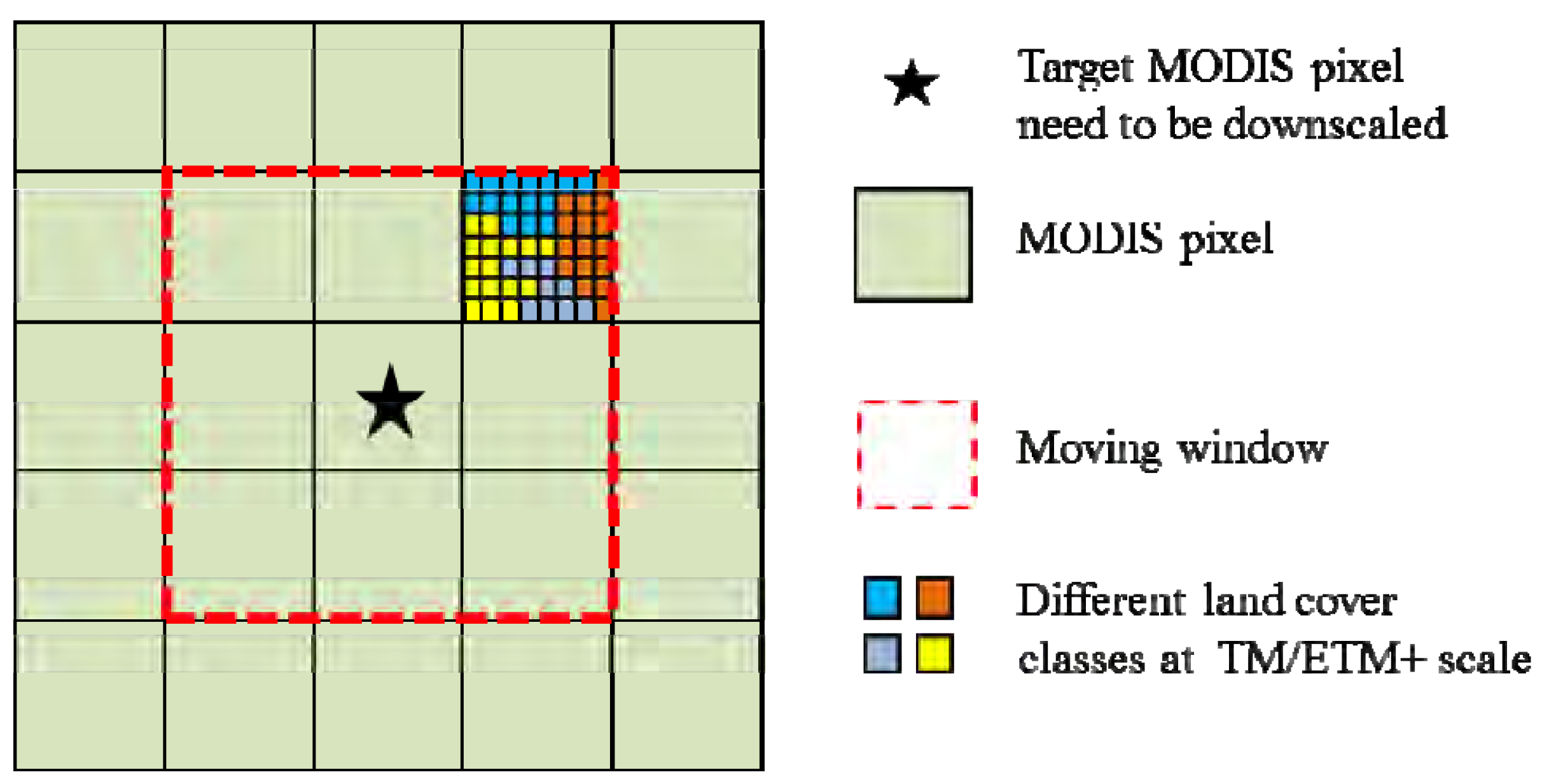
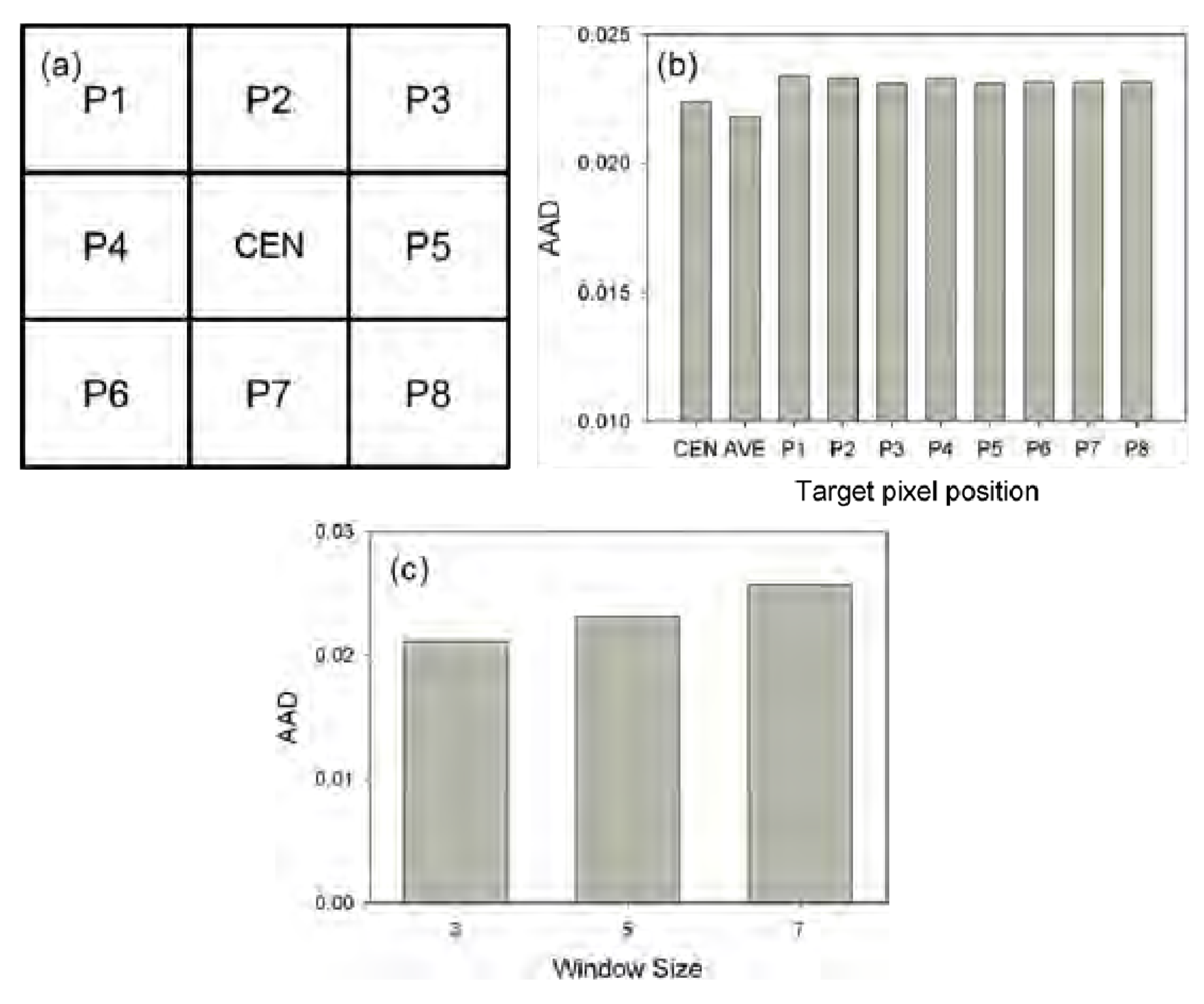
The growth rate from t₁ to t₂ at TM scale is the most important parameter required to be estimated in NDVI-LMGM. Specifically, spatially neighboring MODIS pixels have been employed to solve a linear model system (Equation (4)), resulting in a situation in which each MODIS pixel is used several times and the same number of growth rates for each MODIS pixel can be obtained when it is located in varying positions of a moving window (e.g., nine times for each MODIS pixel when the moving window size is set as 3 × 3). However, in NDVI-LMGM, only the growth rate can be estimated when the MODIS pixel located in the center of the window (Figure 15a) is used for prediction (Equation (1)). How does the performance change if the growth rate is estimated when a given MODIS pixel is at other positions within a moving window or the average of all estimated growth rates is used? To answer this question, an experiment was conducted in the forest site using the same data and parameter settings as those shown in Figure 8. As Figure 15b shows, the AAD values for using the growth rate estimated when the MODIS pixel was located in the center of the window or when the average of all estimated growth rates was used, both of them were lower than those using the growth rate estimated when a given MODIS pixel was at any other position within the moving window. Accordingly, considering the simplification of NDVI-LMGM, the growth rate estimated from the center of the window was finally adopted. In addition, the moving window size in NDVI-LMGM was also investigated in the forest study site. Figure 15c exhibits the AAD variation when three different window sizes were used. It was evident that the larger window size, after satisfying Equation (6), could introduce more significant errors into the prediction results, mainly because the larger window size may challenge the assumption underlying our method that the same land cover type has a similar growth rate in a small area Therefore, using the moving window with a size of 3 × 3 is recommended if the number of land cover classes is set to less than nine.

Figure 15. (a) The MODIS pixels within a moving window used to solve a linear model system, CEN indicates the center of the moving window. (b) The performance comparison by using different growth rates estimated from different positions of a moving window. Here, AVE stands for averaged growth rate of all growth rates. (c) The AAD comparison using different window sizes.

Figure 15. (a) The MODIS pixels within a moving window used to solve a linear model system, CEN indicates the center of the moving window. (b) The performance comparison by using different growth rates estimated from different positions of a moving window. Here, AVE stands for averaged growth rate of all growth rates. (c) The AAD comparison using different window sizes.

4.3. The Limitations of NDVI-LMGM

In addition to the strengths mentioned, NDVI-LMGM also has some limitations that should be noted. First, as discussed in Section 4.2, the number of classes will affect its prediction performance. Also, the parameters of class number should be determined according to the complexity of the landscape in the study area. The presence of multi-temporal Landsat images would help to improve the classification and prediction results. However, we acknowledge here that using smaller numbers of classifications can create errors, which would also affect the NDVI prediction accuracy of our method even if the temporal TM/ETM+ images are used in classification. As an operational method, we must accept such imperfect results because obtaining a perfect classification by using any up-to-date classifier is currently unpractical. However, it is expected that any attempts to improve classification accuracy will benefit our method after it is integrated into our system.

The prediction results would be influenced by the composite process of the MODIS data. Walker et al. has analyzed how this process would affect the results of STARFM [14]. The study revealed that the composite product (including 8-day MOD09A1 and 16-day NBAR (MCD43A3)) could be problematic, especially for the regions that experience rapid vegetation changes. However, the use of composite datasets during the peak of the growing season has the advantage that vegetation states is not likely to change appreciably during an 8- or 16-day period. Thus, for the region with rapid vegetation changes, the daily MODIS product (i.e., MOD09GA) is a better option for use as input. Moreover, the acquisition date of the input data also has an inevitable influence on the prediction performance (Section 3.3), which is similar to other existing methods [10,13,14].

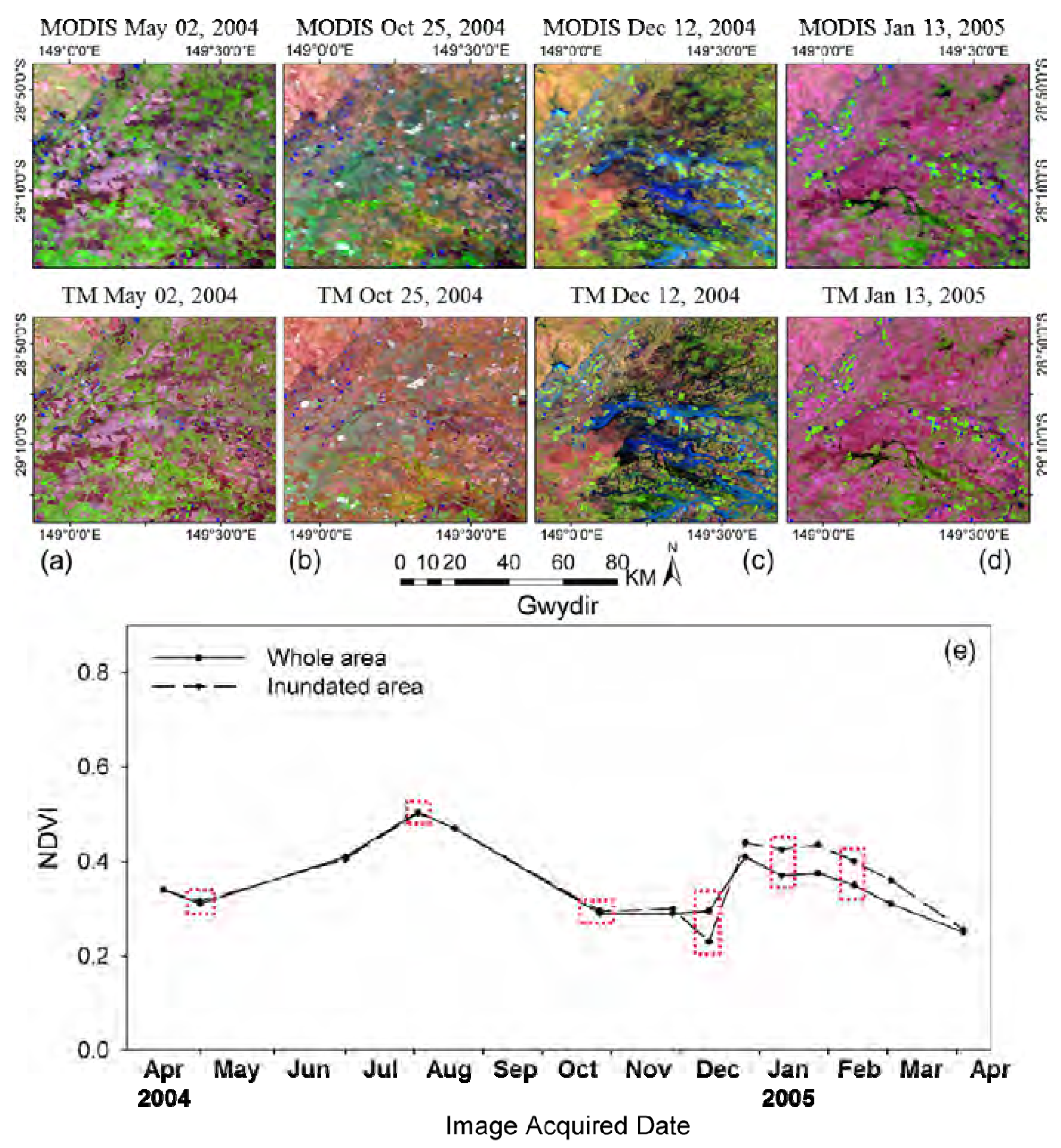
Additionally, it should be noted that small-scale land cover changes occurred between the observation date and prediction date might impact on the prediction, especially when only single observed image are used for clustering. These small-scale changes may not been detected in the classification map, thus leading to large errors for these regions. This drawback could be found in tests over Gwydir when the flood suddenly occurred to that region (Section 3.3). Fortunately, if there are multi-temporal high spatial resolution image that can be used for clustering, these land cover changes could be captured based on their different temporal change information from other land cover types.

5. Conclusion

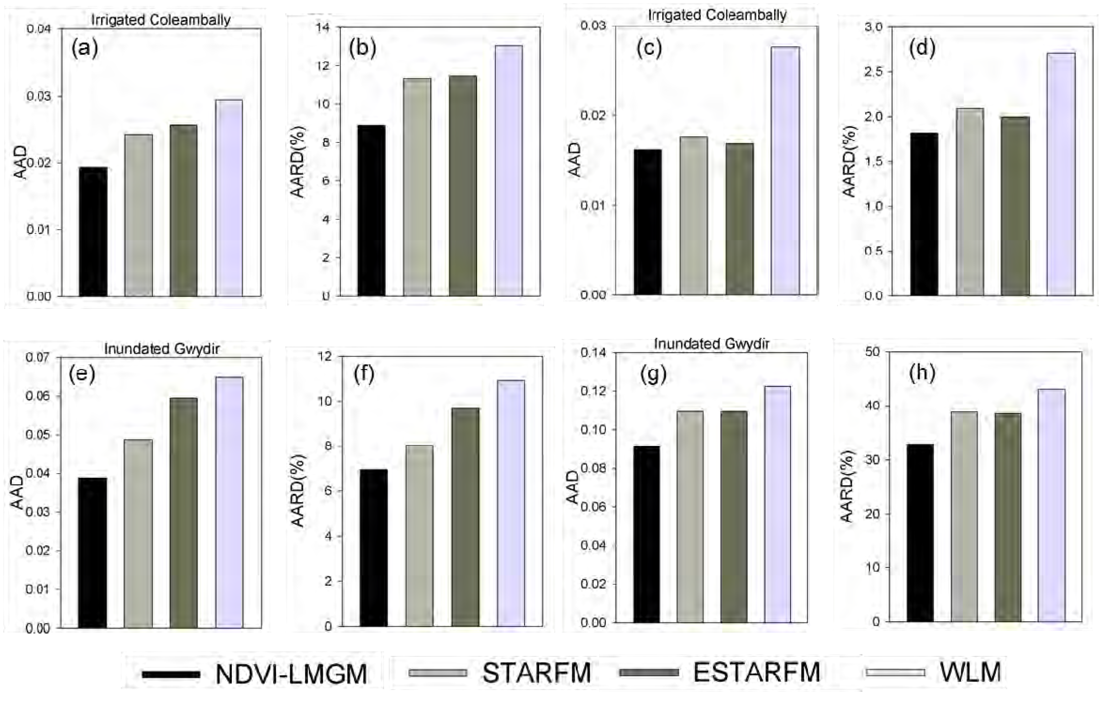
This study proposed a new method, NDVI-LMGM, to produce high spatial resolution NDVI time-series data by using MODIS NDVI time-series data and Landsat images. As demonstrated by experiments at three different sites with contrasting spatial and temporal heterogeneity, we found that NDVI-LMGM could produce high spatial resolution NDVI time-series dataset with smaller errors (with the average absolute difference less than 0.08 and average absolute relative difference less than 9% for three experiments) and less bias compared to STARFM, ESTARFM and WLM.

NDVI-LMGM combines the NDVI Linear Mixing model with the NDVI Linear Growth model, with which the NDVI prediction problem can be transformed into solving a linear system. Since there are several growth rates for different land cover classes at the Landsat scale, which require estimation in the linear system, the extra information from the spatially neighboring MODIS pixels was employed based on the assumption that spatially neighboring pixels with the same land cover type in a small area have similar growth rates. Compared with the assumptions needed for STARFM, ESTARFM and WLM, the NDVI-LMGM’s assumption is easier to satisfy and is more reasonable. In order to obtain more accurate land cover classification results, NDVI-LMGM employs all available multi-temporal Landsat images for ISODATA classification. Although the performance of NDVI-LMGM would be affected by various classification results and input Landsat images, it is expected that the new method can provide an alternative for directly downscaling NDVI products with higher accuracy and less computational cost. In addition, such downscaled NDVI products will benefit studies of ecosystem dynamics as one crucial aspect of understanding global climate change. In future studies, more efforts should be spent to reduce the influence of land cover classification and small-scale land cover type changes to the prediction results.

References

1. Rouse, J., Jr.; Haas, R.; Schell, J.; Deering, D. Monitoring vegetation systems in the Great Plains with ERTS. In Proceedings of Third ERTS Symposium, Washington, DC, USA, 10–14 December 1973; pp. 309–317.
2. Tucker, C.J. Red and photographic infrared linear combinations for monitoring vegetation. Remote Sens. Environ. 1979, 8, 127–150. [Google Scholar] [CrossRef]
3. Huete, A.; Didan, K.; Miura, T.; Rodriguez, E.P.; Gao, X.; Ferreira, L.G. Overview of the radiometric and biophysical performance of the MODIS vegetation indices. Remote Sens. Environ. 2002, 83, 195–213. [Google Scholar] [CrossRef]
4. Pettorelli, N.; Vik, J.O.; Mysterud, A.; Gaillard, J.M.; Tucker, C.J.; Stenseth, N.C. Using the satellite-derived NDVI to assess ecological responses to environmental change. Trends Ecol. Evol. 2005, 20, 503–510. [Google Scholar] [CrossRef] [PubMed]
5. Shabanov, N.V.; Zhou, L.M.; Knyazikhin, Y.; Myneni, R.B.; Tucker, C.J. Analysis of interannual changes in northern vegetation activity observed in AVHRR data from 1981 to 1994. IEEE Trans. Geosci. Remote Sens. 2002, 40, 115–130. [Google Scholar] [CrossRef]
6. Lenney, M.P.; Woodcock, C.E.; Collins, J.B.; Hamdi, H. The status of agricultural lands in Egypt: The use of multitemporal NDVI features derived from Landsat TM. Remote Sens. Environ. 1996, 56, 8–20. [Google Scholar] [CrossRef]
7. Seto, K.C.; Fleishman, E.; Fay, J.P.; Betrus, C.J. Linking spatial patterns of bird and butterfly species richness with Landsat TM derived NDVI. Int. J. Remote Sens. 2004, 25, 4309–4324. [Google Scholar] [CrossRef]
8. Gonzalez-Sanpedro, M.C.; Le Toan, T.; Moreno, J.; Kergoat, L.; Rubio, E. Seasonal variations of leaf area index of agricultural fields retrieved from Landsat data. Remote Sens. Environ. 2008, 112, 810–824. [Google Scholar] [CrossRef]
9. Ranson, K.J.; Kovacs, K.; Sun, G.; Kharuk, V.I. Disturbance recognition in the boreal forest using radar and Landsat-7. Can. J. Remote Sens. 2003, 29, 271–285. [Google Scholar] [CrossRef]
10. Gao, F.; Masek, J.; Schwaller, M.; Hall, F. On the blending of the Landsat and MODIS surface reflectance: Predicting daily Landsat surface reflectance. IEEE Trans. Geosci. Remote Sens. 2006, 44, 2207–2218. [Google Scholar]
11. Hilker, T.; Wulder, M.A.; Coops, N.C.; Linke, J.; McDermid, G.; Masek, J.G.; Gao, F.; White, J.C. A new data fusion model for high spatial- and temporal-resolution mapping of forest disturbance based on Landsat and MODIS. Remote Sens. Environ. 2009, 113, 1613–1627. [Google Scholar] [CrossRef]
12. Hilker, T.; Wulder, M.A.; Coops, N.C.; Seitz, N.; White, J.C.; Gao, F.; Masek, J.G.; Stenhouse, G. Generation of dense time series synthetic landsat data through data blending with MODIS using a spatial and temporal adaptive reflectance fusion model. Remote Sens. Environ. 2009, 113, 1988–1999. [Google Scholar] [CrossRef]
13. Zhu, X.L.; Chen, J.; Gao, F.; Chen, X.H.; Masek, J.G. An enhanced spatial and temporal adaptive reflectance fusion model for complex heterogeneous regions. Remote Sens. Environ. 2010, 114, 2610–2623. [Google Scholar] [CrossRef]
14. Walker, J.J.; de Beurs, K.M.; Wynne, R.H.; Gao, F. Evaluation of Landsat and MODIS data fusion products for analysis of dryland forest phenology. Remote Sens. Environ. 2012, 117, 381–393. [Google Scholar] [CrossRef]
15. Jarihani, A.; McVicar, T.; van Niel, T.; Emelyanova, I.; Callow, J.; Johansen, K. Blending Landsat and MODIS data to generate multispectral indices: A comparison of “index-then-blend” and “blend-then-index” approaches. Remote Sens. 2014, 6, 9213–9238. [Google Scholar] [CrossRef] [Green Version]
16. Roy, D.P.; Ju, J.; Lewis, P.; Schaaf, C.; Gao, F.; Hansen, M.; Lindquist, E. Multi-temporal MODIS-Landsat data fusion for relative radiometric normalization, gap filling, and prediction of Landsat data. Remote Sens. Environ. 2008, 112, 3112–3130. [Google Scholar] [CrossRef]
17. Amoros-Lopez, J.; Gomez-Chova, L.; Alonso, L.; Guanter, L.; Zurita-Milla, R.; Moreno, J.; Camps-Valls, G. Multitemporal fusion of Landsat/TM and ENVISAT/MERIS for crop monitoring. Int. J. Appl. Earth Obs. Geoinf. 2013, 23, 132–141. [Google Scholar] [CrossRef]
18. Wu, M.; Niu, Z.; Wang, C.; Wu, C.; Wang, L. Use of MODIS and Landsat time series data to generate high-resolution temporal synthetic Landsat data using a spatial and temporal reflectance fusion model. J. Appl. Remote Sens. 2012, 6, 063507. [Google Scholar]
19. Zhukov, B.; Oertel, D.; Lanzl, F.; Reinhackel, G. Unmixing-based multisensor multiresolution image fusion. IEEE Trans. Geosci. Remote Sens. 1999, 37, 1212–1226. [Google Scholar] [CrossRef]
20. Settle, J.J.; Drake, N.A. Linear mixing and the estimation of ground cover proportions. Int. J. Remote Sens. 1993, 14, 1159–1177. [Google Scholar] [CrossRef]
21. Kerdiles, H.; Grondona, M.O. NOAA-AVHRR NDVI decomposition and subpixel classification using linear mixing in the Argentinean Pampa. Int. J. Remote Sens. 1995, 16, 1303–1325. [Google Scholar] [CrossRef]
22. Busetto, L.; Meroni, M.; Colombo, R. Combining medium and coarse spatial resolution satellite data to improve the estimation of sub-pixel NDVI time series. Remote Sens. Environ. 2008, 112, 118–131. [Google Scholar] [CrossRef]
23. Somers, B.; Asner, G.P.; Tits, L.; Coppin, P. Endmember variability in spectral mixture analysis: A review. Remote Sens. Environ. 2011, 115, 1603–1616. [Google Scholar] [CrossRef]
24. Meng, J.H.; Du, X.; Wu, B.F. Generation of high spatial and temporal resolution NDVI and its application in crop biomass estimation. Int. J. Digit. Earth 2013, 6, 203–218. [Google Scholar] [CrossRef]
25. Adams, J.B.; Smith, M.O.; Johnson, P.E. Spectral mixture modeling—A new analysis of rock and soil types at the Viking Lander 1 site. J. Geophys. Res.: Atmos. 1986, 91, 8098–8112. [Google Scholar] [CrossRef]
26. Aman, A.; Randriamanantena, H.P.; Podaire, A.; Frouin, R. Upscale integration of normalized difference vegetation index: The problem of spatial heterogeneity. IEEE Trans. Geosci. Remote Sens. 1992, 30, 326–338. [Google Scholar] [CrossRef]
27. Ju, J.C.; Roy, D.P. The availability of cloud-free Landsat ETM plus data over the conterminous United States and globally. Remote Sens. Environ. 2008, 112, 1196–1211. [Google Scholar] [CrossRef]
28. Zhu, X.L.; Gao, F.; Liu, D.S.; Chen, J. A modified neighborhood similar pixel interpolator approach for removing thick clouds in landsat images. IEEE Trans. Geosci. Remote Sens. 2012, 9, 521–525. [Google Scholar] [CrossRef]
29. Gao, F.; Masek, J.; Wolfe, R.E. Automated registration and orthorectification package for landsat and landsat-like data processing. J. Appl. Remote Sens. 2009, 3. [Google Scholar] [CrossRef]
30. Masek, J.G.; Collatz, G.J. Estimating forest carbon fluxes in a disturbed southeastern landscape: Integration of remote sensing, forest inventory, and biogeochemical modeling. J. Geophys. Res.: Biogeosci. 2006, 111. [Google Scholar] [CrossRef]
31. Moody, E.G.; King, M.D.; Platnick, S.; Schaaf, C.B.; Gao, F. Spatially complete global spectral surface albedos: Value-added datasets derived from terra MODIS land products. IEEE Trans. Geosci. Remote Sens. 2005, 43, 144–158. [Google Scholar] [CrossRef]
32. Chen, J.; Jonsson, P.; Tamura, M.; Gu, Z.H.; Matsushita, B.; Eklundh, L. A simple method for reconstructing a high-quality NDVI time-series data set based on the Savitzky-Golay filter. Remote Sens. Environ. 2004, 91, 332–344. [Google Scholar] [CrossRef]
33. Huang, C.Q.; Townshend, J.R.G.; Liang, S.L.; Kalluri, S.N.V.; DeFries, R.S. Impact of sensor’s point spread function on land cover characterization: Assessment and deconvolution. Remote Sens. Environ. 2002, 80, 203–212. [Google Scholar] [CrossRef]
34. Townshend, J.R.G.; Huang, C.; Kalluri, S.N.V.; Defries, R.S.; Liang, S.; Yang, K. Beware of per-pixel characterization of land cover. Int. J. Remote Sens. 2000, 21, 839–843. [Google Scholar] [CrossRef]
35. Guerschman, J.P.; Paruelo, J.M.; Di Bella, C.; Giallorenzi, M.C.; Pacin, F. Land cover classification in the argentine pampas using multi-temporal Landsat TM data. Int. J. Remote Sens. 2003, 24, 3381–3402. [Google Scholar] [CrossRef]
36. Yuan, F.; Sawaya, K.E.; Loeffelholz, B.C.; Bauer, M.E. Land cover classification and change analysis of the Twin Cities (Minnesota) Metropolitan Area by multitemporal Landsat remote sensing. Remote Sens. Environ. 2005, 98, 317–328. [Google Scholar] [CrossRef]
37. Emelyanova, I.V.; McVicar, T.R.; Van Niel, T.G.; Li, L.T.; van Dijk, A.I.J.M. Assessing the accuracy of blending Landsat-MODIS surface reflectances in two landscapes with contrasting spatial and temporal dynamics: A framework for algorithm selection. Remote Sens. Environ. 2013, 133, 193–209. [Google Scholar] [CrossRef]
38. Tobler, W.R. A computer movie simulating urban growth in Detroit region. Econ. Geogr. 1970, 46, 234–240. [Google Scholar] [CrossRef]